Test of the Schrödinger functional with chiral fermions in the Gross-Neveu model

Abstract:

The recently proposed construction of chiral fermions on lattices with boundaries is tested in an interacting theory up to first order of perturbation theory. We confirm that, in the bulk of the lattice, the chiral Ward identities take their continuum value up to cutoff effects without any tuning. Universal quantities are defined that have an expansion in the renormalised couplings with coefficients that are functions of the physical size and the periodicity in the spatial direction. These coefficient functions have to be identical for different discretisations. We find agreement with the standard Wilson fermions. The computation is done in the asymptotically free Gross-Neveu model with continuous chiral symmetry.

1 Introduction

We present a 1-loop perturbative calculation that confirms the favourable properties of chiral fermions on a lattice with boundaries [1]. The calculation is performed in the chiral Gross-Neveu model [2]. Before I go into the details and results of the calculation let me briefly introduce field theories on lattices with boundaries.

In the Schrödinger functional (SF) of a quantum field theory the fields are defined on a $d+1$ dimensional cylinder. The fields are subject to Dirichlet boundary conditions in the time direction ($P_{\pm}=\tfrac{1}{2}(1\pm\gamma_{0})$)

$$P_{+}\psi(x)=0\,,\quad\overline{\psi}(x)P_{-}=0\quad\text{at}\quad x_{0}=0\,,$$ (1)

$$P_{-}\psi(x)=0\,,\quad\overline{\psi}(x)P_{+}=0\quad\text{at}\quad x_{0}=T$$ (2)

and periodic boundary conditions in the space directions

$$\psi(x+L\hat{k})=\mathrm{e}^{i\theta}\psi(x)\,,\quad\theta\in[0,2\pi)\,,\quad k=1,\dots d\,.$$ (3)

Discretising such a theory on a space-time lattice with boundaries has advantages. If the temporal extension is a multiple of the spatial extension, say $T=2L$, the inverse of the spatial extension $1/L$ provides an infrared cutoff and is the natural energy scale in the massless theory. In fact this has enabled a fully non-perturbative determination of the scale dependence of the fundamental parameters of $N_{\mathrm{f}}=2$ QCD, see [3] and references therein.

However, naively one would expect that theories become more complicated on lattices with boundaries. First of all the distinction between different classes of boundary conditions, for example Dirichlet and Neuberger boundary conditions, really only makes sense for smooth fields, which we do not have on the lattice. The boundary conditions therefore must be encoded in the lattice action and will arise dynamically in the continuum limit. In general this might involve the necessity to fine-tune some parameter in the action. Secondly the boundaries might cause additional divergences and thus lead to additional counter-terms. Both of these issues have been addressed for QCD in [4] with the result that there is no need for fine-tuning and that one just has to add a renormalisation factor for the boundary fields.

The fact that the SF boundary conditions arise naturally (without fine-tuning) in the continuum limit has been understood on the basis of dimensional counting and boundary critical phenomena, see [1] and references therein. The SF boundary conditions are part of the definition of the continuum limit. Together with the symmetry properties and the dimensionality of the system they form a SF universality class: any local discretisation has this continuum limit.

Exactly this observation led the author of [1] to a formulation of the lattice SF of QCD with chiral fermions. In the continuum the SF boundary conditions break chiral symmetry. Therefore lattice fermions that fulfil the Ginsparg-Wilson relation [6] on the whole lattice (with boundaries) can not have the right continuum limit. The minimal modification to the Ginsparg-Wilson relation that breaks the lattice chiral symmetry at the boundary would be a term $\Delta_{B}$ that is supported at the boundary with exponentially decaying tails

$$\gamma_{5}\,D+D\,\gamma_{5}=a\,D\gamma_{5}D+\Delta_{B}\,.$$ (4)

Given a local solution to this equation chiral Ward identities are expected to take their continuum form far away from the boundaries.

As mentioned above, in principle there are many possible local lattice formulations that have the same continuum limit. In [1] the author gives one solution to the modified Ginsparg-Wilson relation, a modified Neuberger-Dirac operator

$$D=\tfrac{1}{\bar{a}}\left\{1-\tfrac{1}{2}(U+\gamma_{5}U^{\dagger}\gamma_{5})\right\}\,,$$ (5)

$$U=A\,(A^{\dagger}A+caP)^{-1/2}\,,\quad\bar{a}=\frac{a}{1+s}\,,\quad A=1+s-aD_{\text{W}}\,,$$ (6)

where $D_{\text{W}}$ is the massless Wilson-Dirac operator in the presence of the boundaries as introduced in [4], i.e. the standard infinite lattice Wilson-Dirac operator in the range $0<x_{0}<T$ and at all other times the target field $\chi=D_{W}\psi$ is set to zero. The projector $P$ is defined through

$$P\psi(x)=\frac{1}{a}\left\{\delta_{x_{0},a}P_{-}\psi(x)\big{|}_{x_{0}=a}+\delta_{x_{0},T-a}P_{+}\psi(x)\big{|}_{x_{0}=T-a}\right\}\,,$$ (7)

and the parameters $c$ and $s$ must be chosen such as to ensure locality (see next section). The operator (5) solves (4) if the lattice spacing $a$ is replaced by the rescaled value $\bar{a}$. For all unexplained notation we refer the reader to [7].

2 Free fermions

For Wilson fermions the free propagator in presence of the boundaries can be calculated explicitly and is given in [8]. In the case of chiral fermions we do not even have an analytic expression for the Dirac operator. To obtain the free propagator in closed form like in the Wilson case might be possible but is much more difficult. Nevertheless, the operator under the square root in (5) can be worked out in the time-momentum representation.

Taking into account the definition of $D_{\text{W}}$ in the presence of the boundaries given above, the operator under the square root explicitly reads

$$A^{\dagger}A+caP=(1+s)^{2}+sa^{2}\sum_{\mu}{\partial^{\ast}}_{\mspace{-11.0mu}\mu}\partial_{\mu}+\tfrac{1}{2}a^{4}\sum_{\mu<\nu}{\partial^{\ast}}_{\mspace{-11.0mu}\mu}\partial_{\mu}{\partial^{\ast}}_{\mspace{-11.0mu}\nu}\partial_{\nu}+(c-1)aP\,,$$ (8)

with forward $\partial_{\mu}\psi(x)=\tfrac{1}{a}(\psi(x+a\hat{\mu})-\psi(x))$ and backward ${\partial^{\ast}}_{\mspace{-11.0mu}\mu}\psi(x)=\tfrac{1}{a}(\psi(x)-\psi(x-a\hat{\mu}))$ finite differences. It is Hermitian and therefore has real eigenvalues. Due to translation invariance in space the spatial eigenfunctions are plane waves with momentum values that are integer multiples of $2\pi/L$ in the range $-\pi/a<p_{k}\leq\pi/a$. For $c=1$ the operator (8) is diagonal in Dirac space, so its eigenvalues are $2^{(d+1)/2}$-fold degenerated. Its eigenfunctions (in space-time) are then given by

$$c=1:\quad v_{p_{0},\mathbf{{p}}}(x)=\mathrm{e}^{i\mathbf{{p}}\mathbf{{x}}}\,\sin(p_{0}x_{0})\,,\quad p_{0}=\frac{n\pi}{T}\,,\quad n=1,2,\dots,T/a-1\,.$$ (9)

For $c\neq 1$ the operator (8) is not diagonal in Dirac space. The eigenfunctions are still given in terms of $\sin$-functions

$$c\neq 1:\quad w_{p_{0},\mathbf{{p}}}(x)=\mathrm{e}^{i\mathbf{{p}}\mathbf{{x}}}\,\left\{P_{-}\sin\big{(}p_{0}x_{0}+b(p_{0})\big{)}+P_{+}\sin\big{(}p_{0}(T-x_{0})+b(p_{0})\big{)}\right\}\,,$$ (10)

where

$$b(p_{0})=-\arctan\left(\frac{\sin(ap_{0})}{\frac{q}{c-1}+\cos(ap_{0})}\right)\,,\quad q=\tfrac{a^{2}}{2}\hat{\mathbf{{p}}}^{2}-s\,,\quad\hat{p}_{\mu}=\tfrac{2}{a}\sin(ap_{\mu}/2)\,.$$ (11)

But the allowed values of $p_{0}$ are now given by the solutions of the transcendental equation

$$b(p_{0})=-p_{0}T\,.$$ (12)

In either case the eigenvalues are given by

$$\lambda_{p_{0},\mathbf{{p}}}=(1+s)^{2}-sa^{2}\hat{p}^{2}+\tfrac{a^{4}}{2}\sum_{\mu<\nu}\hat{p}_{\mu}^{2}\hat{p}_{\nu}^{2}\,.$$ (13)

Rewriting this as

$$\lambda_{p_{0},\mathbf{{p}}}=q\,a^{2}\hat{p}_{0}^{2}+(1+s)^{2}-sa^{2}\hat{\mathbf{{p}}}^{2}+\tfrac{a^{4}}{2}\sum_{k<l}\hat{p}_{k}^{2}\hat{p}_{l}^{2}\,,$$ (14)

one can easily show that the eigenvalues are bounded from below by $(1-|s|)^{2}$ for $|s|<1$ and $c\geq 1$. In particular, the constraint on $c$ ensures that the combination $q\,a^{2}\hat{p}_{0}^{2}$ is always positive.

Adopting the argument in ref. [9], using expansion in Legendre polynomials, we conclude that in the free theory the locality of the Dirac operator (5) is guaranteed for this range of parameter values.

The eigenfunctions (9) (or (10)) may be orthonormalised and used to write down an analytical expression for the kernel $D(x,y)$ of the Dirac operator. But the evaluation of $D(x,y)$ in this way would be very expensive, since it involves a sum over momenta $p_{0}$ which in turn are determined for each set of parameter values by the roots of a transcendental equation.

In our computation we used a different approach. First the operator (5) is half-Fourier-transformed to its time-momentum representation $\tilde{D}(x_{0},\mathbf{{p}})$. The square-root of the remaining $(d+1)(T-1)\times(d+1)(T-1)$-matrices (one for each value of $\mathbf{{p}}$) is computed with the min-max polynomial as explained in section 4 of [10]. For the final step, to obtain the propagator, we used the built-in inversion routine of MATLAB.

The so calculated modified Neuberger-Dirac operator has been inserted in the Ginsparg-Wilson relation to compute the difference $\Delta_{B}$ and to confirm, that it is in fact localised at the boundaries with exponentially decaying tails.

3 Chiral Gross-Neveu model

To test the operator (5) beyond free fermions we introduce a two-dimensional theory with four-fermion interactions. The euclidean continuum action of the chiral Gross-Neveu model can be given in the form

$$S^{c}_{\text{CGN}}=\int\mathrm{d}x^{2}\,\left\{\overline{\psi}\,\gamma_{\mu}\partial_{\mu}\,\psi-\tfrac{1}{2}g^{2}(O_{SS}-O_{PP})-\tfrac{1}{2}g_{V}^{2}O_{VV}\right\}\,,$$ (15)

$$O_{SS}=(\overline{\psi}\psi)^{2}\,,\quad O_{PP}=(\overline{\psi}\gamma_{5}\psi)^{2}\,,\quad O_{VV}=\sum_{\mu}(\overline{\psi}\gamma_{\mu}\psi)^{2}\,.$$ (16)

All Dirac and flavour indices are suppressed and contracted in a straightforward way. For $N$ flavours of fermions this action possesses an $U(N)$-flavour symmetry and an $U(1)$ continuous chiral symmetry. For a detailed derivation of the possible terms (in terms of renormalisability) see chapter 5 of ref. [7]. The terms in (15) are a full set of allowed terms that respect the above mentioned symmetries (plus euclidean symmetry). For $N\geq 2$ the model shares with QCD the property of an asymptotically free coupling (namely $g^{2}$).

Discretisation with Wilson fermions is straightforward. But since the Wilson term breaks chiral symmetry a mass term and an additional coupling have to be added

$$S_{\text{CGN,W}}=a^{2}\sum_{x}\,\big{\{}\overline{\psi}\,(D_{\text{W}}+m_{0})\,\psi-\tfrac{1}{2}g_{w}^{2}(O_{SS}-O_{PP})-\tfrac{1}{2}\delta_{P}^{2}O_{PP}-\tfrac{1}{2}g_{V,w}^{2}O_{VV}\big{\}}\,.$$ (17)

No additional coupling (or mass term) is necessary if one uses a Dirac operator that solves the Ginsparg-Wilson relation. Since such an operator comes with a lattice chiral symmetry [11], there are no other allowed dimension 2 operators. However, to make the action manifestly invariant under that symmetry, one has to add irrelevant dimension 3 operators via the substitution $\psi\to\hat{\psi}=(1-\tfrac{a}{2}D)\psi$ in the four-fermion interaction terms. The action then reads

$$S_{\text{CGN,GW}}=a^{2}\sum_{x}\,\left\{\overline{\psi}\,D\,\psi-\tfrac{1}{2}g_{gw}^{2}(\hat{O}_{SS}-\hat{O}_{PP})-\tfrac{1}{2}g_{V,gw}^{2}\hat{O}_{VV}\right\}\,.$$ (18)

Defining now the SF of the Gross-Neveu model is straightforward. Since it is asymptotically free (for $N\geq 2$, which we assume from now on), the scaling dimension of local fields is equal to their engineering dimension. Therefore the argument about the naturalness of the SF boundary conditions in QCD [1] holds also in the chiral Gross-Neveu model. And in [7] it is shown that just one additional renormalisation factor for the boundary fields has to be added.

4 Chiral Ward identity

The continuum chiral Ward identity

$$\bigl{\langle}\partial_{\mu}A_{\mu}(x)\,\mathcal{O}(y)\bigr{\rangle}=2m\bigl{\langle}P(x)\,\mathcal{O}(y)\bigr{\rangle}\,,\quad x\neq y$$ (19)

implies on the lattice for vanishing renormalised mass $m_{R}=0$

$$\langle\left(\mathcal{O}\right)_{\mathrm{R}}\,\widetilde{\partial}_{\mu}\left(A_{\mu}\right)_{\mathrm{R}}(x)\rangle=\mathrm{O}(a)\,.$$ (20)

This can be used to compute the critical value of the bare mass parameter $m_{0}$ and the chiral symmetry restoring value of the bare coupling $\delta_{P}$ in (17) to second order in perturbation theory (PT) [7].

As indicated in (20) there are chiral symmetry breaking effects that are lattice artifacts. In this section we compute these effects for Wilson fermions and the proposed chiral fermions. To this end correlation functions that match the operators in (19) and (20) have to be defined.

Correlation functions like

$$f_{A}(x_{0})=-\frac{a^{2}}{2N}\,\sum_{y_{1},z_{1}}\;\bigl{\langle}\overline{\psi}(x)\,\gamma_{0}\gamma_{5}\,\psi(x)\;\overline{\zeta}(y_{1})\,\gamma_{5}\,\zeta(z_{1})\;\bigr{\rangle}$$ (21)

correlate boundary states (here a pseudo-scalar) with current insertions (here axial current). The boundary fields $\zeta(x_{1})=P_{-}\psi(x)$ and $\overline{\zeta}(x_{1})=\overline{\psi}(x)P_{+}$ at $x_{0}=a$ become the non-vanishing components of $\psi$, $\overline{\psi}$ at boundary $x_{0}=0$ in the continuum limit. Similarly $f_{P}(x_{0})$ is defined to correlate a pseudo-scalar boundary state to a pseudo-scalar density insertion. (All correlation functions will be evaluated for Wilson and for chiral fermions. In the later case the fermion fields, bulk and boundary, are substituted as indicated above eq. (18).)

With the help of these two correlation functions the bare current mass can be computed in PT

$$r(x_{0})=\frac{a\tilde{\partial}_{0}f_{A}(x_{0})}{2f_{P}(x_{0})}=r_{0}(x_{0})+r_{1}(x_{0})g^{2}+\mathrm{O}(g^{4})$$ (22)

If the renormalised mass is set to zero ($m_{R}=0$) by demanding $L\tilde{\partial}_{0}\left(f_{A}(x_{0})\right)_{\mathrm{R}}=\mathrm{O}(a/L)$ for all $x_{0}$ and $\theta$, this quantity is a direct measure of the lattice artifacts on the right hand side of (20).

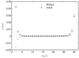
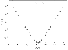
At tree-level $r_{0}(x_{0})$ is $\mathrm{O}((a/L)^{2})$ for all $x_{0}$ for Wilson and for chiral fermions. At 1-loop the behaviour is similar for both discretisaions. There are chiral symmetry breaking effects localised at the boundaries, that survive the continuum limit and decay exponentially with the distance to the boundaries, see fig. 1.

Figure 1: Bare current mass at 1-loop in PT (left). Logarithmic plot of this quantity for chiral fermions (right). The plots are for a $16\times 32$ lattice, $\theta=0$, $N=2$ and $g_{V}^{2}=0$.

5 Renormalised coupling

Having confirmed the desired chiral properties of the proposed chiral fermions in the SF, we now renormalise the couplings at vanishing renormalised mass and define universal quantities that have a finite and unique continuum limit.

To this end we define boundary to boundary correlation functions

$$f_{4}=-\tfrac{a^{4}}{2(N^{2}-1)L^{2}}\sum_{u_{1}v_{1}y_{1}z_{1}}\,\bigl{\langle}\overline{\zeta}^{\prime}(u_{1})\,\gamma_{5}\lambda^{a}\zeta^{\prime}(v_{1})\;\overline{\zeta}(y_{1})\,\gamma_{5}\,\lambda^{a}\zeta(z_{1})\bigr{\rangle}$$ (23)

$$f_{2}=-\tfrac{a^{2}}{NL}\sum_{u_{1}z_{1}}\,\bigl{\langle}\overline{\zeta}(u_{1})\,\zeta^{\prime}(z_{1})\bigr{\rangle}\,,\quad\left(f_{2}\right)_{\mathrm{R}}=Z_{\zeta}^{2}\,f_{2}\quad\text{and}\quad\left(f_{4}\right)_{\mathrm{R}}=Z_{\zeta}^{4}\,f_{4}$$ (24)

and the renormalisation factor free ratio

$$R(\theta)=\frac{\left(f_{4}\right)_{\mathrm{R}}}{\left(f_{2}\right)_{\mathrm{R}}^{2}}-1=\frac{f_{4}}{\left(f_{2}\right)^{2}}-1\quad\text{at}\quad m_{R}=0$$ (25)

which depends on the periodicity angle $\theta$ in the spatial directions. The $\lambda^{a}$s are the generators of the algebra of $SU(N)$ and $\zeta^{\prime}$, $\overline{\zeta}^{\prime}$ are the equivalents of $\zeta$, $\overline{\zeta}$ at $x_{0}=T-a$.

Renormalised couplings can now be defined (up to normalisation factors) as the difference of $R(\theta)$ at two values of $\theta$

$$\tilde{g}^{2}\propto R(\theta_{1})-R(\theta_{2})$$ (26)

and similar for $\tilde{g}_{V}^{2}$ [7]. (The normalisation factors are functions of $\theta_{1}$ and $\theta_{2}$ only and chosen such that in the continuum limit $\tilde{g}^{2}\sim g^{2}$ for small $g^{2}$.) For definiteness we fix one of them to $\theta_{1}=0$. There are then renormalised couplings $\tilde{g}^{2}_{\eta}$, $\tilde{g}_{V,\eta}^{2}$ for each value $\theta_{2}=\eta$. They have an expansion in PT and the 1-loop result for $\tilde{g}_{\eta}^{2}$ with the proper normalisation is

$$\tilde{g}^{2}_{\eta}\stackrel{{\scriptstyle a\to 0}}{{=}}g^{2}_{w}+g^{4}_{w}\,b_{0}\,\ln(a/L)+c_{g}^{w}(\eta)+\mathrm{O}(g^{6})$$ (27)

for Wilson fermions and

$$\tilde{g}^{2}_{\eta}\stackrel{{\scriptstyle a\to 0}}{{=}}g^{2}_{gw}+g^{4}_{gw}\,b_{0}\,\ln(a/L)+c_{g}^{gw}(\eta)+\mathrm{O}(g^{6})\,,$$ (28)

for chiral (gw) fermions. In this formulae, $b_{0}=-N/\pi$, is the correct universal first coefficient of the beta-function (showing asymptotic freedom), which was computed earlier in the continuum [12]. The finite parts found in the two computations differ as expected. The result for the renormalised couplings $\tilde{g}_{V}^{2}$, corresponding to the vector-vector interaction, can be found in ref. [7]. We here only note, that after rearranging the terms in the action with the help of Fierz-transformations, this coupling has (up to 1-loop) a vanishing beta-function.

An universal renormalisation group invariant (RGI) quantity can now be defined as the difference of the renormalised coupling for two different values of $\eta$. This is because in the continuum a non-zero $\theta$ in (3) shifts the momenta of the external legs, but does not effect the loop integrals. The difference

$$F_{\mathrm{RGI}}(\eta,a/L)=\tilde{g}^{2}_{\eta}(a/L)-\tilde{g}^{2}_{\eta_{0}}(a/L)\,,\quad\eta_{0}=1\,.$$ (29)

has an expansion in the renormalised couplings (we omit the subscript $\eta$)

$$F_{\mathrm{RGI}}(\eta,a/L)=F^{(1)}_{1}(\eta,a/L)\,\tilde{g}^{4}+F^{(1)}_{2}(\eta,a/L)\,\tilde{g}^{2}\,\tilde{g}^{2}_{V}+F^{(1)}_{3}(\eta,a/L)\,\tilde{g}_{V}^{4}+\mathrm{O}(\tilde{g}^{6})\,,$$ (30)

where the coefficients are given by the finite parts. Since it is an universal quantity, these coefficients have a finite and unique continuum limit independent of the discretisation.

$\eta$	0.1	0.2	0.3	0.4	0.5
$F^{(1)}_{1,\mathrm{w}}(\eta,0)$	5.0797(6)	4.4704(5)	3.6395(3)	2.7629(1)	1.9672(1)
$F^{(1)}_{1,\mathrm{gw}}(\eta,0)$	5.078(2)	4.469(2)	3.638(2)	2.762(2)	1.966(2)

Table 1: First order coefficients in the expansion of $F_{\mathrm{RGI}}$ with Wilson (w) and chiral (gw) fermions.

The continuum values for different choices of $\eta$ are given in tab. 1. The errors are estimated by fitting the first few terms of the Symanzik expansion of lattice diagrams to the data at lattice sizes from $4\times 8$ to $64\times 128$ ($128\times 256$) for chiral (Wilson) fermions (method explained in appendix D of [13]). The continuum values agree within the error, thus confirming universality for the operator (5).

6 Final remarks

The formulation of the SF for fermionic models of the Gross-Neveu type in [7] has enabled the first test of the recently proposed chiral Dirac operator in the presence of the SF boundary conditions. At 1-loop we have shown that a chiral Ward identity takes its continuum value far away from the boundaries. The calculation of an universal quantity gives the right discretisation independent value.

The size of the lattice artifacts has not been discussed so far. What we observe is that the chiral fermions are tree-level $\mathrm{O}(a)$-improved, if the value of $c$ is tuned correctly. At 1-loop it is not enough to tune $c$, because there are dimension 3 operators at the boundary, that spoil automatic $\mathrm{O}(a)$-improvement. This however is peculiar to the studied kind of models with four-fermion interactions.

As next step, it would be desirable to perform a similar (perturbative) computation in QCD in order to provide guidance for the final non-perturbative application of chiral fermions in the Schrödinger functional.

Acknowledgement

We would like to thank Rainer Sommer for critical reading an early version of the text. This work was supported by Deutsche Forschungsgemeinschaft in form of Sonderforschungsbereich SFB TR 09.

References

- [1] M. Luscher, JHEP 0605 (2006) 042 [arXiv:hep-lat/0603029].
- [2] D. J. Gross and A. Neveu, Phys. Rev. D 10 (1974) 3235.
- [3] R. Sommer, Nucl. Phys. Proc. Suppl. 160 (2006) 27 [arXiv:hep-ph/0607088].
- [4] S. Sint, Nucl. Phys. B 421 (1994) 135, Nucl. Phys. B 451 (1995) 416
- [5] S. Sint, PoS LAT2005 (2006) 235 [arXiv:hep-lat/0511034].
- [6] P. H. Ginsparg and K. G. Wilson, Phys. Rev. D 25 (1982) 2649.
- [7] B. Leder, PhD Thesis, arXiv:0707.1939 [hep-lat].
- [8] M. Luscher, S. Sint, R. Sommer and P. Weisz, Nucl. Phys. B 478 (1996) 365 [arXiv:hep-lat/9605038].
- [9] P. Hernandez, K. Jansen and M. Luscher, Nucl. Phys. B 552, 363 (1999) [arXiv:hep-lat/9808010].
- [10] L. Giusti et al., Comput. Phys. Commun. 153 (2003) 31 [arXiv:hep-lat/0212012].
- [11] M. Luscher, Phys. Lett. B 428 (1998) 342 [arXiv:hep-lat/9802011].
- [12] P. K. Mitter and P. H. Weisz, Phys. Rev. D 8 (1973) 4410.
- [13] A. Bode, P. Weisz and U. Wolff [ALPHA collaboration], Nucl. Phys. B 576 (2000) 517