Finite-size correction in many-body electronic structure calculations

Abstract

Finite-size (FS) effects are a major source of error in many-body (MB) electronic structure calculations of extended systems. A method is presented to correct for such errors. We show that MB FS effects can be effectively included in a modified local density approximation calculation. A parametrization for the FS exchange-correlation functional is obtained. The method is simple and gives post-processing corrections that can be applied to any MB results. Applications to a model insulator (P₂ in a supercell), to semiconducting Si, and to metallic Na show that the method delivers greatly improved FS corrections.

Realistic many-body (MB) calculations for extended systems are needed to accurately treat systems where the otherwise successful density functional theory (DFT) approach fails. Examples range from strongly correlated materials, such as high-temperature superconductors, to systems with moderate correlation, for instance where accurate treatments of bond-stretching or bond-breaking are required. DFT or Hartree Fock (HF), which are effectively independent-particle methods, routinely exploit Bloch’s theorem in calculations for extended systems. In crystalline materials, the cost of the calculations depends only on the number of atoms in the periodic cell, and the macroscopic limit is achieved by a quadrature in the Brillouin zone, using a finite number of ${\mathbf{k}}$-points. MB methods, by contrast, cannot avail themselves of this simplification. Instead calculations must be performed using increasingly larger simulation cells (supercells). Because the Coulomb interactions are long-ranged, finite-size (FS) effects tend to persist to large system sizes, making reliable extrapolations impractical. The resulting FS errors in state-of-the-art MB quantum simulations often can be more significant than statistical and other systematic errors. Reducing FS errors is thus a key to broader applications of MB methods in real materials, and the subject has drawn considerable attention Kent et al. (1999); Chiesa et al. (2006).

In this paper, we introduce an external correction method, which is designed to approximately include FS corrections in modified DFT calculations with finite-size functionals. The method is simple, and provides post-processing corrections applicable to any previously obtained MB results. Conceptually, it gives a consistent framework for relating FS effects in MB and DFT calculations, which is important if the two methods are to be seamlessly interfaced to bridge length scales. The correction method is applied to a model insulator (P₂ in a supercell), to semiconducting bulk Si, and to Na metal. We find that it consistently removes most of the FS errors, leading to rapid convergence of the MB results to the infinite system.

We write the ${\mathcal{N}}$-electron MB Hamiltonian in a supercell as (Rydberg atomic units are used throughout):

$$H=-\sum_{i=1}^{\mathcal{N}}\nabla_{i}^{2}+\sum_{i=1}^{\mathcal{N}}V_{\mathrm{ion},i}+\sum_{i<j}V^{\rm FS}(|{\bf r}_{i}-{\bf r}_{j}|)\,,$$ (1)

where the ionic potential on $i$ can be local or non-local, and ${\bf r}_{i}$ is an electron position. The Coulomb interaction $V^{\rm FS}$ between electrons depends on the supercell size and shape, due to modification by the periodic boundary conditions (PBC) Fraser et al. (1996). A FS correction is often applied to the MB results from parallel DFT or HF calculations. The corresponding DFT, as usually formulated, introduces a fictitious mean-field ${\mathcal{N}}$-electron system Hohenberg and Kohn (1964); Kohn and Sham (1965):

$$H_{\rm DFT}=-\nabla^{2}+V_{\mathrm{ion}}+V_{H}({\bf r})+V_{xc}^{\infty}({\bf r})\,,$$ (2)

where the Hartree and exchange-correlation (XC) potentials depend self-consistently on the electronic density $n({\bf r})$. In the non-spin-polarized local density approximation (LDA), for example: $V_{xc}^{\infty}({\bf r})=\delta(n({\bf r})\,\epsilon_{xc}^{\infty}(n))/\delta n({\bf r})$, where $\epsilon_{xc}^{\infty}(n)$ is typically obtained from quantum Monte Carlo (QMC) results on the homogeneous electron gas (jellium), extrapolated to infinite size Ceperley (1978); Ceperley and Alder (1980); Perdew and Zunger (1981).

Residual errors after DFT FS correction are still found to be large, however, and the equations above illustrate why. The jellium QMC results, which determine $\epsilon_{xc}^{\infty}(n)$, have been extrapolated to infinite supercell size for each density. This is the correct choice for standard LDA applications, where Bloch’s theorem will be used to reach the infinite limit. It is not ideal, however, if the LDA is expected to provide FS corrections. Only one-body FS corrections (kinetic, Hartree, etc), which arise from incomplete ${\bf k}$-point integration, are included, while two-body FS corrections Kent et al. (1999) are missing. If parallel HF calculations are used instead, exact FS exchange $V_{x}\rightarrow V_{x}^{\rm FS}$ is included, but $V_{c}$ is zero.

Our approach is to construct an LDA with FS XC in Eq. (2). If the supercell of Eq. (1) is cubic (for simplicity), the XC energy is $\epsilon^{\mathrm{FS}}_{xc}(n)\equiv\epsilon_{x}(r_{s},L)+\epsilon_{c}(r_{s},L)$, where $r_{s}$ specifies the density via $4\pi r_{s}^{3}/3\equiv 1/n$ and $L$ denotes the linear size of the supercell. To obtain $\epsilon^{\mathrm{FS}}_{xc}(r_{s},L)$, we use unpolarized jellium systems in the same supercell, in which the number of electrons $N$ (distinct from ${\mathcal{N}}$) is a variable Fou , given by the ratio $r_{s}/L$: $N=(3/4\pi)(L/r_{s})^{3}$.

We parametrize the HF exchange energy in jellium by:

$$\epsilon_{x}(r_{s},L)=\cases{\frac{a_{0}}{r_{s}}+\frac{a_{1}}{L^{2}}r_{s}+\frac{a_{2}}{L^{3}}r_{s}^{2},&if $r_{s}\leq\gamma$;\cr\frac{a_{3}L^{5}}{r_{s}^{6}},&other.\cr}$$ (3)

The term with $a_{0}\simeq-0.916\,$Ry gives the usual infinite-size limit. A $1/L$ canceling term, which arises from the self-interaction of an electron with its periodic images Fraser et al. (1996), has been implicitly included. The leading FS dependence is then $1/L^{2}$ Ceperley (1978). The form of the remaining terms is motivated by the exact scaling relation: $\epsilon_{x}(r_{s},L)=\widetilde{\epsilon}_{x}(N)/L$. To obtain $\epsilon_{x}$, we calculate $\widetilde{\epsilon}_{x}(N)$ for a range of $N$, each by averaging over about 20 $\mathbf{k}$-points. The results are fitted to give $a_{1}$ and $a_{2}$. As illustrated in Fig. 1, the quality of the fit is excellent. The behavior of $\epsilon_{x}$ at large $r_{s}$ requires special handling for finite $L$. At $\gamma\equiv r_{s}(N=2)$, there is only one electron of each spin in the supercell, so $\epsilon_{x}$ is just the self-interaction term. Beyond $\gamma$, $\epsilon_{x}$ is forced to go to zero as $1/r_{s}^{6}$, reflecting the self-interaction of a ‘fractional’ electron. The coefficient $a_{3}$ is chosen to make the exchange potential $V_{x}^{\rm FS}$ continuous at $\gamma$ foo . From Fig. 1, the magnitude of the discontinuity at $r_{s}=\gamma$ is seen to decrease with increasing $L$, as expected. All parameters are listed in Table 1.

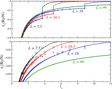
Figure 1: (Color online) Calculated and parametrized jellium exchange and correlation energies per electron vs. $r_{s}$, for a range of supercell sizes $L$ (in Bohr). Top panel: exchange energies, with solid lines given by the fit in Eq. (3), and open symbols by ${\bf k}$-point averaged calculations. Bottom panel: correlation energies, with solid lines given by the fit in Eq. (6), open symbols by AF QMC calculations, and small filled symbols by the large-$N$ asymptotic expression in Eq. (5).

Table 1: Parameters (in Ry atomic units) in the FS XC functionals.

$i$	1	2	3	4
$a_{i}$ [Eq. (3)]	$-2.2037$	$0.4710$	$-0.0150$	—
$g_{i}$ [Eq. (6)]	$0.1182$	$1.1656$	$-5.2884$	$-1.1233$

The correlation energy in jellium is the difference between the MB and HF energies (per electron):

$$\epsilon_{c}(r_{s},L)=\mathcal{E}(r_{s},L)-t(r_{s},L)-\epsilon_{x}(r_{s},L),$$ (4)

where the jellium non-interacting kinetic energy obeys the scaling relation $t(r_{s},L)=\widetilde{t}(N)/L^{2}$. We calculate $\widetilde{t}(N)$ in the same way as $\epsilon_{x}(r_{s},L)$, but averaging over more $\mathbf{k}$-points to ensure convergence.

We next derive the MB energy $\mathcal{E}$. Ceperley and Alder Ceperley and Alder (1980) obtained jellium QMC energies for various values of $N$ and provided the following fit:

$$\mathcal{E}(r_{s},L)=\mathcal{E}^{\infty}(r_{s})+b_{1}(r_{s})\Delta t_{N}+b_{2}(r_{s})/N,$$ (5)

where $N$ uniquely determines $L$, and $\Delta t_{N}=t(r_{s},L)-t(r_{s},\infty)$ is the FS error in the free-electron kinetic energy. The infinite-size limit, $\mathcal{E}^{\infty}$, was extrapolated from Eq. (5) and it is the basis for $V_{xc}^{\infty}$ in Eq. (2). The $b$ parameters were given for several $r_{s}$ values, which we fit to get the functions $b_{1}(r_{s})$ and $b_{2}(r_{s})$. With these and $\Delta t_{N}$, we can now calculate $\mathcal{E}(r_{s},L)$ for any $r_{s}$ and $L$, which is accurate for large $N$.

For small $N$, namely large $r_{s}$ in a finite supercell, Eq. (5) does not apply. This is easy to see from the $1/N$ term which, at sufficiently large $r_{s}$, causes $\epsilon_{c}$ to diverge. To guide the analysis in this region, we use the plane-wave auxiliary-field (AF) QMC method Zhang and Krakauer (2003); Suewattana et al. (2007) to directly calculate $\mathcal{E}$ for FS jellium systems. At small $r_{s}$, the correlation energy obtained is in excellent agreement with that derived from Eq. (5), as shown in Fig. 1. At large $r_{s}$, $\epsilon_{c}$ from Eq. (5) falls below the AF QMC value [$b_{2}(r_{s})$ is negative], as the latter goes to zero monotonically. The value of $r_{s}$ where the two begin deviating depends on $L$, since it is determined by $N$.

We thus parametrize the correlation energy by

$$\epsilon_{c}(r_{s},L)=\cases{\epsilon_{c}^{\infty}(r_{s})-\frac{a_{1}}{L^{2}}r_{s}+\frac{g(r_{s})}{L^{3}},&$r_{s}\leq\gamma_{h}$;\cr f(r_{s}),&$\gamma_{h}<r_{s}\leq\gamma_{l}$;\cr 0,&other.\cr}$$ (6)

The correlation functional has been divided into high, intermediate, and low density regions. The boundaries are defined by $\gamma_{h}\equiv r_{s}(N=12)$ and $\gamma_{l}\equiv r_{s}(N=1/2)$, which are guided by the discussion in the previous paragraph and the quality of the fits described below, but are otherwise arbitrary. At high densities, the infinite-size limit is given by $\epsilon_{c}^{\infty}(r_{s})$ (the Perdew-Zunger parametrization Perdew and Zunger (1981) is used here), and the leading FS term exactly cancels that in $\epsilon_{x}(r_{s},L),$ to ensure that $\epsilon_{xc}(r_{s},L)$ correctly scales as ${\mathcal{O}}(1/L^{3})$. The function $g(r_{s})\equiv g_{1}r_{s}\ln(r_{s})+g_{2}r_{s}+g_{3}r_{s}^{3/2}+g_{4}r_{s}^{2}$ is obtained from a fit to $\epsilon_{c}(r_{s},L)$ from Eqs. (4) and (5). (The fits are illustrated in Fig. 1 and parameters are given in Table 1.) At intermediate densities, the function $f(r_{s})$ is given by a cubic polynomial and is completely determined by the requirement that $\epsilon_{c}$ and its derivative be continuous at $r_{s}=\gamma_{h}$ and $r_{s}=\gamma_{l}$. As Fig. 1 shows, the parametrization in Eq. (6) closely reproduces our AF QMC data at low densities for all cell sizes.

Post-processing FS corrections are now easily generated for any MB calculation. The DFT^FS results, using $\epsilon^{\mathrm{FS}}_{xc}$ from Eqs. (3) and (6), can be obtained from standard DFT computer codes with only minor modifications. If $E^{\mathrm{FS}}(L)$ is the energy from DFT^FS and $E(L)$ from standard DFT (i.e., DFT^∞), the energy correction is $\Delta\mathrm{DFT}^{\mathrm{FS}}=E(\infty)-E^{\mathrm{FS}}(L)$, where $E(\infty)$ is obtained by ${\bf k}$-point integration. The correction can alternatively be expressed as the sum of $\Delta\mathrm{DFT}^{\mathrm{1B}}\equiv E(\infty)-E(L)$ and $\Delta\mathrm{DFT}^{\mathrm{2B}}\equiv E(L)-E^{\mathrm{FS}}(L)$. The one-body (1B) correction is the usual $\Delta\mathrm{DFT}^{\infty}$, while the two-body (2B) part captures the FS effects that arise from the modification of $V_{xc}$ due to supercell PBC.

The present correction scheme is exact for homogeneous systems. Our first application of the method is to a model system in the opposite limit. We consider a “molecular solid” with P₂ in a periodic supercell, treated by the plane-wave AF QMC method Zhang and Krakauer (2003); Suewattana et al. (2007). Because of the low-density “vapor” region and the variation in density, the system provides a challenging test for the correction method. A norm-conserving Kleinman-Bylander Kleinman and Bylander (1982) separable non-local LDA pseudopotential is used OPI . Total energy calculations were performed at the equilibrium bondlength of 3.578 Bohr, for cubic supercells of size $L=7-18$ Bohr, all with the $\Gamma$-point ($\mathbf{k}=0$). Figure 2 shows the results from AF QMC and LDA using both DFT^∞ and DFT^FS Gonze and et al. (2002). The uncorrected QMC result has large FS errors and, at $L=18$, is still $\sim$ 0.3 eV away from the infinite-size value. Corrected with DFT^∞, the FS error is somewhat reduced at intermediate $L$, but is unchanged for larger $L$ where the 2B effects dominate. With the new method, the corrected energy shows excellent convergence across the range, reaching the asymptotic value (within statistical errors) by $L\sim 12$.

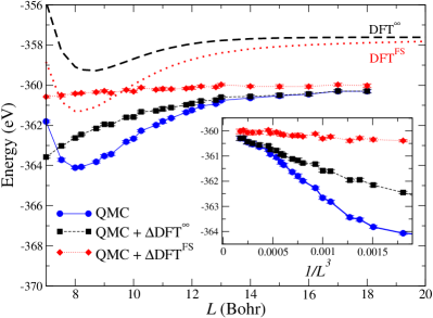
Figure 2: (Color online) $P_{2}$ PBC total energy convergence vs. supercell size. Standard DFT^∞ FS effect is different (too small) from that of MB AF QMC. DFT^FS parallels the MB calculation and leads to much more rapid convergence. The inset focuses on larger $L$ and shows the raw and corrected AF QMC results plotted as a function of $1/L^{3}$.

The second application is for fcc bulk silicon, using non-cubic supercells ($n\!\times\!n\!\times\!n$ the size of the primitive fcc cell). The raw MB energies in Fig. 3 are taken from diffusion Monte Carlo (DMC) calculations Kent et al. (1999). In the FS corrections for the fcc supercells, we use $\epsilon_{xc}^{\mathrm{FS}}$ from Eqs. (3) and (6), with an effective $L$ equal to the size of a cubic supercell of the same volume. The pseudopotential used is also different from that in the DMC calculations. We checked multiple pseudopotentials to ensure that the FS corrections are independent of the choice of pseudopotential. The DMC calculations were done with the $\mathbf{k}=\mathrm{L}$ point. The usual DFT correction is in the wrong direction in this case, thereby increasing the FS error. The new method removes most of the error, despite the non-optimal $\epsilon_{xc}^{\mathrm{FS}}$. The inset in Fig. 3 shows $\Delta\mathrm{DFT}^{\mathrm{2B}}$ calculated as above for fcc, compared with that for cubic supercells. Both are seen to fall on an essentially smooth and linear curve. This weak shape dependence of $\epsilon_{xc}^{\mathrm{FS}}$ is encouraging, suggesting that additional FS MB jellium calculations can be avoided in some non-cubic supercells.

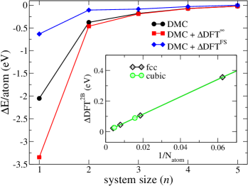
Figure 3: (Color online) Total energy per atom (in eV) of bulk Si in fcc supercells of size $n\!\times\!n\!\times\!n$ ($2n^{3}$ atoms). DMC energies in the main graph are from Kent et. al. Kent et al. (1999) (shifted here relative to the extrapolated infinite-size limit). FS corrections are shown from both standard DFT and the present method. The inset shows the calculated two-body correction as a function of inverse the number of atoms, for fcc and cubic supercells.

The final application is for metallic bcc bulk Na. While in insulators a single ${\mathbf{k}}$-point is often adequate, metals present additional difficulties. We do multiple MB calculations with random ${\mathbf{k}}$-points (e.g. 50 for 16 atoms) and average the results Lin et al. (2001). The plane-wave AF QMC method Zhang and Krakauer (2003); Suewattana et al. (2007) was used, in which any ${\mathbf{k}}$-point can be included by a simple modification to the one-particle basis. Although our pseudopotential has a Ne-core, DFT tests with various pseudopotentials verified that it is sufficient for the cohesive energy (consistent with Ref. Maezono et al. (2003)), but the frozen semi-core introduces systematic biases in the lattice constant and bulk modulus.

Table 2: Calculated cohesive energy (in eV) of bcc solid sodium vs. experiment. AF QMC results from supercells with 2, 16 and 54 atoms are shown, together with FS-corrected results. A zero-point energy of $0.0145$ eV/atom is included. Experimental value was taken from Ref. Maezono et al. (2003).

		corrected
	raw	w/ 1-body	w/ full FS
$2$	$2.050(35)$	$2.141(2)$	$1.124(2)$
$16$	$1.264(14)$	$1.287(4)$	$1.135(4)$
$54$	$1.184(9)$	$1.189(10)$	$1.143(10)$
expt			$1.129(6)$

The calculated cohesive energies are given in Table 2. The FS-corrected cohesive energies for 16 and 54 atoms are consistent, and in better agreement with experiment than the previous best DMC results Maezono et al. (2003) of $1.0221(3)$ eV (with a core polarization potential) and $0.9910(5)$ eV (without). The calculated equation of state is shown in Fig. 4. We see that, with the new FS corrections and ${\mathbf{k}}$-point sampling, the calculations have better convergence than previously reachable with an order of magnitude larger system sizes Maezono et al. (2003). Both the lattice constant and the bulk modulus were modified by the FS corrections. As the bottom panel demonstrates, FS effects always cause a systematic error in the lattice constant in uncorrected MB calculations.

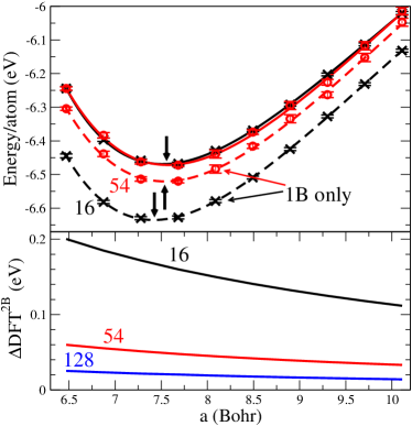
Figure 4: (Color online) Top: Equation of state for bcc Na. The AF QMC energy is shown vs. lattice constant $a$ for 16- and 54-atom supercells, with one-body (1B) and full FS corrections. With full correction (solid lines), 16- and 54-atom results are almost indistinguishable. QMC statistical errors include that of ${\mathbf{k}}$-point averaging. The vertical arrows indicate the calculated equilibrium $a$. Bottom: persistence of the two-body FS error, with finite slopes (number of atoms indicated).

These tests show that our DFT^FS correction method works well in a variety of systems. This is perhaps not surprising, given the often near-sighted nature of the XC function. For the method to be effective, DFT needs to provide a good approximation in capturing the difference between the systems with interaction $V^{\rm FS}$ and $V$, which is not the same as requiring DFT to work well in either system (assuming $L$ greater than the size of the XC hole). We have presented an XC functional which delivers high accuracy across several different materials. Previous attempts at FS correction have focused on estimating the errors internally within the MB simulation Kent et al. (1999); Chiesa et al. (2006). Our approach is an external method which is simple and can provide post-processing FS correction to any MB electronic structure calculations. The method can be generalized, e.g., to spin-polarized systems and other supercell shapes, and the FS functional could be further improved, e.g., by exact exchange.

We thank E. J. Walter for help with pseudopotentials, W. Purwanto for help with computing issues, and P. Kent for sending us the numerical data from Ref. Kent et al. (1999). This work is supported by ONR (N000140510055), NSF (DMR-0535529), and ARO (48752PH) grants. Computing was done on NERSC and CPD computers.

References

- Kent et al. (1999) P. R. C. Kent et. al., Phys. Rev. B 59, 1917 (1999).
- Chiesa et al. (2006) S. Chiesa et. al., Phys. Rev. Lett. 97, 076404 (2006).
- Fraser et al. (1996) L. M. Fraser et. al., Phys. Rev. B 53, 1814 (1996).
- Hohenberg and Kohn (1964) P. Hohenberg and W. Kohn, Phys. Rev. 136, B864 (1964).
- Kohn and Sham (1965) W. Kohn and L. J. Sham, Phys. Rev. 140, A1133 (1965).
- Ceperley (1978) D. M. Ceperley, Phys. Rev. B 18, 3126 (1978).
- Ceperley and Alder (1980) D. M. Ceperley and B. J. Alder, Phys. Rev. Lett. 45, 566 (1980).
- Perdew and Zunger (1981) J. P. Perdew and A. Zunger, Phys. Rev. B 23, 5048 (1981).
- (9) In M. Nekovee et. al., Phys. Rev. B 68, 235108 (2003), finite-size LDA calculations modified to incorporate the effect of a fixed number of electrons were mentioned.
- (10) In crystalline systems, the contribution from is negligible for any reasonable size and we use a constant to make continuous.
- Zhang and Krakauer (2003) S. Zhang and H. Krakauer, Phys. Rev. Lett. 90, 136401 (2003).
- Suewattana et al. (2007) M. Suewattana et. al., Phys. Rev. B 75, 245123 (2007).
- Kleinman and Bylander (1982) L. Kleinman and D. M. Bylander, Phys. Rev. Lett. 48, 1425 (1982).
- (14) Generated with OPIUM: http://opium.sorceforge.net.
- Gonze and et al. (2002) X. Gonze et. al., Comput. Mat. Sci. 25, 478 (2002); all LDA calculations were performed with ABINIT: http://www.abinit.org.
- Lin et al. (2001) C. Lin et. al., Phys. Rev. E 64, 016702 (2001).
- Maezono et al. (2003) R. Maezono et. al., Phys. Rev. B 68, 165103 (2003).