Revolving rivers in sandpiles: from continuous to intermittent flows

Abstract

In a previous paper [Phys. Rev. Lett. 91, 014501 (2003)], the mechanism of “revolving rivers” for sandpile formation is reported: as a steady stream of dry sand is poured onto a horizontal surface, a pile forms which has a river of sand on one side flowing from the apex of the pile to the edge of the base. For small piles the river is steady, or continuous. For larger piles, it becomes intermittent. In this paper we establish experimentally the “dynamical phase diagram” of the continuous and intermittent regimes, and give further details of the piles “topography”, improving the previous kinematic model to describe it and shedding further light on the mechanisms of river formation. Based on experiments in Hele-Shaw cells, we also propose that a simple dimensionality reduction argument can explain the transition between the continuous and intermittent dynamics.

I Introduction

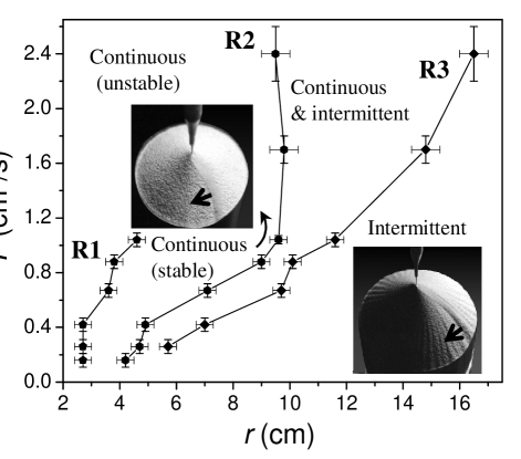
Figure 1: Occurrence of continuous and intermittent rivers, as function of the pile radius $r$ and the input flux $F$. The upper and lower insets show snapshots of the pile during the (stable) continuous and the intermittent regimes, respectively. The arrows indicate the direction of revolution around the pile

When most granular materials are poured onto a horizontal surface, a conical pile builds up through an avalanche mechanism involving all the surface of the pile that “tunes” the angle of repose about a certain critical value. In a previous paper, however, we reported a different mechanism of sandpile formation Altshuler2003 . In those experiments, as the pile grows, a river of sand spontaneously builds up, flowing down one side of the pile from the apex to the base. The river then begins to revolve around the pile, depositing an helical layer of material with each revolution, causing the pile to grow. Below a certain pile size and input flux, the rivers are continuous, and the surface of the pile is smooth (see upper inset in Fig. 1). The revolving direction can be either clockwise or counterclockwise, only depending on random fluctuations in the first stage of the experiment. For bigger piles, the rivers are intermittent, and the surface of the pile become undulated (see lower inset in Fig. 1). X.-Z. Kong and coworkers Kong2006 reported a detailed computational model for the revolving rivers which manages to reproduce many of their features in the continuous regime, but the intermittent regime was not accounted for. They also noticed that the details of the grain-grain interactions must be tuned in order to get the revolving rivers, which matches the experimental fact that not all sands display such behavior. In this paper, we explore experimentally the “dynamic phase diagram” of the different regimes in our sandpiles (i.e., the regions of experimental parameters where they appear). We report the details of the “topography” of the sandpiles in the continuous and intermittent regimes, and present a refined “kinetic” description of the observed phenomena. We then propose an explanation for the existence of two types of revolving rivers based on an analogy with measurements performed in a simpler geometry (i.e., the Hele-Shaw cell).

II The “dynamic phase diagram” of the revolving rivers

We used sand with a high content of silicon oxide from Santa Teresa (Pinar del Río, Cuba) Altshuler2003 ; Etien2007 . The grain size distribution is basically a Gaussian distribution centered at $200\mu$m, with a half-width slightly smaller than $200\mu$m. From now on, we will adopt the labelling of reference Altshuler2003 for the boundary conditions used in each experiment: BCI stands for a pile grown on a closed cylindrical container with a flat, horizontal bottom (like a glass of rum), and BCII corresponds to a pile formed on an open, flat horizontal surface. To obtain the dynamic phase diagram, we grew piles in boundary condition BCII. We used glass funnels of various diameters to obtain different values of the input flux. It was determined in each experiment by measuring the volume of the conical pile, and dividing it by the time elapsed since the first grains were dropped on the table. For a given input flux, three different pile base radii where identified by simple observation as the pile grew. Below $r1$, continuous rivers appeared and disappeared (as eventually happens in common sands), so we will refer to them as unstable. Above $r1$ and below $r2$, a stable continuous river revolved around the pile in a given direction, without any major changes in its shape. After $r2$, the continuous river could eventually become intermittent: the downhill flow would suddenly stop at the edge of the pile, and a “finger” of sand would escalate from bottom to top, like a “stop-up” front Douady2000 . All in all, the continuous or intermittent rivers would keep revolving around the pile with the frequency described in Altshuler2003 (see also Fig. 7). However, at some point this process transformed again into a continuous, revolving river. As the radius of the pile grew from $r2$ to $r3$, the intermittent mechanism took place within larger and larger time intervals, while the continuous mechanism slowly disappeared. At $r3$, intermittent rivers where established as the only dynamical phase in the pile. As $r1$, $r2$ and $r3$ were determined for various input fluxes, three boundaries $R1$, $R2$ and $R3$ were established to separate the different dynamical phases, as shown in Fig. 1. We have observed that the positions of these lines are influenced by the distance between the funnel that delivers the sand and the tip of the pile, but we kept this distance fixed at approximately $2$ cm during the experiments. It should be noticed that, for input fluxes bigger than approximately $1cm^{3}/s$, stable continuum rivers are never established, and a direct transition from unstable continuous to intermittent rivers takes place through $R2$.

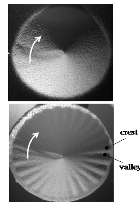
Figure 2: Topography of the continuous and intermittent regimes. Upper panel: top view showing a pile “frozen” during a continuous river experiment. The diameter of the pile is $11$cm. Lower panel: top view of a pile “frozen” during an intermittent river experiment. The diameter of the pile is $17$cm –surface undulations extend approximately $6$ cm from the edge of the pile in the radial direction. Black arrows on top of the flowing river indicate the direction of revolution of the rivers as sand is added from above.

III Refined kinematic model

Figure 2 shows images taken from top of “frozen” piles in the stable continuous (upper panel) and intermittent (lower panel) regimes obtained for boundary condition BCII. Piles were formed using a steady input flux, which was just switched off to take the pictures. In both images, the river can be identified as a curved groove from the apex to the base of the pile, in a general vertical direction, below the apex. In order to quantify the topography of the piles (at least for one size), we measured its slope angle (polar angle) versus the angle around the pile (azimuthal angle). The measurement was performed by carefully setting a ruler tangential to the slope of the pile at different azimuthal angles, taking a lateral picture of the system, and calculating the angles between the ruler and the horizontal from the resulting images. This ruler was set along the section of the slope where the angle is essentially constant (this angle becomes smaller at a few cm from the top of the piles). Figure 3 shows how the slope angle depends on the azimuthal angle for the case of the continuous rivers. Contrary to the first impression when the picture of the upper panel of Fig. 2 is examined, there is a wide angular zone of variation of the slope angle, quantified in Fig. 3. This suggests that, while most of the downhill flow is concentrated into the relatively narrow river clearly visible below the apex of the pile (upper panel of Fig. 2), there is a wider area of grains rolling downhill. The slope angle is typically around 36.5 degrees far from the river. It significantly decreases to 33 degrees within the river. The width of the low slope angle region extends over $150$ degrees along the azimuthal direction. This corresponds to a length of around $28$ cm along the circumference of the pile, which is much larger than the river (which is a few cm wide). To illustrate this, Figure 4 shows the difference between two images of a sandpile grown in BCI in the continuous regime, separated by a lapse of $0.15$ seconds (the video was taken by a Photon Fastcam Ultima-ADX model 120K, and the image was obtained using the “difference” option of ImageJ). Besides the fast flow along the main stream of the river, whiter and darker spots indicate the downhill movement of sand at a smaller speed behind the main stream area.

The situation is quite different in the case of the intermittent regime. The measurement of the angles of repose of several “valleys” and “crests” corresponding to the picture in the lower panel of Fig. 2 does not indicate a wide transition in the angle of repose, as in the case of the continuous rivers, but suggests two basic polar angles: $37.1\pm 0.16$ degrees, for the valleys, and $36.1\pm 0.20$ degrees for the crests. It should be noticed, however, that the pile in the intermittent regime contains an inner circle where the surface is smooth, and an outer ring of undulating surface, as seen in Fig. 2 (lower panel). The values we have reported here for the slope angles at the valleys and crests correspond to this ring of approximately $6$ cm width in the radial direction, while the average slope of the pile in the inner circle is harder to measure due to rounding near the apex of the pile.

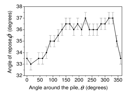
Figure 3: Dependence of the angle of repose on the azimuthal angle for the picture of the upper panel of Fig. 2 (continuous river). The “0” of the azimuthal angle has been taken along the vertical diameter under the apex, and it increases clockwise. The error bars correspond to the largest variation of the measured angles of repose in three different attempts on the same pile.

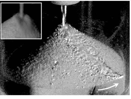
Figure 4: Moving grains in the continuous river regime. The figure is the difference between two pictures of a continuous river separated by $0.15$ seconds (the river was revolving around the pile at approximately $0.1$ turns/s). This difference is superimposed with the first of these two pictures. The arrow indicates the direction of the revolution of the river around the pile. The inset shows a raw picture of the crater, at the upper end of the pile.

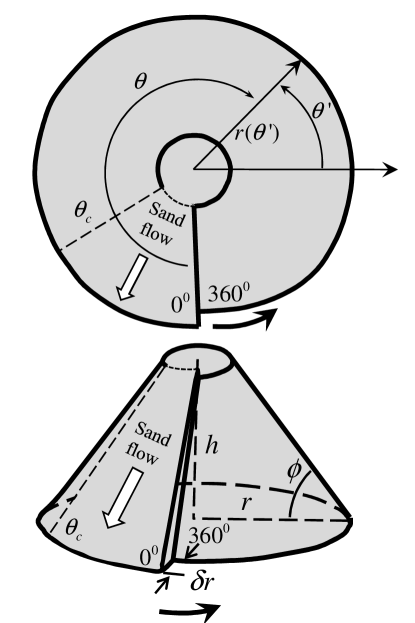
Figure 5: Diagram of the model used to estimate the revolving speed of the rivers, and the polar bottom angle versus the azimuthal angle. Upper panel: top view of the pile model. Lower panel: spatial view of the pile model (notice that the angle of the flowing zone has been decreased in this representation relative to the top view, to improve drawing clarity). The black arrows indicate the direction of revolution around the pile.

The phenomenological model for the revolving rivers presented in reference Altshuler2003 is able to predict the radius and time dependence of the frequency of revolution of the piles, but oversimplifies the geometry of the sandpile in such a way that the angle of repose is constant around the pile, in contradiction with the real topography shown in Fig. 2 and quantified in Fig. 3. We present here a more realistic model, which is schematized in Fig. 5 for BCII. This model has a number of advantages relative to the one presented in reference Altshuler2003 . First, it takes into account that the apex of the pile is not sharp, but presents a small “crater” (very exaggerated in the schematics shown in Fig. 5). Second, the river, located in the section on the cone on which the sand flows, has a nonzero width. Third, the angle of repose is not constant around the pile, but can be shaped as depicted in Fig. 5, where the width of the downhill flowing area has been tuned to $150$ degrees in the azimuthal direction (the figure displays a smaller angle). We add two further constraints, which roughly match experimental observations: the characteristic length $\delta$r is constant, and so is the radius of the crater.

The geometry of the pile, in the continuous regime, can be schematized as follows:

We define an azimuthal coordinate $\theta$ around the pile in a frame co-moving with the revolving river, so that $\theta=0$ corresponds to the position of the flowing river, where most of the flow is located. In the reference frame of the laboratory, the azimuthal coordinate $\theta^{\prime}$ is $\theta^{\prime}=\theta_{0}(t)-\theta$, where $\theta_{0}(t)=\theta_{0}(0)+\int_{0}^{t}\omega(t^{\prime})dt^{\prime}$ is the azimuthal angle of the river, and $\omega(t)=\dot{\theta}_{0}(t)$ is the instantaneous angular velocity of the revolving river.

The radius of the bottom of the pile is fixed after the river has added a layer of thickness $\delta r$: this radius is denoted $r(\theta^{\prime})$. There is no evolution of this radius apart from the outlet of the concentrated river, i.e. any other surface flow than the river on the sides of the pile does not reach the bottom. This radius jumps by a characteristic length $\delta r=r(\theta^{\prime}+360^{\circ})-r(\theta^{\prime})$ at each passing of the river, which adds a new layer of grains to the pile. This jump corresponds to the distance over which grains flowing down the pile at a characteristic speed, dissipate entirely their kinetic energy over the flat bottom. This jump has a characteristic value around $4$mm.

Calling h(t) the height of the center of the pile, there is a small crater forming around this tip. The crater corresponds then to a sharp crest around the center of the pile, slightly higher than the central point, and exists for azimuthal angles $\theta$ between $\theta_{c}$ and $360^{\circ}$ . A characteristic value observed for $\theta_{c}$ is around $150^{\circ}$, as pointed out before. There is no observed surface flow on the sides of the pile below this crater crest, i.e. the surface of the pile corresponding to $\theta_{c}<\theta<360^{\circ}$ is frozen. The crater crest lies at a height $\delta h(\theta)$ above the center, i.e. at an altitude $h(t)+\delta h(\theta)$: the crater shape revolves at the same speed as the flowing river. In the reference frame of the bottom plate, a point of the crest is also fixed, i.e. $h(t)+\delta h(\theta_{0}(t)-\theta^{\prime})$ is constant, so its time derivative is $\dot{h}+(d\delta h/d\theta)\omega=0$: the crater has a screw like shape, with an azimuthal slope of the crest $(d\delta h/d\theta)=-\dot{h}/\omega$ set by the ratio between the pile rising speed and the revolving angular velocity.

After the passing of the river, there is a small surface flux, visible as a few whiter and darker dots on Fig. 4, increasing the effective angle of the slope, as seen in Fig. 3. This surface flow happens for azimuthal angles between $0^{\circ}$ (the river) and $\theta_{c}$. The tip of the pile, for these angles, presents no change of sign of the radial slope (no crater crest). For $\theta$ larger than $\theta_{c}$, the crest of the crater at the tip of the pile is formed around the central point, i.e. noting $S(r,\theta$) the coordinates of the surface of the pile, the radial slope of $\partial S/\partial r$ is positive for low radii $r$, and negative for larger ones, after the crest. At these angles, this crest prevents further surface flow on the sides of the pile, so that the rest (polar) angle $\Phi_{0}(\theta)$ is frozen at a roughly constant value between $\theta_{c}$, (the beginning of the crest) and $\theta=360^{\circ}$. To illustrate this organization, a collection of schematic cuts of the pile side at various azimuth $\theta$ is shown in Fig. 6.

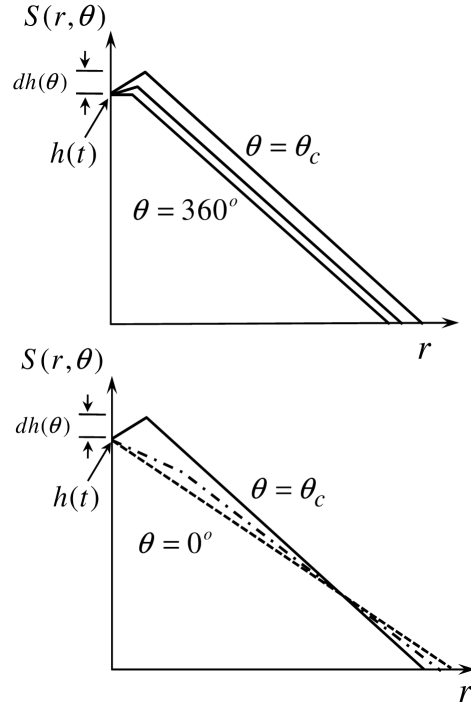
Figure 6: Cuts of the pile side at constant azimuth $\theta$ in the continuous regime. Upper panel: frozen side of the pile, below a crater crest. Lower panel: part where the revolving river passes, and where the surface flow takes place behind it.

The role of this crater on the organization of the flow in revolving rivers seems thus very important. For example, when the incoming sand flux presents too many lateral oscillations or is too wide, the crater and revolving river formation are prevented. Similarly, when the pile has not grown enough to reach a diameter beyond the distance of saltation from the impact point, the crater formation is prevented, and unstable rivers are observed -i.e., beyond the line R1 in Fig. 1. The fact that grains do not bounce too far when they arrive on the pile, i.e. a moderate restitution coefficient, is certainly an important ingredient to allow the crater formation.

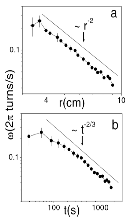
Figure 7: Radius (a) and time (b) dependencies of the frequency of revolution of the rivers (taken from Altshuler2003 ). The points correspond to experimental values.

From this geometry, one can also infer a relationship between the pile radius and the angular velocity, as reported in Altshuler2003 : during a time $dt$, a volume of sand $Fdt$ is deposited over a layer of size $\delta r\tan(\Phi_{0})\omega r^{2}dt/2$, where $\Phi_{0}$ is the respose angle along most of the pile (for azimuth $\theta$ between $\theta_{c}$ and $360^{\circ}$). Consequently, mass conservation of the grains imposes that $\omega=2F/[r^{2}\delta r\tan(\Phi_{0})]$. This power-law dependence of the angular velocity over the pile radius is verified experimentally, as shown in Fig. 7. Since the pile radius increases from flux conservation so that $\pi r(t)^{3}\tan(\Phi_{0})/3=Ft$, i.e. as $r(t)=[3Ft/\pi\tan(\Phi_{0})]^{1/3}$, the angular velocity goes as

$$\omega=(\pi/3)^{2/3}\frac{2F^{1/3}}{\delta r(\tan{\Phi_{0}})^{1/3}}\frac{1}{t^{2/3}}.$$ (1)

This power law decrease of the angular velocity with time is also verified experimentally (Fig. 7).

At a certain critical size of the pile radius $r_{ci}$, the flow becomes intermittent and exhibits avalanches, while still being concentrated along a river. These avalanches extend over a basis $\delta r$ from the pile bottom, comparable to the horizontal extent of layers added by the flowing river in the continuous regime. These avalanches form delta-shaped piles on the side of the main cone, with a slightly carved river penetrating above the apex of the delta (as seen below the pile’s apex, lower panel of Fig. 2) which is “smoothen out” as the river moves on laterally. The slope angle of these delta is lower than the average angle around the pile, with typically a stop angle $\Phi_{1}=33^{\circ}$, as on the flowing part of the continuous regimes, whereas the rest angle for the average slope of the pile is around $\Phi_{0}=36^{\circ}$ –see Fig. 3. The radial extent $l$ of these deltas from the bottom of the pile is set by the geometrical condition $(l+\delta r)\tan(\Phi_{1})=l\tan(\Phi_{0})$ (see Fig. 8), which corresponds to a constant value $l\sim 6cm$, as observed on Fig. 2. Once these deltas are filled to the top, as well as the slightly carved zone above, the river feeding this delta revolves and a new delta is formed by an avalanche developing next to the previous one.

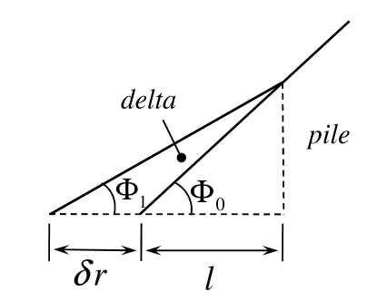
Figure 8: Cuts of the pile near the lower boundary in the intermittent regime.

IV Continuous vs. intermittent regimes: comparison with Hele-Shaw experiments

The transition from continuous to intermittent granular flows have been extensively studied using two basic geometries: the rotating drum Rajchenbach1990 and the Hele-Shaw cell Durian2000 . Typically, the intermittent (or “avalanche”) flow is transformed into continuous flow by increasing the rotation speed of the drum or the input flux, respectively. In the case of the Hele-Shaw cell arrangement, a transition from continuous to intermittent flow (start down and stop up fronts Douady2000 ) takes place when the heap reaches a critical size, even if the input flux and channel width are kept constant. Here we explore such transition in our sand in order to establish an analogy with the sandpile scenario. The cell consisted in a horizontal base and a vertical side-wall, sandwiched between two square glass plates with inner surfaces separated by a distance $w$ in the range from $0.4$ cm to $1.2$ cm. The lengths of the base and the vertical wall were approximately $d\approx 22$ cm. The sand was poured near the vertical wall using a sliding window of width $w$ and variable aperture along the horizontal direction. Although in most of the results we report below the distance between the funnel and the upper side of the heap varied from $10$cm to $1$cm during a typical experiment, we performed some tests keeping the distance fixed at $2$cm, getting similar results. The input volume per unit time, $F$, was calibrated by calculating the volume of sand deposited in the cell in a given time interval.

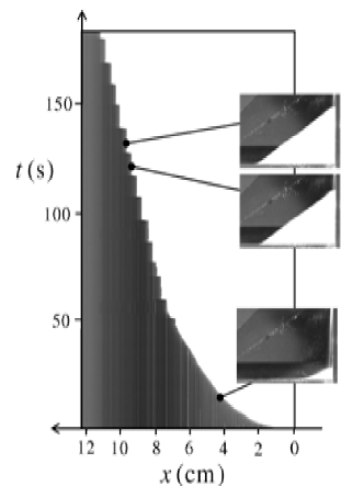
Figure 9: Spatio-temporal diagram of the growing heap. The diagram was made for a sequence of images taken at every $0.1$s to a heap growing in a Hele-Shaw cell with $w=4$ mm and $F=0.125$$cm^{3}/s$. The cuts where taken along an approximately $12$ cm-long horizontal line near the bottom of the cell. As the time goes by, the heap grows continuously, corresponding to a smooth increase of the white area in the diagram. At a critical distance of $7$ cm, avalanches start, and the diagram shows a step-like behavior. The insets on the right contains real pictures of the heap illustrating different moments of the spatio-temporal diagram.

Fig. 9 shows a spatio-temporal diagram of evolution of one heap formed into a cell with $w=4$ mm using an input flux of $0.25$ $cm^{3}/s$. It is based on a digital video acquired with an Optronics Camrecord 600, some of which snapshots are shown as insets. A $15$cm-long horizontal line of pixels was taken $0.5$cm from the bottom of the Hele-Shaw cell every $1/10$ of a second. The spatio-temporal diagram was constructed as a stack of such lines (the darker zones correspond to the air, while the clearer ones correspond to the sand). The position of the row of pixels was taken in such a way, that the interface between dark and clear zones follows the displacements at the lower end of the growing heap. As can be seen at low times, the end of the heap near the bottom of the cell grows smoothly. However, approximately when the horizontal size of the heap reaches a length of $7$cm (see arrow in Fig. 9), the spatio-temporal is no longer smooth, but resembles a ladder: we define in this way the transition between the continuous and the intermittent (or avalanche) regimes. In the latter (well described in references Douady2000 ; Mendes1999 ; Mendes2000 ), sudden avalanches roll downhill (corresponding to the high velocity, almost horizontal segments in the spatio-temporal diagram), and then a front climbs the hill as a new layer of sand is added from bottom to top (corresponding to the zero-velocity, vertical segments in the spatio-temporal diagram). The general shape of this diagram resembles Fig. 2 in Mendes1999 , where the authors use two equations for thick flows proposed in DeGennes1998 to model the heap formation in Hele-Shaw geometry. However, they do not report a continuous-intermittent transition –only the intermittent regime is described. We observe, though, other predictions reported in Mendes1999 , such as the “segmented” profiles of the heaps (see the two upper insets in our Fig. 9) and stratification lines parallel to the free surface of the heaps. However, stratification is only visible in our case after the heap has reached the intermittent regime, i.e., where the model proposed in Mendes1999 fully applies.

By quantifying the critical length, $x_{ci}$, at which the transition between continuous and intermittent flow happens, for different input fluxes, we construct the “phase diagram” presented in Fig. 10. There, the vertical axis represents the input flux as the volume per unit time of sand added to the cell. As the width of the cell is increased, the transition line increases its slope, indicating that, for a given $F$, the intermittent flow is reached for smaller piles. The inset of Figure 10 shows a superposition of the transition line for the case of a Hele-Shaw cell of $w=12mm$ and the two lines $R2$ and $R3$ corresponding to the wide transition to the intermittent regime in the sandpile geometry. The relative position of the lines suggests that the revolving rivers can be taken, to a first approximation, as a $12$-$mm$-wide “revolving Hele-Shaw” cell that performs a revolution around the pile a the same frequency of the rivers Altshuler2003 . Within this picture, the role of the river is just to reduce the dimensionality of the flow in the pile.

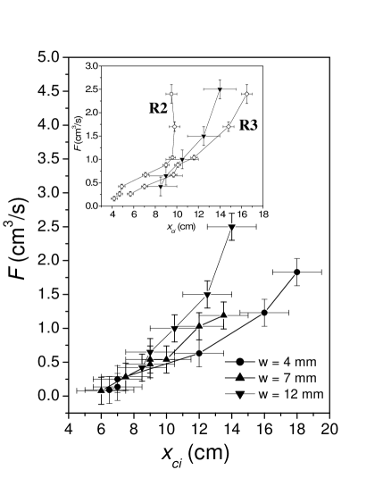
Figure 10: Transition from the continuous to the intermittent regimes in Hele Shaw and revolving rivers configurations. The vertical axis corresponds to input volume of sand per unit time, and the horizontal axis is the length of the base of the heap at the transition. The inset shows a comparison between the line of a $12mm$ width cell and the lines $R1$ and $R2$ taken from Fig. 1.

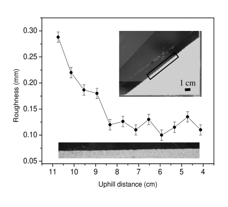
Figure 11: Spontaneous segregation. The graph indicates the decrease in the roughness amplitude of the pile as we move uphill, suggesting segregation of bigger particles near the lower edge of the heap. The roughness amplitude has been measured as the root mean square of the elevation across $12$mm long running windows on the free surface seen in the $7$cm-long picture of the lower inset, corresponding to the boxed region indicated in the upper inset. We define the uphill distance as the distance from a point on the surface to the top of the pile.

The specific mechanism that triggers the transition from the continuous to intermittent regimes as the size of the system grows is still unclear for our sandpiles, and also probably for the Hele-Shaw configuration (we underline that a qualitative explanation is given in Douady2000 for a heap of fixed length). Here we propose an explanation based on segregation. As well known in the case of debris flows in mountains, bigger rocks tend to accumulate in the flow front as it slides down. This is clearly illustrated, for example, in Fig.1.4 of reference Taka1991 . Careful inspection of the free surface of our heaps in the Hele-Shaw configuration also hints at segregation of big grains as we move down the slope, even when our grains are not significantly bi-disperse. In fact, the roughness amplitude of the surface varies from approximately $0.1$mm to $0.3$mm as we move down the hill (see Fig. 11). If one assumes that a slope of bigger grains provides the necessary effective friction to start the growth of a “stop up” front, we speculate that, when the heap grows to a size large enough for the segregation of big grains near the base reaches a certain threshold, the intermittent regime is triggered. In analogy, the increase in the radius of the pile is a necessary condition to reach the intermittent regime in the revolving rivers.

V Conclusions

We have established experimentally the “dynamical phase diagram” of the continuous and intermittent regimes for revolving rivers in sandpiles. One somewhat unexpected feature of the diagram is that stable continuous rivers can only exist below a certain input flux threshold: the intermittent regime is the most robust dynamics in the system. The details of the pile shape and of the movement of grains on its surface indicate that, while most of the downhill flow in the continuous regime takes place within the “river itself”, there is a wide area behind it that contributes with much smaller flow. This fact, however, plays a relevant role in the slow change in the slope as one moves around the pile. We have also improved the kinematic model presented in Altshuler2003 in order to mimic in detail the measured topography of the piles in the continuous regime. The model also allows to estimate the extension of the undulating pattern in the intermittent regime based on other experimental parameters. By performing a series of experiments with Hele-Shaw cells, we conclude that, due to the reduced dimensionality of the granular flow along the rivers, we can describe them as “revolving” Hele-Shaw cells of $12$ mm width –the analogy accounts both for the continuous and the intermittent regimes. Finally, we propose that the segregation of big grains after the pile has reached a critical size is responsible for the appearance of “stop-up” fronts and, consequently, for the transition to the intermittent regime.

- (1) E. Altshuler, O. Ramos, E. Martínez, A. J. Batista-Leyva, A. Rivera, and K. E. Bassler, Phys. Rev. Lett. 91, 014501 (2003).
- (2) X.-Z. Kong, M.-B. Hu, Q.-S. Wu and Y.-H. Wu, Physics Letters A 348, 77 (2006).
- (3) E. Martínez, C. Pérez-Penichet, O. Sotolongo-Costa, O. Ramos, K. J. Måløy, S. Douady and E. Altshuler, Phys.Rev. E. 75, 031303 (2007).
- (4) S. Douady, B. Andreotti and A. Daerr Adv. Complex Systems 4, 509 (2001)
- (5) J. Rachjenbach Phys. Rev.Lett. 65, 2221 (1990)
- (6) P. -A. Lemieux, and D. J. Durian Phys. Rev. Lett. 85, 14273 (2000)
- (7) S. N. Dorogovtsev, and J. F. F. Mendes, Phys. Rev. Lett. 83, 2946 (1999).
- (8) S. N. Dorogovtsev, and J. F. F. Mendes, Phys. Rev. E 61, 2909 (2000).
- (9) Th. Boutreux, E. Raphaël and P. -G. de Gennes Phys. Rev. E 58, 4692 (1998)
- (10) T. Takahashi “Debris Flow”, A. A. Balkema, Rotterdam (1991).