The Kochen-Specker Theorem Revisited
in Quantum Measure Theory
Fay Dowker and Yousef Ghazi-Tabatabai
Blackett Laboratory, Imperial College,
London, SW7 2AZ, U.K.

Abstract

The Kochen-Specker Theorem is widely interpreted to imply that non-contextual hidden variable theories that agree with the predictions of Copenhagen quantum mechanics are impossible. The import of the theorem for a novel observer independent interpretation of quantum mechanics, due to Sorkin, is investigated.

1 Introduction

Though quantum mechanics is extremely successful in making experimental predictions it has proved unusually difficult to understand or interpret, to the extent that the interpretation of quantum mechanics has become a field of research in itself. While an instrumentalist approach evades these problems in the context of open systems with external observers to hand, in the application of quantum mechanics to closed systems, as called for by the search for a quantum theory of gravity, a notion of objective reality becomes all the more necessary. The spacetime nature of reality as revealed by Special and General Relativity also puts pressure on the text-book version of quantum theory in which a vector in a Hilbert space plays a central role.

As argued by Hartle [1] the development of the Sum Over Histories (SOH) by Dirac [2] and Feynman marked the beginnings of a new framework for quantum mechanics in which a more observer independent, and fully spacetime view of reality could be pursued. Indeed Feynman’s original paper is entitled “Space-time approach to non-relativistic quantum mechanics” [3] and in his Nobel Lecture he described how “[he] was becoming used to a physical point of view different from the more customary point of view. […] The behavior of nature is determined by saying her whole spacetime path has a certain character.” [4]

In a SOH framework, the structure of a quantum theory is more akin to a classical stochastic theory such as Brownian motion than any classical Hamiltonian theory, the kinematics consisting of a space of histories or “formal trajectories” of the system and the dynamics being a quantal generalisation of a probability measure on that space. Due to the presence of interference between histories, however, the quantal measure cannot be interpreted as a probability distribution and the challenge has been to furnish the SOH with an interpretation that would make it an observer independent theory consistent with experimental observation.

To date, the most widely studied attempt to interpret the SOH is the “consistent histories” or “decoherent histories” approach and in its SOH formulation (as opposed to its “projection operator” form) has been championed primarily by Hartle [5, 6]. In this approach, the interpretational difficulty that interference causes is dealt with by imposing the rule that only partitions of the space of histories (coarse grainings) such that there is no residual interference between elements of the partition are allowed to be considered. The quantal measure, when restricted to the elements of such a partition, behaves like a classical probability measure and this is the basis for the decoherent histories interpretation.

Sorkin has proposed an alternative approach to finding an interpretation of the SOH [7, 8] starting from an analysis of the interpretational structure of classical stochastic theories. He identified three basic structures in such a classical theory: a Boolean algebra, A, of “questions” that can be asked about the system (or “propositions”, “predicates” or “events”), a space of “answers” (or “truth values”) which classically is $\mathbb{Z}_{2}=\{0,1\}=\{false,true\}=\{no,yes\}$, and the space of allowed “answering maps” $\phi:{\hbox{\german A}}\rightarrow\mathbb{Z}_{2}$ which classically is the space of non-zero homomorphisms. Each answering map, or co-event, $\phi$, corresponds to a possible reality and its being a homomorphism is equivalent to the use of Boolean (ordinary) logic to reason about classical reality.

To generalise this structure to the quantal case, Sorkin proposes to keep both the “event algebra” A and the truth values, $\mathbb{Z}_{2}$ as they are but relax the condition that the answering map/co-event $\phi$ must be a homomorphism. Thus, the general framework can be described as one that embraces “Anhomomorphic Logic”.

The freedom to incorporate Anhomomorphic Logic enables the identification of co-events $\phi$ as potential objective realities in a quantum theory. The framework is therefore challenged to provide an account of the standard counter-examples to the classical realist approach, in particular the celebrated Kochen-Specker theorem [9]. This paper will go some way to showing that this is indeed possible in a specific proposed scheme which we will call, after Sorkin, the Multiplicative Scheme.

First we outline Quantum Measure Theory and describe the Multiplicative Scheme. We then review the Peres version of the Kochen-Specker theorem, and recast it in the language of quantum measure theory. We show that although there is no homomorphic co-event for the Peres-Kochen-Specker event algebra there is a multiplicative co-event. We then show that this quantum measure theory version of the Peres setup can be concretely realised as a Peres-Kochen-Specker gedankenexperiment in terms of the spacetime paths of a spin 1 particle though a sequence of beam splitters and recombiners. We sketch an account of this gedankenexperiment in the Multiplicative Scheme.

2 Quantum Measure Theory

The kinematics of a classical stochastic theory, such as a random walk, is specified by a space, $\Omega$, of possible histories or formal trajectories. For simplicity we will assume here and in the quantal case that all spaces are finite. Then the event algebra, A, referred to in the introduction is the Boolean algebra of all subsets of $\Omega$.

The dynamics of a classical stochastic theory is encoded in a measure, $|\cdot|$ such that

$$|\cdot| :\ \ {\hbox{\german A}}\rightarrow\mathbb{R}$$

$$|A| \geq 0\ \ \forall A\in{\hbox{\german A}}\ \ \text{(Positivity)}$$

$$|A\sqcup B| =|A|+|B|\ \ \forall A,B\in{\hbox{\german A}}\,,\ \text{where}\ A,B\ \text{disjoint}\ \ \text{(Kolmogorov Sum rule)}$$

$$|\Omega| =1\ \ \text{(Normalisation)}\,.$$ (1)

Elements of A will be referred to as events and each event corresponds to a question that can be asked about the system.

One can think of a possible reality as giving a set of true/false answers to every question that can be asked, in other words it is a map, $\phi$, from A to $\mathbb{Z}_{2}$, a co-event (so called because it takes events to numbers). The set of all such maps will be denoted ${\hbox{\german A}}^{*}$. Now a classical stochastic theory distinguishes exactly one of the fine grained histories (say $\gamma\in\Omega$) as the ‘real history’. A question $A\in{\hbox{\german A}}$ is also a subset of $\Omega$, and is ‘true’ if and only if it contains the real history $\gamma$. We can then express this state of affairs as a co-event $\gamma^{*}\in{\hbox{\german A}}^{*}$ mapping to $1$ (true) exactly those elements of A that contain the real history $\gamma$:

$$* :\ \ \Omega\rightarrow{\hbox{\german A}}^{*}$$

$$* :\ \ \gamma\mapsto\gamma^{*}\,,$$

where

$$\gamma^{*}(A)= \,\left\{\begin{array}[]{cc}1&\text{if}\ \gamma\in A\\ 0&\text{otherwise}\end{array}\right.$$

The “mind flip” from formal trajectory, $\gamma$, to co-event, $\gamma^{*}$, as representing reality turns out to be fruitful in moving on to the quantum case. We will refer to co-events such as $\gamma^{*}$, where $\gamma$ is an element of $\Omega$, as classical co-events.

A is a boolean algebra with the operations symmetric difference as addition and intersection as multiplication. $\mathbb{Z}_{2}$ is also a Boolean algebra and the classical co-events are precisely the homomorphisms from A to $\mathbb{Z}_{2}$.

Lemma 1.

Given a finite sample space $\Omega$ and an associated event algebra ${\hbox{\german A}}=2^{\Omega}$

$$\{\gamma^{*}|\gamma\in\Omega\}=Hom({\hbox{\german A}},\mathbb{Z}_{2})$$ (2)

where the zero map is excluded from $Hom({\hbox{\german A}},\mathbb{Z}_{2})$.

Understanding the role of the measure $|\cdot|$ is controversial, even in a classical stochastic theory where it is tantamount to understanding the interpretation of probability. Sorkin, following Geroch [10] among others, has adopted the view that the predictive, scientific content of a stochastic theory (classical or quantal) is exhausted by the requirement of “preclusion” whereby an event of zero measure will be valued “false” in reality. In other words, allowed co-events, $\gamma^{*}$, are “preclusive”:

$$|A|=0\Rightarrow\gamma^{*}(A)=0$$ (3)

Thus if an event $A\in{\hbox{\german A}}$ is precluded by the measure, $|A|=0$, then any co-eve nt that is an ‘admissible’ description of the system is of the form $\gamma^{*}$ and must obey $\gamma^{*}(A)=0$. This is equivalent to the condition that the real history, $\gamma$, cannot be an element of $A$. This is straightforward and uncontroversial but it is exactly this condition that will cause problems with a classical interpretation of quantum mechanics, as we shall see.

The structure of a quantal measure theory [7, 8] is the same as the classical one in many respects and we will use the same notation: a space, $\Omega$ of formal trajectories and the corresponding Boolean algebra of events, A, give the kinematics of the theory. The dynamics is encoded in a measure which is again a non-negative, normalised, real function, $|\cdot|$, on the event algebra. However, the Kolmogorov Sum Rule is replaced by its quantal analogue:

$$|A\sqcup B\sqcup C|=|A\sqcup B|+|B\sqcup C|+|A\sqcup C|-|A|-|B|-|C|\ \ \forall A,B,C\in{\hbox{\german A}},\ \text{disjoint}\,$$ (4)

which is just one of a whole hierarchy of conditions that define higher level “generalised measure theories” [12]. This replacement leads to important differences with the classical theory, in particular, in contrast to a probability measure, due to interference a measure zero set can now contain sets that have positive measure. More generally, $A\subset B$ no longer implies $|A|\leq|B|$.

An alternative (more or less equivalent [12]) set of axioms for the dynamical content of a quantal theory is based on the so-called “decoherence functional”, $D:{\hbox{\german A}}\times{\hbox{\german A}}\rightarrow\mathbb{C}$ which satisfies the conditions [5, 6]:

(i) Hermiticity: $D(X;Y)=D(Y;X)^{*}$ ,  $\forall X,Y\in{\hbox{\german A}}$;

(ii) Additivity: $D(X\sqcup Y;Z)=D(X;Z)+D(Y;Z)$ , $\forall X,Y,Z\in{\hbox{\german A}}$ with $X$ and $Y$ disjoint;

(iii) Positivity: $D(X;X)\geq 0$ ,  $\forall X\in{\hbox{\german A}}$;

(iv) Normalisation: $D(\Omega;\Omega)=1$ .

The quantal measure is given by a decoherence functional via

$$|X|=D(X;X)\,.$$ (5)

and it satisfies the condition in equation 4. All known quantum theories have their dynamics encoded as a decoherence functional, from which the quantal measure is defined as above. To see how the decoherence functional is defined for ordinary non-relativistic particle quantum mechanics see for example [6, 13].

Reality is to be identified with a co-event, $\phi$, an element of ${\hbox{\german A}}^{*}$ as before but in the quantal case, there are obstructions to demanding that the co-event be a homomorphism. The celebrated Kochen-Specker theorem is one such obstruction and we will explore this explicitly in the next section.

2.1 The Multiplicative Scheme

A homomorphic co-event respects both the sum (“linearity”) and product (“multiplicativity”) structure of the algebra A:

$$\phi(A+B)= \,\phi(A)+\phi(B)\ \ \text{and}$$

$$\phi(AB)= \,\phi(A)\phi(B)\ \ \forall A,B\in{\hbox{\german A}}\,,$$

where $A+B=(A\setminus B)\cup(B\setminus A)$ is symmetric difference and $AB=A\cap B$ (recall that $A$ and $B$ are identified with subsets of $\Omega$). The Multiplicative Scheme [8] for Anhomormorphic Logic can be motivated from several directions. Algebraically, it can be defined by requiring that real co-events preserve multiplicativity,

$$\phi(AB)=\phi(A)\phi(B)\ \forall A,B\in{\hbox{\german A}}\;,$$

while the linearity condition is dropped. The two trivial co-events $\phi=1$ and $\phi=0$ are excluded by fiat in the scheme.

Lemma 2.

If $\phi$ is multiplicative then the set of events $\phi^{-1}(1)$,

$$\phi^{-1}(1)=\{A\in{\hbox{\german A}}|\phi(A)=1\}\,,$$

is a filter.

Proof.

Let $\phi$ be a multiplicative co-event and let $A\in\phi^{-1}(1)$. If $A\subset B$ then $AB=A$ and therefore $1=\phi(A)=\phi(AB)=\phi(A)\phi(B)=\phi(B)$. Which means that $B\in\phi^{-1}(1)$. Further, if $A,~{}B\in\phi^{-1}(1)$ then $\phi(AB)=\phi(A)\phi(B)=1$, so $A\cap B\in\phi^{-1}(1)$, thus $\phi^{-1}(1)$ is a filter. ∎

Note that this proof holds for infinite $\Omega$ also. However, every finite filter is a principal filter, so if $\Omega$ is finite (as we are assuming unless otherwise stated) then $\phi^{-1}(1)$ is a principal filter. To see this first note that because $\Omega$ and thus A are finite, $\phi^{-1}(1)$ must contain a minimal element (minimal under set inclusion) $\Phi$. If $\Xi$ is also a minimal element of the filter then $\Phi\cap\Xi$ is in the filter, is contained in both $\Phi$ and $\Xi$ and therefore must be equal to both. Therefore $\Xi=\Phi$ and $\Phi$ is the unique minimal element and the principal element of $\phi^{-1}(1)$. Note that $\Phi$ is not empty since otherwise $\phi=1$ which is excluded. In the terminology of reference [8], $\Phi$ can also be called the support of the multiplicative co-event $\phi$.

It is convenient to identify a multiplicative co-event $\phi$ with its support, i.e. the principal element $\Phi$ of the associated filter. We define a map

$$* :\ \ {\hbox{\german A}}\rightarrow{\hbox{\german A}}^{*}$$

$$* :\ \ A\mapsto A^{*}\,,$$

where

$$A^{*}(B)= \ \left\{\begin{array}[]{cc}1&{\text{if}~{}A\subset B}\\ 0&{\text{otherwise}}\end{array}\right.$$

Note that, using this notation, $\{\gamma\}^{*}=\gamma^{*}$. The map $*$ is clearly 1-1 and its image is the set of all multiplicative co-events (for finite $\Omega$). The inverse of $*$ is the map that takes a multiplicative co-event, $\phi$, to the principle element, $\Phi$, of the associated filter.

The natural order on filters furnishes us with a simple notion of minimality or primitivity. We say that a preclusive multiplicative co-event $\phi$ is minimal or primitive if the associated filter $\phi^{-1}(1)$ is maximal among the filters corresponding to preclusive multiplicative co-events. Primitivity can be thought of as a condition of “maximal detail” or “finest graining” consistent with preclusion (“Nature abhors imprecision”) and we adopt this as a further condition on real co-events in the Scheme. This allows us to deduce classical logic when the measure happens to be classical:

Lemma 3.

If $\phi$ is a primitive preclusive multiplicative co-event and the measure $|\cdot|$ is classical, then $\phi$ is a homomorphism.

Proof.

Consider $\Phi\in{\hbox{\german A}}$ such that $\phi=\Phi^{*}$. The Kolmogorov sum rule implies that the union, $Z$, of measure zero sets in A is itself of measure zero, so the preclusivity of $\phi$ implies $\Phi\not\subset Z$. Thus $\exists\gamma\in\Phi\setminus Z$ such that $\gamma$ is not an element of any measure zero set. This means that $\gamma^{*}$ is preclusive, but then the minimality of $\phi$ means that $\Phi=\{\gamma\}$ and so $\phi=\gamma^{*}$, a homomorphism. ∎

All non-zero multiplicative co-events are unital, in other words $\phi(\Omega)=1$ when $\phi$ is multiplicative. So a multiplicative co-event answers the question “Does anything at all happen?” with “Yes”! A nonzero preclusive multiplicative co-event always exists, indeed $\Omega^{*}$ is always a preclusive multiplicative co-event. Moreover, if $A$ is an event with nonzero measure that is not contained in any event with zero measure then $A^{*}$ is preclusive. Therefore there exists at least one primitive preclusive multiplicative co-event in which $A$ happens.

3 The Kochen-Specker Theorem

The Kochen-Specker (KS) theorem [9] is often cited as a key obstacle to a realist interpretation of quantum mechanics. We will situate the KS theorem in the framework of event algebras and co-events described above.

We will use Peres’ proof of the Kochen-Specker Theorem [14] and rely on his 33-ray construction.

Peres defines 33 rays in $\mathbb{R}^{3}$ from which 16 orthogonal bases can be formed. Peres defines the rays as being the 33 for which the squares of the direction cosines are one of the combinations:

$$0+0+1=0+1/2+1/2=0+1/3+2/3=1/4+1/4+1/2\,.$$

Figure 1 (taken with permission from [15]) illustrates the points where the rays intersect a unit cube centred on the origin.

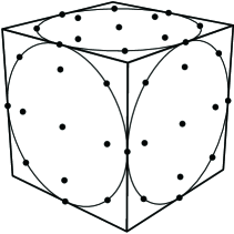
Figure 1: The $\pm 33$ directions are defined by the lines joining the center of the cube to the $\pm 6$ mid–points of the edges and the $\pm 3$ sets of 9 points of the $3\times 3$ square arrays shown inscribed in the incircles of its faces

To describe the rays, Peres employs a shorthand notation that we will find useful, writing $\overline{x}=-x$ we define

$$\overline{x}yz=\alpha\left(\begin{array}[]{c}-x\\ y\\ z\end{array}\right)\in\mathbb{R}^{3}$$

where $\overline{xyz}=xyz$ as we are dealing with rays rather than vectors. We will call this set of rays the Peres Set, $PS$, and sometimes it will be convenient to refer to them as labelled from 1 to 33: $PS=\{u_{i}|i=1,2,\dots 33\}$ (in some fixed but arbitrary order).

In what follows it will be important to understand the structure & the symmetries of $PS$. Examining the magnitude of the angle between each ray and its nearest neighbour, we find that the rays can be divided into four types:

Type I: $001,010,100$

Type II: $011,01\overline{1},101,10\overline{1},110,1\overline{1}0$

Type III: $012,0\overline{1}2,021,02\overline{1},102,\overline{1}02,201,20\overline{1},120,\overline{1}20,210,2\overline{1}0$

Type IV: $112,\overline{1}12,1\overline{1}2,\overline{1}\overline{1}2,121,12\overline{1},\overline{1}21,\overline{1}2\overline{1},211,21\overline{1},2\overline{1}1,2\overline{1}\overline{1}$

Table 1: The Peres rays divide into 4 Types.

With reference to figure 1, Type I corresponds to the midpoints of faces of the cube, Type II to the midpoints of edges, Type III to the remaining points in the interior of the incircles of the faces and Type IV to the remaining points on the incircles of the faces. It can be seen that each symmetry of the projective cube induces a permutation of $PS$. The symmetry group of the projective cube, $H$, is of order 24 and is generated by rotations by $\pi/2$ around co-ordinate axes and reflections in co-ordinate planes. Since the ray types are defined in terms of angles, the induced permutations on the elements of $PS$ will preserve the type of each ray, i.e. the permutation reduces to permutations on the four subsets of same-type rays. By inspection, $H$ is transitive on each type: this means that for any two rays $u$, $v$ of the same type $\exists$ $g\in H$ such that $v=g(u)$.

In the Peres version of the Kochen-Specker theorem, this set of 33 rays is mapped in the obvious way into a set of rays in a 3 dimensional Hilbert space, where two rays are orthogonal in the Peres set if and only if they are mapped to orthogonal rays in Hilbert space. We will therefore talk about the Peres rays both as rays in real 3-D space and in Hilbert space. To each orthogonal basis of rays, $\{u_{i},u_{j},u_{k}\}$, in Hilbert space can be associated an observable with three distinct outcomes, each outcome corresponding to one of the rays in the basis (the eigenvector of the outcome/eigenvalue). If that observable is measured, one of the three outcomes will be obtained and the quantum state collapses onto exactly one of the three basis rays, which corresponds to the outcome. If it is assumed that the result of the measurement of the observable exists within the system before or independent of the measurement being taken – a non-contextual hidden variable – then we would conclude that one of the basis rays corresponds to the actual value of the observable being measured, and is labelled “true”, and the other two (using classical logic) are labelled “false”. We follow Peres in considering the the “true” ray to be coloured green whereas the other two are coloured red.

Assuming that an experimenter can freely choose to measure any of the observables associated to the 16 orthogonal bases in $PS$, if we assume that the result of the measurement actually done is encoded in the system beforehand, then the results of all potential measurements must be encoded in the system. Thus, all of the rays in $PS$ will be coloured. We call a map

$$\gamma:PS\rightarrow\{green,red\}$$

a colouring. We call $\gamma$ a consistent colouring if it colours exactly one ray green out of every basis in $PS$ (we assume henceforth that “basis” implies “orthogonal basis”) and does not colour any pair of orthogonal rays both green. Note there are some orthogonal pairs in $PS$ that are not contained in a basis in $PS$.

Basis	Basis Rays	Other Orthogonal Rays
$B_{1}$	$\textbf{001}~{}100~{}010$	$110~{}1\overline{1}0$
$B_{2}$	$\textbf{101}~{}\overline{1}01~{}\textit{010}$
$B_{3}$	$\textbf{011}~{}0\overline{1}1~{}\textit{100}$
$B_{4}$	$\textbf{1$\overline{\textbf{1}}$2}~{}\overline{1}12~{}\textit{110}$	$20\overline{1}~{}021$
$B_{5}$	102 20$\overline{\textit{1}}$ 010	$2\overline{11}$
$B_{6}$	211 0$\overline{\textit{1}}$1 2$\overline{\textit{11}}$	$\overline{1}02$
$B_{7}$	201 010 $\overline{\textit{1}}$02	$\overline{11}2$
$B_{8}$	112 1$\overline{\textit{1}}$0 $\overline{\textit{11}}$2	$02\overline{1}$
$B_{9}$	012 100 02$\overline{\textit{1}}$	$\overline{1}2\overline{1}$
$B_{10}$	121 $\overline{\textit{1}}$01 $\overline{\textit{1}}$2$\overline{\textit{1}}$	$0\overline{1}2$
$B_{11}$	100 021 0$\overline{\textit{1}}$2

Table 2: Peres’ Proof of the Kochen-Specker Theorem

Theorem 1.

Peres-Kochen-Specker [14]
There is no consistent colouring of $PS$

Proof.

The proof is based on table 2. First assume there is a consistent colouring of $PS$. This colouring must be consistent on all bases in $PS$, in particular it must be consistent on the four bases $B_{1},~{}B_{2},~{}B_{3},~{}B_{4}$. These bases intersect, and there are $24$ consistent colourings, of the $10$ rays in $\bigcup_{i}B_{i}$. It is easy to see [14] that these 24 colourings are related to each other by the 24 symmetries of the projective cube. Consider a single fiducial colouring, $\gamma_{P}$ of the four bases, $B_{1},~{}B_{2},~{}B_{3},~{}B_{4}$, as defined in table 2, which colours green the first ray in each basis except for $B_{11}$ (highlighted in bold in the table). We then work down the table basis by basis starting at $B_{5}$ to try to extend $\gamma_{P}$ to a consistent colouring of $PS$. For each basis $B_{i}$, $i>4$, in turn we find that two of the basis elements (italicised) have already been coloured red, and so in each case the choice of basis ray to colour green is forced by consistency. This continues until we reach basis $B_{11}$, which by then has all three basis rays coloured red, meaning that $\gamma_{P}$ cannot be extended to a consistent colouring of the whole Peres Set. Now, as noted above every consistent colouring $\gamma_{Q}$ of $B_{1},~{}B_{2},~{}B_{3},~{}B_{4}$ is related to $\gamma_{P}$ by a symmetry, thus $\gamma_{Q}=g(\gamma_{P})$ for some $g\in H$. Thus if we were to attempt to extend $\gamma_{Q}$ to a consistent colouring of the whole Peres Set we would find the same contradiction on $g(B_{11})$. Thus no consistent colouring of $B_{1},~{}B_{2},~{}B_{3},~{}B_{4}$ can be extended to $PS$, therefore there is no consistent colouring of the Peres Set. ∎

3.1 Event algebras and co-events

Let us now restate the theorem in terms of event algebras and co-events. Let the space $\Omega$ be the set of all (green/red) colourings, $\gamma$ of the Peres set $PS$. The event algebra is the Boolean algebra of subsets of $\Omega$ as before. Given a subset $S$ of the Peres Set we write:

$$R_{S}= \{\gamma\in\Omega|~{}\gamma(u_{i})=red~{}\forall u_{i}\in S\}$$ (6)

$$G_{S}= \{\gamma\in\Omega|~{}\gamma(u_{i})=green~{}\forall u_{i}\in S\}$$ (7)

Now the Kochen-Specker-Peres result depends crucially upon disallowing, or precluding, non-consistent colourings. Thus in measure theory language, we wish to consider the sets corresponding to these failures in consistency to have measure zero (though we will not explicitly construct a measure until section 5). These inconsistencies arise in two ways, an orthogonal pair of rays being coloured green or an orthogonal basis of rays being coloured red, thus we treat the following two types of set as if they are of measure zero:

$$R_{B} B~{}\text{an orthogonal basis}$$ (8)

$$G_{P} P~{}\text{an orthogonal pair}$$ (9)

We will call these the Peres-Kochen-Specker (PKS) events, or PKS sets. Note that the Peres Set includes orthogonal pairs that are not subsets of orthogonal bases.

Now (as already implicitly assumed in the proof of Theorem 1) every symmetry $g\in H$ of the projective cube induces an action on $\Omega$ and thus on A, via its action on $PS$. We will also denote this action by $g\in H$, so that $g\cdot\gamma(u_{i})=\gamma(g\cdot u_{i})$ and $g(A)=\{g(\gamma)|\gamma\in A\}$. Crucially, note that the PKS sets are permuted by the symmetries in $H$, via $g(G_{P})=G_{g(P)}$ and $g(R_{B})=R_{g(B)}$.

In the language of measures and co-events, the Peres-Kochen-Specker result can be stated:

Lemma 4.

Let $|\cdot|$ be a measure on the space $\Omega$ of colourings of $PS$ that is zero valued on the PKS sets. Then there is no preclusive classical co-event for this system.

Proof.

By Theorem 1, every element of $\Omega$ is inconsistent on at least one basis or pair and therefore lies in at least one PKS set. Consider $\gamma^{*}$, a classical co-event. $\gamma$ lies in at least one PKS set and therefore $\gamma^{*}$ is not preclusive. ∎

4 Kochen-Specker in the Multiplicative Scheme

Can multiplicative co-events succeed where the classical scheme fails in providing a satisfactory account of the PKS system? In particular, can we avoid non-existence results such as lemma 4? Trivially, yes, since $\Omega^{*}$ is always a preclusive multiplicative co-event regardless of the measure, because we have a priori imposed $|\Omega|\neq 0$ (equation 1). However this is neither interesting nor useful, since the only event mapped to $1$ by $\Omega^{*}$ is $\Omega$ itself. In other words the only question answered in the affirmative is, “Does anything occur?”.

$\Omega^{*}$ is too coarse grained to be useful and, indeed, the axioms of the Scheme are that only the finest grained or primitive preclusive co-events are potential realities. So we need to examine co-events that are minimal among the multiplicative co-events mapping all the PKS sets and their disjoint unions to zero.

Every multiplicative co-event is a principal filter, in particular every multiplicative co-event is of the form $A^{*}$ for some $A\in{\hbox{\german A}}$ where

$$A^{*}(B)=\left\{\begin{array}[]{cc}1&A\subset B\\ 0&otherwise\end{array}\right.$$

$\forall~{}B\in{\hbox{\german A}}$. Hence a multiplicative co-event, $A^{*}$, that values the PKS sets and their disjoint unions zero, has as its support $A$ that is not contained in any PKS set or any disjoint union of PKS sets.

The Peres-Kochen-Specker theorem says that every $\gamma\in\Omega$ is an element of at least one PKS set. Some elements of $\Omega$, however, lie in exactly one PKS set and so are good places to start building a primitive co-event. If we can find two elements $\gamma,\gamma^{\prime}\in\Omega$ that each lie in exactly one PKS set, different for each and not disjoint, then the set containing $\gamma$ and $\gamma^{\prime}$ will be not contained in any PKS set or disjoint union of PKS sets.

Looking at the proof of Theorem 1, we see there is a unique was to extend $\gamma_{P}$ from the four bases $B_{1}$, $B_{2}$, $B_{3}$, $B_{4}$ to the whole of $PS$ so that it is consistent on all bases and pairs of rays except basis $B_{11}$. We will henceforth refer to this extension as the Peres colouring and use the same notation $\gamma_{P}$ for it. The Peres colouring lies in exactly one PKS set, $R_{B_{11}}$ (see equation 8). $\gamma_{P}$ is given in table 3.

We can obtain another such colouring $\gamma_{P}^{\prime}$ by acting on $\gamma_{P}$ by one of the symmetries of the projective cube: let us choose the reflection that exchanges the $x$ and $y$ axis. The colouring $\gamma_{P}^{\prime}$ is then obtained from $\gamma_{P}$ by permuting the rays by the action of swapping the first and second labels (in the Peres notation we have used where a ray is labelled by the components, e.g. $001$). $\gamma_{P}^{\prime}$ is also given in table 3. By symmetry, $\gamma_{P}^{\prime}$ is also contained in exactly one PKS set, $R_{B_{7}}$.

The PKS sets $R_{B_{7}}$ and $R_{B_{11}}$ are not disjoint because they share, for example, the colouring which is red on all rays.

Therefore, the multiplicative co-event $\phi_{M}\equiv\{\gamma_{P},\gamma_{P}^{\prime}\}^{*}$ will value all PKS sets and disjoint unions of PKS sets zero and it is minimal among multiplicative co-events that do so because neither of the atomic co-events will do so.

4.1 Events that can happen

Suppose an event, $X$, has non-zero measure and is not contained in an event of zero measure. Then that event is the support of a preclusive, multiplicative co-event, $X^{*}$ that values $X$ as $1$. So we are guaranteed that a primitive preclusive co-event that values $X$ as $1$ exists: that event could happen.

Let us assume that there is a quantum measure on $\Omega$ the set of colourings of the Peres rays in which the only sets of measure zero are the PKS sets and their disjoint unions. Then for any Peres ray $u_{k}$, the two events “$u_{k}$ is coloured green” and “$u_{k}$ is coloured red” both have non-zero measure and are not contained in any PKS set and the following constructions produce concrete examples of primitive preclusive co-events in which these events happen.

Let $u_{k}$ be one of the Peres rays and let $G_{k}\in{\hbox{\german A}}$ be the event that $u_{k}$ is coloured green and $R_{k}\in{\hbox{\german A}}$ be the event that $u_{k}$ is coloured red. such that $\phi^{r}_{Mk}(R_{k})=1$ and $\phi^{g}_{Mk}(G_{k})=1$.

We start with $\phi_{M}$ (as defined above) which maps the PKS sets to zero and is minimal among the multiplicative events that do so. Every symmetry of the cube induces an action on the space of multiplicative co-events by simultaneously acting on all colourings in the support of a co-event. Moreover, since the PKS sets are mapped to each other under the symmetries of the cube, any co-event which values the PKS sets zero will be mapped, under a symmetry, to one which also values the PKS sets zero.

Table 3 shows the valuation of $\phi_{M}$ on the colourings of all the rays in PS. We note that among the rays, $u_{i}$ for which $\phi_{M}(G_{i})=1$ is at least one of each type (see list 1). So given a ray $u_{k}$, we can find one, $u_{k^{\prime}}$ of the same type for which $\phi_{M}(G_{k^{\prime}})=1$. There is a symmetry of the cube which sends $u_{k^{\prime}}$ to $u_{k}$. Acting with that symmetry on $\phi_{M}$ produces a co-event, call it $\phi_{Mk}^{g}$, with the required properties.

Similarly, among the rays $u_{i}$ for which $\phi_{M}(R_{i})=1$ are at least one of each type so we can find one, $u_{k^{\prime\prime}}$, which of the same type as $u_{k}$. Acting on $\phi_{M}$ with a symmetry that takes $u_{k^{\prime\prime}}$ to $u_{k}$ produces a co-event, $\phi_{Mk}^{r}$, with the required properties.

$u_{i}$		$\gamma_{P}$	$\gamma_{P}^{\prime}$	$\phi_{M}(G_{i})$	$\phi_{M}(R_{i})$
$001$		g	g	1	0
$010$		r	r	0	1
$100$		r	r	0	1
$011$		g	g	1	0
$01\overline{1}$		r	r	0	1
$101$		g	g	1	0
$10\overline{1}$		r	r	0	1
$110$		r	r	0	1
$1\overline{1}0$		r	r	0	1
$012$		g	g	1	0
$0\overline{1}2$		r	r	0	1
$021$		r	g	0	0
$02\overline{1}$		r	r	0	1
$102$		g	g	1	0
$\overline{1}02$		r	r	0	1
$201$		g	r	0	0
$20\overline{1}$		r	r	0	1
$120$		r	r	0	1
$\overline{1}20$		r	r	0	1
$210$		r	r	0	1
$2\overline{1}0$		r	r	0	1
$112$		g	g	1	1
$\overline{1}12$		r	g	0	0
$1\overline{1}2$		g	r	0	0
$\overline{11}2$		r	r	0	1
$121$		g	g	1	0
$12\overline{1}$		r	r	0	1
$\overline{1}21$		r	r	0	1
$\overline{1}2\overline{1}$		r	r	0	1
$211$		g	g	1	0
$21\overline{1}$		r	r	0	1
$2\overline{1}1$		r	r	0	1
$2\overline{11}$		r	r	0	1

Table 3: A minimal unital multiplicative co-event sending the PKS sets to zero

4.2 A closer look at $\phi_{M}$

Looking at the table, we see that for most of the rays we have $\phi(G_{i})+\phi(R_{i})=1$ which is the familiar situation in classical logic, for example if it is false that $u_{i}$ is green then it is true that it is red. However, there are some rays, $021,201,\overline{1}12$ and $1\overline{1}2$, for which both $\phi(G_{i})=0$ and $\phi(R_{i})=0$. Note that there are no rays for which $\phi(G_{i})=1$ and $\phi(R_{i})=1$. This is not a coincidence: $\phi(X)\phi(1+X)=\phi(0)=0$ ($\phi(0)=1$ would imply $\phi=1$ since every event contains the empty event) and so an event and its complement cannot both be valued true. An event and its complement can both be valued false as we see here and indeed this is the epitome of the nonclassical logic that the scheme tolerates.

This violation of classical rules of inference may at the first encounter seem unpalatable. However, it is the way in which a genuine coarse graining is expressed at the level of logical inference. One way to think of the multiplicative co-event is that reality corresponds to the support of the co-event and only common properties of all the formal trajectories in the support are real properties: if the support is contained in an event then that event happens. In this way, both an event and its complement – e.g. ray $u_{i}$ is green and ray $u_{i}$ is red – can be valued false if the support of the co-event intersects them both.

The step in accepting the logic of multiplicative co-events may not be so great, therefore, but we have to deal with the question of whether such a co-event as $\phi_{M}$ represents a contradiction with experimental facts. Can not we check to see whether $u_{i}$ is red and whether it is green and if we always find it is one or the other (and never neither) then wouldn’t that contradict the proposal that $\phi_{M}$ is a possible reality? We will address this question in the context of the concrete experimental setup of the next section.

5 Expressing the Peres-Kochen-Specker setup in terms of Spacetime Paths

Thus far our analysis has been completely abstract and we now seek to embed our mathematical Peres-Kochen-Specker system into a more physical, even perhaps experimentally realisable, framework. To this end we imagine a sequence of Stern-Gerlach apparatus to translate each colouring in $\Omega$ into a spacetime history. We will construct a quantum measure on the corresponding event algebra in which the translations of the Kochen-Specker sets have measure zero, though further ‘accidental’ measure zero sets are introduced as will be discussed.

5.1 The Stern-Gerlach Apparatus

The Stern-Gerlach apparatus allows spin to be expressed in terms of paths in spacetime. In the original experiment (1922) a beam of spin $1/2$ silver atoms was sent through an inhomogeneous magnetic field, splitting the beam into two components according to the spin of the particles.

In our gedankenversion of the Stern-Gerlach experiment we imagine spin 1 particles sent though a parallel, static, inhomogeneous magnetic field B. By parallel we mean that vectors $\textbf{B}(x,t)$ are parallel in the vicinity of the particle beam. By static we mean that $\textbf{B}(x,t)$ is independent of t. We shall also assume that the gradient of the B field is constant close to the beam. Now a particle with spin S will have an effective magnetic moment in the $-\textbf{S}$ direction. Hence the particle will experience a force:

$${\bf F}\propto\nabla(\textbf{S}\cdot\textbf{B})$$

The force is proportional to the component of the spin in the direction of the magnetic field and so the beam will split into three branches, corresponding to the three possible spin states. So for a single particle a measurement ascertaining which branch holds the particle constitutes a measurement of the component of the spin in the direction of the magnetic field. Note that we can thus measure the spin in any direction other than along the path of the beam. However, if such a measurement is not taken, the three branches can be coherently recombined by application of the field $-\textbf{B}$ (see figure 2).

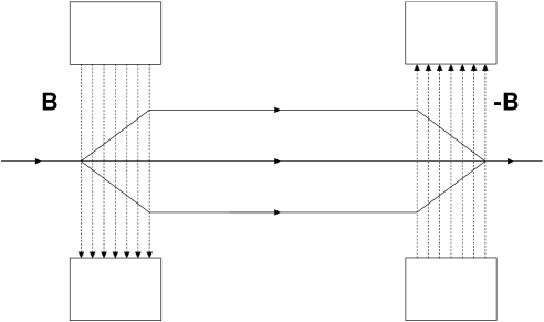
Figure 2: Stern-Gerlach Apparatus

The spin hilbert space $\cal{H}$ for a spin 1 particle is isomorphic to $\mathbb{C}^{3}$. Let $S_{x},~{}S_{y},~{}S{z}$ denote the observables corresponding to spin measurements in the x, y and z directions. Then we can choose a basis of $\cal{H}$, $\{|0,z\rangle,|+1,z\rangle,|-1,z\rangle\}$, in which $S_{z}$ is diagonal. $S_{x},~{}S_{y},~{}S_{z}$ are then represented by the standard $3\times 3$ spin matrices. A measurement of spin in the B direction corresponds to a basis in $\cal{H}$ consisting of the eigenvectors of ${\textbf{S.B}}=\text{B}_{x}S_{x}+\text{B}_{y}S_{y}+\text{B}_{z}S_{z}$. The eigenvectors of spin in the $x$ and $y$ directions are

$$|0,x\rangle= \frac{1}{\sqrt{2}}(|+1,z\rangle-|-1,z\rangle)\,,$$ (10)

$$|+1,x\rangle= \frac{1}{{2}}(|+1,z\rangle+\sqrt{2}|0,z\rangle+|-1,z\rangle)\,,$$ (11)

$$|-1,x\rangle= \frac{1}{{2}}(|+1,z\rangle-\sqrt{2}|0,z\rangle+|-1,z\rangle)\,,$$ (12)

$$|0,y\rangle= \frac{1}{\sqrt{2}}(|+1,z\rangle+|-1,z\rangle)\,,$$ (13)

$$|+1,y\rangle= \frac{1}{{2}}(|+1,z\rangle+i\sqrt{2}|0,z\rangle-|-1,z\rangle)\,,$$ (14)

$$|-1,y\rangle= \frac{1}{{2}}(|+1,z\rangle-i\sqrt{2}|0,z\rangle-|-1,z\rangle)\,.$$ (15)

5.2 Using Stern-Gerlach Apparatus to realise the Peres-Kochen-Specker setup

Instead of spin we will be interested in spin squared, i.e. $S_{i}^{2}$ in the $i$ direction (no sum on $i$). There are now two possible outcomes of a measurement, $S_{i}^{2}=0$ (corresponding to $S_{i}=0$) and $S_{i}^{2}=1$ (corresponding to $S_{i}=+1$ or $S_{i}=-1$). This can be mirrored within the Stern-Gerlach framework by lumping the two outer ($S_{i}=+1$ and $S_{i}=-1$) beams together and labelling them together as “the red beam” and labelling the middle beam as “the green beam”. This can be done “mentally” by simply ignoring the fine grained detail of which of the outer beams the particle is in, or “physically” by coherently recombining the two outer beams into a single beam using a reversed Stern-Gerlach apparatus (whilst keeping the middle beam separated by diverting it out of the way). Since in Anhomomorphic Logic we may not be able to reason (about fine and coarse graining for example) using classical rules, it will be clearer to assume that we have set up a physical recombiner so there really is a single “red beam” corresponding to $S_{i}^{2}=1$. Let us further imagine appending the exact reverse of this apparatus at the end which will coherently recombine the red and the green beams into a single beam again. We call this whole apparatus a “spin-squared beam splitter and recombiner (bsr) in the $i$ direction.”

For a spin-1 particle, $S_{i}^{2}$ and $S_{j}^{2}$ commute if the $i$ and $j$ directions are orthogonal, i.e. the squared $3\times 3$ spin representation matrices $\sigma_{x}^{2},~{}\sigma_{y}^{2},~{}\sigma_{z}^{2}$ commute. In the standard Copenhagen interpretation three (consecutive or simultaneous) spin-squared measurements in mutually orthogonal directions will necessarily result in one outcome of $0$ and two outcomes of $1$.

This can be seen directly in terms of projectors onto the relevant eigenspaces in the Hilbert space. Let $P_{i}^{0}=|0,i\rangle\langle 0,i|$ and $P_{i}^{1}={\bf 1}-P_{i}^{0}$, be projectors onto the spin-squared (in direction $i$) eigenspaces corresponding to eigenvalues 0 and 1 respectively. Then, looking at equations 10-15, we have $P_{i}^{0}P_{j}^{0}=0$ for any orthogonal pair of directions $i$ and $j$, and for a basis $u_{i},u_{j},u_{k}$ we have $P_{i}^{a}P_{j}^{b}P_{k}^{c}=0$ unless exactly one of $a$, $b$ or $c$ equals 0.

To translate this into spacetime paths, we imagine a spin-1 particle (in any spin state) passing through a sequence of three spin-squared bsr’s, one in each of the three orthogonal directions (no one of which coincides with the direction of motion of the particle). The classical realist picture is that the particle must pass through the green beam in exactly one bsr and through the red beam in the other two. We will see that the Peres-Kochen-Specker Theorem means that this is untenable.

We want to translate colourings of the entire Peres set $\{u_{i}\}$, not just one basis, into spacetime paths. We imagine a sequence of 33 spin-squared bsr’s in the directions $\{u_{i}\}$, so the first bsr will be in direction $u_{1}$, the second in $u_{2}$, etc. The particle trajectories form the space $\Omega$ in this setup and each one follows either the red or green beam through each bsr in turn and so every colouring can be realised by an element of $\Omega$. Strictly, there are many particle trajectories in each beam, with slight variations in positions, but we will ignore this finer grained detail and assume that $\Omega$ consists of the $2^{33}$ trajectories distinguished only by which beam is passed through in each bsr. This space is then in one-to-one correspondence with the space of colourings of the Peres Set and we identify the two in the obvious way, noting that the particle paths contain additional information, namely the choice of order of the Peres rays in the experimental set up, not present in the original space of colourings.

Let the initial spin state of the particle be $|\psi\rangle$. Then a decoherence functional, and hence a quantum measure, on $\Omega$ can be defined as follows. Let $\gamma$ be an element of $\Omega$, so $\gamma(u_{i})$ is a colour for each Peres direction $u_{i}$. As we saw above, colour “green” is identified with spin-squared value zero and colour “red” is identified with spin-squared value one. We can construct a “path state” $|\gamma\rangle$ via

$$|\gamma\rangle=P_{33}^{\gamma(u_{33})}\dots P_{2}^{\gamma(u_{2})}P_{1}^{\gamma(u_{1})}|\psi\rangle$$

where $P_{i}^{green}\equiv P_{i}^{0}$ and $P_{i}^{red}\equiv P_{i}^{1}$ are the projection operators defined previously. For each event $A\in{\hbox{\german A}}$ we can define an “event state”

$$|A\rangle=\sum_{\gamma\in A}|\gamma\rangle$$

and the decoherence functional is then defined by

$$D(A;B)=\langle A|B\rangle\,.$$

If the spin state of the particle is mixed the decoherence functional is a convex combination of such terms.

Claim 1.

The quantum measure on $\Omega$ defined as above values the PKS sets and their disjoint unions zero.

Proof.

Consider one of the PKS sets, $R_{\{u_{i},u_{j},u_{k}\}}$, say for a basis $\{u_{i},u_{j},u_{k}\}$. Then the “event state” $|R_{\{u_{i},u_{j},u_{k}\}}\rangle$ is given by a sum over “path states” $|\gamma\rangle$, one for each $\gamma$ in $R_{\{u_{i},u_{j},u_{k}\}}$. This sum involves a sum over the colouring of all the Peres rays which are not $u_{i}$, $u_{j}$ or $u_{k}$ and so the projection operators for all these rays sum to the identity and leave:

$$|R_{\{u_{i},u_{j},u_{k}\}}\rangle=P_{i}^{0}P_{j}^{0}P_{k}^{0}|\psi\rangle$$

which equals zero for any state $|\psi\rangle$ because the product of those projectors is zero. Similarly, the event state for each of the PKS sets is zero because it is a product of projectors acting on the initial state and that product of projectors is zero.

An event which is a disjoint union of PKS events has a corresponding event state which is a sum of terms, one for each PKS event in the union, each of which is zero.

Hence result. ∎

For a given initial state and a choice of ordering for the bsr’s we therefore have an explicit realisation of a quantum measure in which the PKS sets have measure zero. The statement of the Peres-Kochen-Specker theorem in the context of this gedankenexperiment is that every trajectory that a spin 1 particle can take through the apparatus is in one of the PKS precluded sets.

5.3 Physical Reality

Now consider the results of the previous section and their application to a quantum measure of the form constructed here (for some choice of linear ordering of the rays and a choice of initial state). The preclusion rule that we wish to impose requires that $|A|=0$ implies $\phi(A)=0$. The co-event $\phi_{M}$ and its rotations constructed in the previous section are preclusive on the PKS sets but they are not necessarily preclusive on any other events of measure zero that might arise. And there necessarily will be more sets of measure zero.

For example, if the choice of ordering of the Peres rays is such that two orthogonal rays are consecutive, then any element of $\Omega$ in which those two rays are coloured green will be a (singleton) measure zero set because the relevant projectors will be adjacent to each other and they are orthogonal. Similar “accidental” measure zero sets will arise whenever products of projectors that are zero are either there from the beginning in the choice of ordering or result from summing out intermediate projectors during coarse graining. There may be more measure zero sets, depending on $|\psi\rangle$, amongst the “inhomogeneous” sets i.e. those that are not constructed by summing over the sets of projectors for certain Peres rays.

We would like to use the co-event $\phi_{M}$ of the previous section and analyse the consequences of considering it as a potential reality. In order to make this analysis fully meaningful, therefore, we need to find a measure (an ordering of the rays and an initial state) such that $\phi_{M}$ is preclusive. This would be accomplished if the support of $\phi_{M}$, the set containing the two trajectories $\gamma_{P}$ and $\gamma_{P}^{\prime}$, was not contained in any set of measure zero. We believe that such a measure exists but we are not able to give a proof, the difficulty lying in the size of $\Omega$: $2^{33}$ colourings means that the number of possible measure zero sets is very large indeed.

We will, for the time being, assume that such a measure exists and analyse $\phi_{M}$ accordingly. In other words we assume that co-event $\phi_{M}$ is preclusive and so can describe “what actually happens” at the microscopic level in one run of the gedankenexperiment on a single particle. In that case, what of the question posed at the end of section 4?

Recall that in $\phi_{M}$ both the event “ray 021 is green” and the event “ray 021 is red” are false. Translated into spacetime terms we say that the particle is neither in the red beam nor in the green beam of the 021 bsr. The reason for this breakdown in the classical rule of inference is that, of the two elements of the support of $\phi_{M}$, $\gamma_{P}(021)=red$ and $\gamma_{P}^{\prime}(021)=green$. So neither redness nor greenness of ray 021 are common properties of the support of $\phi_{M}$ and so neither is a real property of the world.

Understanding how this comes about at the abstract level doesn’t however remove the uneasy feeling that there is a violation of known experimental facts here. Surely, whenever we check to see whether the particle is in the red beam or the green beam for any ray, by putting detectors in both beams for example, we find it in one or the other, not in neither. This would only be a contradiction, however, if such a measurement simply reveals, without altering, the microscopic reality. But, as is well known, the presence of detectors alters the measure by destroying coherence between beams and so will change the possible co-events. The presence of detectors in the 021 bsr will alter the measure so that the $\phi_{M}$ co-event will no longer be preclusive and no longer a possible reality.

It is tempting to call this “contextuality”: the microscopic reality depends on the experimental setup. Contextuality always sets up a threat to (what in the literature is called) locality and it is easy to see how that can occur: the “context” on which real events over here depend could be the experimental setting of a distant apparatus over there. In order to study this, we can consider a system of two spin 1 particles in a spin zero state so that their spin squared values are perfectly correlated. These two particles are sent to distant laboratories where they each pass through an identical Peres-Kochen-Specker apparatus of 33 bsr’s as described above. This is under investigation.

Note that there is one case in which placing detectors in both beams of the 021 bsr would not alter the measure and so would reveal the underlying microscopic reality without changing it. That is if the 021 bsr is the last one in the sequence, if 021 were the 33rd ray, $u_{33}$. However, in this case, $\phi_{M}$ would not be preclusive for the following reason. $\gamma_{P}$ corresponds to a product of projectors (a “class operator”) and three of those projectors are onto $red$ for the three rays in the basis $B_{11}$, one of which is $021$ and at the very end of the product. $\gamma_{P}$ is therefore in a set of measure zero which corresponds to summing over the projectors (coarse graining over the colours) for all the rays in between the three $B_{11}$ rays. The class operator for $\gamma_{P}^{\prime}$, on the other hand, contains three projectors onto $red$ for the basis rays in $B_{7}$ and so $\gamma_{P}^{\prime}$ is contained in a set of measure zero that corresponds to summing over the projectors for all the rays in between the three $B_{7}$ rays. These two measure zero sets are disjoint, because $\gamma_{P}(u_{33})=red$ and $\gamma_{P}(u_{33})=green$ and the 33rd projector is not summed over because it is at the end and not between any of the relevant projectors. The disjoint union of these two measure zero sets is measure zero and it contains both $\gamma_{P}$ and $\gamma_{P}^{\prime}$, the support of $\phi_{M}$. $\phi_{M}$ is, therefore, not a possible reality for this experimental setup and there is no contradiction with experimental facts.

This result – that no violations of classical rules of inference can occur when restricting attention to events that occur at the final time – is a special case of a more general theorem of Sorkin which will appear in a separate work.

6 Discussion

We have reviewed Sorkin’s Multiplicative Schemes for anhomomorphic logic in quantum measure theory. We have shown how to cast the Peres version of the Kochen-Specker theorem into the framework of quantum measure theory and described a Peres-Kochen-Specker gedankenexperiment as a sequence of 33 beam-splitters and recombiners (bsl). Certain subsets of paths of a spin 1 particle through this apparatus have measure zero and are precluded and the Peres-Kochen-Specker theorem says that the union of these subsets is the whole space of paths, $\Omega$. Therefore no single path can be real.

We constructed explicit primitive co-events in the Multiplicative Scheme which respect the PKS preclusions however we do not know if there are quantum measures for real experimental setups for which these co-events respect all the preclusions. We nevertheless used one of these explicit co-events to begin an analysis of issues such as contextuality in the scheme.

We present these results as an indication of the sorts of questions that arise as we struggle towards an interpretation of Quantum Measure Theory. To investigate further, we need to study examples of experimental situations for much simpler “quantum antimonies” for which all the measure zero sets can be explicitly found and all the primitive co-events calculated. This is being done and an example due to Hardy [16, 17] has been analysed by Furey and Sorkin [18]. We also need to work towards a measurement theory: any realistic interpretation of quantum mechanics worth its salt must be able to reproduce the predictions of Copenhagen quantum mechanics in the laboratory.

One motivation for pursuing this line of research is the desire to restore objective reality to physics, so that microscopic events can be understood to be just as real as macroscopic ones. The present authors are further motivated by the expectation that the correct interpretation of quantum mechanics will lead to advances in new physics and specifically in quantum gravity. It may, in particular, hold the explanation of how – Bell’s inequalities notwithstanding – physics can be both quantal and relativistically causal. The reason that the framework of quantum measure theory and anhomomorphic logic holds out this possibility is that it incorporates real events that have no probability distribution on them. It is possible then that such quantal events could be the “common causes” of the Bell Inequality violating correlations. Such a development could then lead to a formulation of a causal quantum dynamics for spacetime itself, along the lines of the formulation of causal classical stochastic dynamics [19]. Turning this around, perhaps fruitfulness for quantum gravity is the criterion whereby the correct interpretation of quantum mechanics will eventually be recognised.

7 Acknowledgments

We thank Rafael Sorkin for help and discussions throughout the course of this work. YG is supported by a PPARC studentship. FD is supported in part by the EC Marie Curie Research and Training Network, Random Geometry and Random Matrices MRTN-CT-2004-005616 (ENRAGE) and by Royal Society International Joint Project 2006/R2. FD thanks the Perimeter Institute for Theoretical Physics for hospitality during the latter stages of this work.

References

- [1] J. B. Hartle, The space time approach to quantum mechanics, Vistas Astron. 37 (1993) 569, [gr-qc/9210004].
- [2] P. A. M. Dirac, The Lagrangian in quantum mechanics, Physikalische Zeitschrift der Sowjetunion 3 (1933) 64–72.
- [3] R. P. Feynman, Space-time approach to nonrelativistic quantum mechanics, Rev. Mod. Phys. 20 (1948) 367.
- [4] R. P. Feynman, The development of the space-time view of quantum electrodynamics, 1965. Nobel Lecture, 1965, http://nobelprize.org/nobel_prizes/physics/laureates/1965/feynman-lecture.html.
- [5] J. B. Hartle, The quantum mechanics of cosmology, in Quantum Cosmology and Baby Universes: Proceedings of the 1989 Jerusalem Winter School for Theoretical Physics (S. Coleman, J. B. Hartle, T. Piran, and S. Weinberg, eds.), World Scientific, Singapore, 1991.
- [6] J. B. Hartle, Space-time quantum mechanics and the quantum mechanics of space-time, in Proceedings of the Les Houches Summer School on Gravitation and Quantizations, Les Houches, France, 6 Jul - 1 Aug 1992 (J. Zinn-Justin and B. Julia, eds.), North-Holland, 1995. gr-qc/9304006.
- [7] R. D. Sorkin, Quantum dynamics without the wave function, J. Phys. A40 (2007) 3207–3222, [quant-ph/0610204].
- [8] R. D. Sorkin, An exercise in “anhomomorphic logic”, 2007. to appear in a special volume of Journal of Physics, edited by L. Diósi, H-T Elze, and G. Vitiello, [quant-ph/0703276].
- [9] S. Kochen and E. Specker, The problem of hidden variables in quantum mechanics, J. Math. Mech. 17 (1967) 59–83.
- [10] R. Geroch, The Everett interpretation, Nous 18 (1984) 617.
- [11] G. Shafer and V. Vovk, “The origins and legacy of Kolmogorov’s “Grundbegriffe”.” Working Paper # 4, The Game-Theoretic Probability and Finance Project; http://www.probabilityandfinance.com, 2005.
- [12] R. D. Sorkin, Quantum mechanics as quantum measure theory, Mod. Phys. Lett. A9 (1994) 3119–3128, [gr-qc/9401003].
- [13] J. B. Hartle, Generalizing quantum mechanics for quantum spacetime, gr-qc/0602013. Contribution to the 23rd Solvay Conference, The Quantum Structure of Space and Time.
- [14] A. Peres, Two simple proofs of the Kochen-Specker theorem, J. Phys. A: Math. Gen. 24 (1991) L175–L178.
- [15] J. Conway and S. Kochen, “The free will theorem.” [quant-ph/0604079], 2006.
- [16] L. Hardy, Quantum mechanics, local realistic theories and Lorentz-invariant realistic theories, Phys. Rev. Lett. 68 (1992) 2981–2984.
- [17] L. Hardy, Nonlocality for two particles without inequalities for almost all entangled states, Phys. Rev. Lett. 71 (1993) 1665–1668.
- [18] C. Furey and R. D. Sorkin, “Anhomomorphic Co-events and the Hardy Thought Experiment.” In preparation.
- [19] D. P. Rideout and R. D. Sorkin, A classical sequential growth dynamics for causal sets, Phys. Rev. D61 (2000) 024002, [gr-qc/9904062].