Routing in Outer Space:
Improved Security and Energy-Efficiency
in Multi-Hop Wireless Networks

Abstract

In this paper we consider security-related and energy-efficiency issues in multi-hop wireless networks. We start our work from the observation, known in the literature, that shortest path routing creates congested areas in multi-hop wireless networks. These areas are critical—they generate both security and energy efficiency issues. We attack these problems and set out routing in outer space, a new routing mechanism that transforms any shortest path routing protocol (or approximated versions of it) into a new protocol that, in case of uniform traffic, guarantees that every node of the network is responsible for relaying the same number of messages, on expectation. We can show that a network that uses routing in outer space does not have congested areas, does not have the associated security-related issues, does not encourage selfish positioning, and, in spite of using more energy globally, lives longer of the same network using the original routing protocol.

I Introduction

During the past years the interest in multi-hop wireless networks has been growing significantly. These types of networks have an important functionality that is the possibility to use other nodes as relays in order to deliver messages and data from sources to destinations. This functionality makes multi-hop wireless networks not only scalable but also usable in various areas and contexts. One of the most representative and important examples of multi-hop wireless networks are wireless sensor networks where small devices equipped with a radio transmitter and a battery are deployed in an geographic area for monitoring or measuring of some desired property like temperature, pressure etc. [1, 2].

The routing on a wireless sensor network is one of the most interesting and difficult issues to solve due to the limited resources and capacities of the nodes. Hence, protocols that use less information possible and need minimal energy consumption of nodes have become more than valuable in this context. Much research work has been devoted to finding energy-efficient routing protocols for this kind of networks. Often, these protocols tend to find an approximation of the shortest path between the source and the destination of the message. In [3], the authors analyze the impact of shortest path routing in a large multi-hop wireless network. They show that relay traffic induces congested areas in the network. If the traffic pattern is uniform, i. e. every message has a random source and a random destination uniformly and independently chosen, and the network area is a disk, then the center of the disk is a congested area, where the nodes has to relay much more messages that the other nodes of the network. We have the same problem if the network area is a square, or a rectangle, or any other two-dimensional convex surface. Our experiments show that, when using geographic routing [4] on a network deployed in a square, 25% of the messages are relayed by the nodes in a small central congested region whose area is $3\%$ of the total area of the square.

Congested areas are bad for a number of important reasons. They raise security-related issues: If a large number of messages are relayed by the nodes deployed in a relatively small congested region, then jamming can be a vicious attack. It is usually expensive to jam a large geographical area, it is much cheaper and effective to jam a small congested region. In the square, for example, it is enough to jam 3% of the network area to stop 25% of the messages. Moreover, if an attacker has the goal of getting control over as many communications as possible, then it is enough to control 3% of the network nodes to handle 25% of the messages.

There are also energy-efficiency issues: Aside from re-transmissions, that are costly and, in congested areas, often more frequent, the nodes have to relay a much larger number of messages. Therefore these nodes will die earlier than the other nodes in the network, exacerbating the problem for the nodes in the congested region that are still operational. In the long run, this results in holes in the network and in a faster, and less graceful, death of the system. Note that these problems are not solved by trying to balance the load just locally, as done by a few protocols in the literature (like GEAR [5], for example)—these protocols are useful, they can be used in any case (in our protocols as well), and are efficient in smoothing the energy requirements among neighbors, while they can’t do much against congested areas and they don’t help to alleviate the above discussed security-related issues.

Lastly, there are other concerns in the contexts where the nodes are carried by individual independent entities. In this paper we do not consider mobility. However, if the position of the node can be chosen by the node itself in such a way to maximize its own advantage, and if energy is an issue, then no node would stay in the center of the square, the highly congested region. If the nodes are selfish, an uneven distribution of load in the network area leads to an irregular distribution of the nodes—there is no point in positioning in the place where the battery is going to last the shortest. Selfish behavior is a recent concern in the network community and it is rapidly gaining importance [4, 6, 7]. Most of these contributions show how to devise mechanisms such that selfish nodes can’t help but truthfully execute the protocol. For the best of our knowledge, here we are raising a new concern, that can be important in mobile networks or whenever the position of the node can be an independent and selfish choice.

Solving these issues—security, energy-efficiency, and tolerance to (a particular case of) selfish behavior—is an important and non-trivial problem, and, at least partially, our goal. In this paper we attack this problem and set out routing in outer space, a new routing mechanism that transforms any shortest path routing protocol (or approximated versions of it) into a new protocol that, in case of uniform traffic, guarantees that every node of the network is responsible for relaying the same number of messages, on expectation. We can show that a network that uses routing in outer space does not have congested areas, does not have the associated security issues, and, in spite of using more energy globally, lives longer of the same network using the original routing protocol—that is, it is more energy-efficient. We support our claims by showing routing in outer space based on geographic routing, and performing a large set of experiments.

The rest of the paper is organized as follows: In Section II we report on the relevant literature in this area; in Section III we present the theoretical idea behind our work, we come up with routing in outer space and prove its mathematical properties; In Section IV, after describing our node and network assumptions and our simulation environment, we discuss on on the practical issues related in implementing routing in outer space starting from geographic routing; lastly, we present an extensive set of experiments, fully supporting our claims.

II Related Work

Routing in multi-hop wireless networks is one of most important, interesting, and challenging tasks due to network devices limitations and network dynamics. As a matter of fact this is one of the most studied topics in this area, and the literature on routing protocols for multi-hop wireless networks is vast. There have been proposed protocols that maintain routes continuously (based on distance vector) [8, 9, 10], that create routes on-demand [11, 12, 13] or a hybrid [14]. For a good survey and comparison see [15, 16]. Other examples of routing protocols for multi-hop wireless networks are those based on link-state like OLSR [17], etc.

Geographic routing or position-based routing, where nodes locally decide the next relay on the basis based on information obtained through some GPS (Global Positioning System) or other location determination techniques [18], seems to be one of the most feasible and studied approach. Examples of reasearch work on this approach are protocols like GEAR (Geographical Energy Aware Routing) [5], GAF (Geographical Adaptive Fidelity) [19]. For a good starting survey see [20].

All these protocols try to approximate shortest path between sources and destinations over the network. In [21], the authors analytically study the impact of shortest single path routing on a node by approximating single paths to line segments and characterizing the deviation of routes from line segments. However, one of the parameters in their model is not analytically quantified and would need to be estimated via simulations. In [22] the authors introduce an analytical model to evaluate the imposed load at a node by approximating a shortest path route to a narrow rectangle, where the load of a node is defined as the number of paths going through the node. The length of the rectangle is defined as the distance between source and destination and the width of the rectangle parameterizes the deviation of paths from the line segments between sources and destinations. However, since the number of nodes is not parameterized in the analytic model, the model does not provide an explicit relationship between the load and the number of nodes. In [3], the authors analyze the load for a homogeneous multi-hop wireless network for the case of straight line routing as in [23, 24, 21, 22, 25, 3] (where Shortest path routing is approximated to straight line routing in large multi-hop wireless networks). Assuming uniform traffic, in [3] the authors prove that relays induce so called hotspots or congested areas in the network. The creation of these types of congested areas not only affect the overall network throughput by generating energy-efficiency problems, but also create the serious security problems that we mentioned before. Of course, geographic routing (which, in dense networks, approximates the shortest path between source and destination) also suffers of the same problems. A lot of work has been done regarding to the energy-efficiency issues, and several approaches that try to solve the problem locally have been proposed like [5, 26, 27].

III Routing in Outer Space

We model the multi-hop wireless network as a undirected graph $G=(V,E)$, where $V$ is the set of nodes and $E$ is the set of edges. The nodes are ad-hoc deployed on the network area $S$. Formally, it is enough to assume that $S$ is a metric space with distance $d_{S}$ and that every node is a point on $S$. Given two nodes $u,v\in V$ deployed on $S$, we will denote the distance between their positions on the space with $d_{S}(u,v)$. The nodes have a transmission range $r$—two nodes $u,v\in V$ are connected by a wireless link $uv\in E$ if $d_{S}(u,v)\leq r$, that is, their distance is at most $r$. The common practice in the literature is to take a convex surface as $S$, usually a square, a rectangle, or a disk, with the usual Euclidean distance. In this paper we assume that the nodes know their position, either by being equipped with a GPS unit, or by using one of the many localization protocols [28, 29]. And that they know the boundaries of the network area $S$; this is possible either by pre-loading this information on the nodes before deployment, or by using one of the protocols in [30, 31, 32].

We started from the observation that shortest path routing on the square, or even an approximate version of it, generates congested areas on the center of the network. We have already discussed that this phenomenon is not desirable. The same problem is present on the rectangle, on the disk, and on any two dimensional convex deployment of the network, which is the common case in practice. Here, the idea is to relinquish shortest paths so as to get rid of congested areas, with the goal of improving security, energy efficiency, and tolerance to selfish behavior of the multi-hop wireless network. As the first step, we have to realize that there do exist metric spaces that do not present the problem. First, we need a formal definition of the key property of the metric space we are looking for.

Definition 1

Consider a multi-hop wireless network deployed on a space $S$. Fix a node $u$ and choose its position on $S$ arbitrarily. Then, deploy the other nodes of the network uniformly and independently at random. We will say that $S$ is symmetric if, chosen two nodes $v_{1}$ and $v_{2}$ uniformly at random in the network, the probability that $u$ is on the shortest path from $v_{1}$ to $v_{2}$ does not depend on its position.

Clearly, the disk is not a symmetric space as in the above definition. It has been clearly shown in [3]—if node $u$ is on the center of the circle or nearby, the probability that $u$ is traversed by a message routed along the shortest path from a random source node $v_{1}$ to a random destination $v_{2}$ is larger than that of a node away from the center of the network area. Clearly, the square has exactly the same problem. This claim is confirmed by our experiments: $25\%$ of the shortest paths traverse a relatively small central disk whose area is $3\%$ of the entire square.

To solve these problems, our idea is to map the network nodes onto a symmetric space (the outer space) through a mapping that preserves the initial network properties (such as distribution, number of nodes, and, with some limitations, distances between them). The second step is to route messages through the shortest paths as they are defined on the outer space. When the outer space and the corresponding mapping are clear from the context, we will call these paths the outer space shortest paths. Since the outer space is symmetric, we can actually prove that every node in the network has the same probability of being traversed by an outer space shortest path. In the following section we will see that, based on this idea, we can design practical routing protocols that do not have highly congested areas, weaker security, and all the problems we have been discussing here. Now, let’s make a step back and proceed formally.

Let $S$ be the original space where the network is deployed, and let $T$ be the outer space, an abstract space we use to describe routes, both metric spaces with respective distances $d_{S}$ and $d_{T}$. We are looking for a mapping function $\phi:S\mapsto T$ with the following properties:

1. $\phi$ is an injection;

2. if $x$ is a point taken uniformly at random on $S$, then $\phi(x)$ is also taken uniformly at random on $T$;

3. for every $r>0$, and every $u,v\in T$, $u\neq v$, if $d_{T}(\phi(u),\phi(v))\leq r$ then $d_{S}(u,v)\leq r$.

Property 1 guarantees that $\phi^{-1}$ is well-defined, Property 2 guarantees that a uniform traffic on $S$ is still a uniform traffic when mapped onto $T$ through $\phi$, and Property 3 says that paths on $T$ are paths on $S$, when mapped through $\phi^{-1}$. We’ll see later why these properties are important.

Definition 2

A mapping $\phi:S\longrightarrow T$ is fair if it enjoys Properties 1, 2, and 3.

Once such a fair mapping has been fixed, any message from node $u$ to node $v$ can be routed following the shortest path $\phi(u),\dotsc,\phi(v)$ between the images of $u$ and $v$ and through the images of the nodes of the network under $\phi$ on space $T$. Being $\phi$ a fair mapping, the path $\phi^{-1}(u),\dots,\phi^{-1}(v)$ is a well defined path on $S$. Indeed, $\phi^{-1}(u)$ is unique for all $u$, since $\phi$ is injective; and any two consecutive nodes in the shortest path on $T$ are neighbors in $S$ as well, thanks to Property 3. If $T$ is symmetric as in Definition 1, the routing through $\phi$ would be well distributed over $T$. Hence, this path can be used to route messages on $S$, giving as a result a homogeneous distribution of the message flow over all the original network area.

Theorem 1

Let $\phi:S\longrightarrow T$ be a mapping from source metric space $S$ to target metric space $T$. Assume that $\phi$ is fair and $T$ is symmetric. Fixed a node $u\in S$, deployed the other nodes of the network uniformly at random, and taken a source $v_{1}\in S$ and a destination $v_{2}\in S$ uniformly at random, the probability that the outer space shortest path $\phi^{-1}(v_{1}),\dots,\phi^{-1}(v_{2})$ traverses $u$ is independent of the position of $u$ on $S$.

The above theorem gives an important hint on how to build a routing protocol on a not symmetric network area, in such a way that the message flow is distributed homogeneously over all the network. What is needed is to determine a symmetric space (the outer space) and a fair mapping for it, and then to “transform” the shortest paths on the original network area into the corresponding outer space shortest paths.

We assume that the original network area is a square of side 1. An excellent candidate as a symmetric outer space is the torus. A torus is a 3-dimensional surface that we can model as $T=[0,t]\times[0,t]$. Let $u_{x}$ and $u_{y}$ be the coordinates of the position of node $u$ on the torus. We can endow $T$ with the following distance $d_{T}$:

$$d_{T}(u,v)=\sqrt{d_{x}^{2}+d_{y}^{2}},$$ (1)

where

$$d_{x} =\min\{\left|u_{x}-v_{x}\right|,t-\left|u_{x}-v_{x}\right|\},\;\textrm{and}$$ (2)

$$d_{y} =\min\{\left|u_{y},v_{y}\right|,t-\left|u_{y},v_{y}\right|\}.$$ (3)

The common way to visualize a torus is to consider a square, and then to fold it in such a way that the left side is glued together with the right side, and that the top side is glued together with the bottom side. In the following, we will picture the torus unfolded, just like a square, as it is commonly done to easily see this 3-dimensional surface as a 2-dimensional one.

Fact 1

A torus surface is symmetric as in Definition 1.

Clearly, virtually no wireless network in real life is deployed on a torus. Here, we are using the torus just as an abstract space. We are not making any unreasonable assumption on the nodes of the network being phisically placed on a torus like area with continuous boundaries, nor are we assuming that the network area becomes suddenly a torus. Indeed, we assume that the real network is deployed on the square, where the nodes close to one side cannot communicate with the nodes close to the opposite side. Crucially, the paths used to deliver the messages are computed as they are defined through a fair mapping onto the torus, the outer space. Coming back to our idea, now that the target symmetric outer space has been chosen, what is left to do is to find a fair mapping $\phi_{ST}$ from the square to the torus.

Let $S=[0,1]\times[0,1]$ be a square, and let $T=[0,2]\times[0,2]$ be a torus. As the mapping $\phi_{ST}$ from $S$ to $T$ we propose the following:

$\phi_{ST}((x,y))=(x^{\prime},y^{\prime})$ where:

$$x^{\prime}=\begin{cases}x&\textrm{with probability }1/2\\ 2-x&\textrm{with probability }1/2,\end{cases}$$

and

$$y^{\prime}=\begin{cases}y&\textrm{with probability }1/2\\ 2-y&\textrm{with probability }1/2.\end{cases}$$

An example of such a mapping can be seen in Figure 1, where a node on the square is mapped to one of the four equally probably images on the torus.

Figure 1: Example of transformation of a point from the square to the torus through the mapping $\phi_{ST}$. Point $(x,y)$ on the square $S=[0,1]\times[0,1]$ has four possible and equally probable images on the torus $T=[0,2]\times[0,2]$. According on $\phi_{ST}$, only one of the images will actually appear on $T$.

Theorem 2

$\phi_{ST}$ is a fair mapping with probability one.

Proof:

The proof of this claim follows directly from the definition of the mapping $\phi_{ST}$. The full proof is technical, without adding much to the understanding of this work. Therefore, for the sake of brevity, we omit the details. ∎

It is interesting to note that it is not true that two points that are neighbors on the square are also neighbors on the torus when mapped through $\phi_{ST}$. Generally speaking, it is impossible to build a mapping with both this property and Property 3, since the square and the torus are topologically different.

The outer space shortest path between two nodes may be different from the corresponding shortest path. Clearly, it can’t be shorter by definition of shortest path on $S$. A natural question to ask is whether we can bound the stretch, that is, how much longer may the outer space shortest path be compared with the corresponding shortest path? Unfortunately, the answer is that the stretch cannot be bounded by a constant. However, quite surprisingly, we can prove a very good constant bound in the case when many messages are sent through the network, that is the common case in practice. Indeed, while in the worst case the stretch can be high, it is not on average if we assume a uniform traffic. This claim is formalized in the following theorem, where we show that, on expectation, the distance of the images under $\phi_{ST}$ of two nodes taken uniformly and independently at random is at most the double of the original distance.

Theorem 3

If $u,v$ are taken uniformly at random on the square $S=[0,1]\times[0,1]$, and $\phi_{ST}(u),\phi_{ST}(v)$ are their respective images under $\phi_{ST}$ on the torus $T=[0,2]\times[0,2]$, then

$$E[d_{T}(\phi_{ST}(u),\phi_{ST}(v)]\leq 2E[d_{S}(u,v)].$$

Proof:

Let $u,v\in S$ be two nodes whose position is taken uniformly at random, and let $E[d_{S}(u,v)]=\mu$ be the expectation of their distance on $S$. Since $\phi_{ST}$ is fair, also $\phi_{ST}(u)$ and $\phi_{ST}(v)$ are taken uniformly at random in the torus. Clearly, the distance between $\phi_{ST}(u)$ and $\phi_{ST}(v)$ on the torus cannot be larger of the distance of $\phi_{ST}(u)$ and $\phi_{ST}(v)$ on a square $S^{\prime}=[0,2]\times[0,2]$. Indeed, every path on the torus is also a path on the square (the opposite is not true); and the average distance of two random points in a square of edge two is the double of the average distance of two random points in a square of edge one. Therefore,

$$E[d_{T}(\phi_{ST}(u),\phi_{ST}(v)] \leq E[d_{S^{\prime}}(\phi_{ST}(u),\phi_{ST}(v)]$$

$$=2E[d_{S}(u,v)]$$

$$=2\mu.$$

∎

In the following, we will see with experiments that the actual average stretch is even smaller.

Of course, it is always possible to use the outer space shortest path only when the stretch of that particular path is small, and to use the classical shortest path when the stretch is high and the outer space shortest path is going to cost a lot more. However, we do not perform these kind of optimizations—even though they may reduce the global energy required by the network to deliver the messages, they also unbalance the load among the nodes. In the following, we will implement our idea in a practical routing protocol derived from geographical routing, and show its performance by means of experiments.

IV Routing in Outer Space in Practice

(a) Geographic routing between node $u$ and $v$.

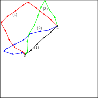
(b) Four equally probable outer space geographic routings between node $u$ and node $v$.

Figure 2: Transformation of a geographic route on the square into four possible outer space geographic routes between nodes $u$ and $v$. As can be seen, depending on which possible $\phi_{ST}(u)$ and $\phi_{ST}(v)$ images are chosen for $u$ and $v$ on the torus surface, there are four possible outer space geographic routes on the square between $u$ and $v$. The network is made of $6,441$ nodes.

In order to design a practical protocol that makes use of our ideas we start from geographic routing, a simple protocol that, when the network is dense enough, can be shown to approximate shortest path routing quite well [4]. Here, we define outer space geographic routing, its outer space counterpart.

In geographic routing, the destination of a message is a geographical position in the network area—in the square in our case. Every relay node performs a very simple protocol: send the message to the node that is closer to destination. If such a node does not exist, then the message is delivered. If the network is dense, every message is delivered to the node closest to destination. It is known that this simple version of geographic routing sometimes is not able to deliver the message to the node closest to destination, and there are plenty of ways to overcome this problem in the literature. However, we do not consider these extensions (outer space geographic routing could as well be based on these more complex and complete versions), since the increased complexity do not add much to this work.

Outer space geographic routing works quite as simply. Every relay node looks at the destination $x$ of the message, and forwards it to the node $u$ that minimizes $d_{T}(\phi_{ST}(x),\phi_{ST}(u))$. Just like geographic routing, implemented on the outer space.

Take, as an example, a message from node $u$ destined to a geographic position close to node $v$. According to the definition of $\phi_{ST}$, each node on the square $S$ has four possible and equally probable images on the torus $T$. This implies that for each pair $u$, $v$ of nodes on $S$ there are four possible and equally probable pairs of images $\phi_{ST}(u)$, $\phi_{ST}(v)$ on $T$. This yields four possible and different outer space geographic routes between the images $u$ and $v$ under $\phi_{ST}$. Hence, between any two nodes on the square there is one out of four different and equally probable outer space routes. To see an example of the four routes, see Figure 2.

To implement such a routing, it is enough that the nodes know their position in the square. Then, computing $\phi_{ST}$ for itself and the neighbors is trivial and fast. Note that it is not really important that the nodes agree on which of the four possible images is actually chosen for any particular node (except for the destination, but the problem can easily be fixed). However, to get this agreement it is enough that every node uses the same pseudo-random number generator, seeded with the id of the node being mapped.

IV-A Node and Network Properties, Assumptions, and Simulation Environment

We model our network node as a sensor. A typical example can be the Mica2DOT node (outdoor range $150\textrm{m}$, 3V coin cell battery). These nodes have been widely used in sensor network academic research and real testbeds. For our experiments, we have considered networks with up to 10,000 nodes, distributed on a square of side $1,500\textrm{m}$. In the following, we will assume for the sake of simplicity that the side of the square is 1, and that the node transmission range is 0.1. The nodes are placed according to a Poisson distribution with density $\rho$, chosen in such a way that every node has 30–40 neighbors on average. This is a reasonable and commonly used density for this kind of networks.

We inject a uniform traffic in the network—every message has a random source and a random destination uniformly and independently chosen. This type of traffic distribution is highly used in the simulations, for example when the goal is to study network capacity limits, optimal routing, and security properties [23, 33, 34]. We assume that the nodes know their position on the network area. Therefore, they need to know both their absolute position, and their position within the square. The nodes can get the absolute position either in hardware, by using a GPS (Global Positioning System), or in software. There exist several techniques for location sensing like those based on proximity or triangulation using different types of signals like radio, infrared acoustic, etc. Based on these techniques, several location systems have been proposed in the literature like infrastructure-based localization systems [35, 36] and ad-hoc localization systems [28, 29]. In [18] you can find a survey on these systems. Once the absolute position is known, we can get the nodes to know their relative position within the square by pre-loading the information on the deployment area, or by using one of the several techniques for boundary detection based on geometry methods, statistical methods, and topological methods (see [30, 31, 32]).

In the next two sections we present the results of the experiments we have performed, comparing our routing scheme with geographic routing over the same networks and with the same set of messages to route. For the experiments we have used our own event-based simulator. The assumptions and network properties listed above have been exactly reflected in the behavior of the simulator.

IV-B Security-Related Experiments

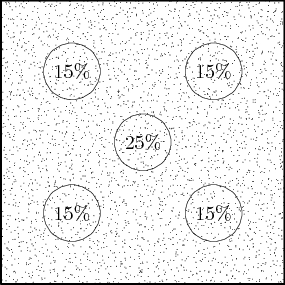
(a) Geographic routing.

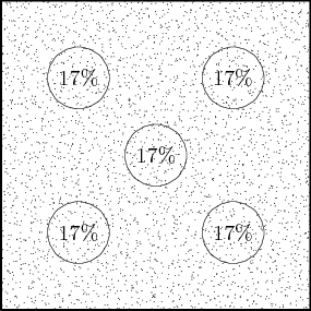
(b) Outer space geographic routing.

Figure 3: The average fraction of the messages whose routing path traverses the selected sub-areas of a network of $1,336$ nodes, in the case of geographic routing and in the case of outer space geographic routing.

In these experiments, we measure the number of messages whose routing path traverses five sub-areas of the same size in the network area. Every sub-area is a circle of radius $0.1$ (incidentally, the same of the transmission radius of a network node), that corresponds to an area of $3.14\%$ of the whole network surface. The sub-areas are centered in some “crucial” points of the network area: The center and the middle-half-diagonals points. The center of the network is known to be the most congested area. We want to test whether the middle-half-diagonal centered areas handle a significantly smaller number of messages. More specifically we consider the sub-areas centered in the points of coordinates $(0.5,0.5)$, $(0.25,0.25)$, $(0.25,0.75)$, $(0.75,0.25)$, $(0.75,0.75)$, assuming a square of side one. Our experiments are done on networks with different number of nodes (from 1,000 to 10,000). For each network we have launched both geographic routing and outer space geographic routing on message sets of different cardinality (from $50,000$ to $1,000,000$ of messages, generated as an instance of uniform traffic). In Figure 3 we present the average of the results obtained with a network of $1,336$ nodes generated by a Poisson process, but we stress out that exactly the same results are obtained for networks with up to $10,000$ nodes. As it can be seen, the experiments fully support the findings in [3]. Geographic routing (see Figure 3(a)) concentrates a relevant fraction of the messages on a small central area of the network, while the other sub-areas handle on average little more than the half. We have already discussed why this is dangerous, and important to avoid.

Figure 3(b) shows the result with the same set of messages and the same network deployment, this time using outer space geographic routing. The message load in the central sub-area is $30\%$ lower compared with the load of the same sub-area in the case of the geographic routing. Outer space geographic routing seems to transform the network area in a symmetric surface, making sure that the number of message handled by all the sub-areas remains reasonably low, $17\%$, and equally distributed. As a result, the load among network nodes is equally balanced and there are no “over-loaded” areas. This network is intuitively stronger than the same network using geographic routing, there are no areas that are clearly more rewarding as objective of a malicious attack, and no network areas have more “responsabilities” than others.

Furthermore, Figure 3(a) clearly shows that, with geographic routing, it is not a good strategy to stay in the center of the network if you want to save your battery. If the nodes are selfish, it is a much better strategy to position in one of the sub-central areas, for example, where the battery is going to last $66\%$ longer. Even better if you move towards the side of the square. Conversely, when using outer space geographic routing, there is no advantage in choosing one position or the other, which is exactly our goal to guarantee an even distribution of the nodes, although part of them are selfish.

IV-C How to Live Longer by Consuming More Energy

Our main motivation is related to security. However, it is always important to understand what is the energy overhead of getting rid of congested areas. Indeed, what Theorem 3 says in a word is that the paths using outer space geographic routing are on average (at most) twice as long as the paths using geographic routing. This should have an immediate consequence on energy consumption: Messages routed with outer space geographic routing should make network nodes consume more energy, up to twice as much. And it actually is so. What it turns out with our experiments is that the overall energy consumption is about $1.4$ times larger with outer space geographic routing, see Figure 4. Like before, the figure shows the result with a network of $1,625$ nodes, but we have done more experiments with different sizes, up to $10,000$ nodes, and the result does not change.

Usually, when a wireless network consumes more energy, its life is shorter. However, it is not always the case. Sometimes it is better to consume more energy, if this is done more equally in the network. This is exactly what happens with outer space geographic routing. We consider two measure of network longevity: time to first node death, time to loss of efficiency in delivery messages. These measures are well-known and used in the literature [37, 38, 39]. We have made two sets of experiments, each using one of the above way to measure the longevity of the network. In each of the experiments we count the number of messages that are successfully delivered before network “death”, where network death is defined according to the above two measures.

Figure 4: Global energy consumption of the network nodes after running geographic and outer space geographic routing, respectively, on sets of $50,000$ messages each.The network considered is made of $1,625$ nodes.

The first set of experiments is done according to the first measure. We have generated the network, the uniform traffic, and injected the traffic into two copies of the same network, one using geographic routing and one using outer space geographic routing. This have been iterated several times with networks of different sizes. The result is shown in Figure 5, where we show the number of messages delivered on average by a network of $1,625$ nodes (the result does not change by considering network of different size), using the two routing protocols under evaluation.

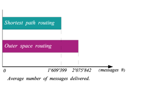
Figure 5: Time to first node death. The time is measured as the number of messages delivered to destination before the death of the first node. The network consists of $1,625$ nodes.

As you can see, the network lifetime of outer space geographic routing is $22.57\%$ longer, on average, than simple geographic routing. As a matter of fact, the number of messages successfully delivered by the network until the very first node death is much greater with outer space routing.

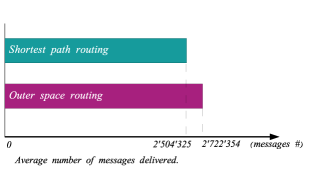
Figure 6: Time to delivered percentage. The time is measured as the number of messages delivered to destination before the delivery success ratio falls under $95\%$. The network considered is made of $1,625$ nodes.

Since security usually comes at a price, this is somewhat surprising. Routing in outer space seems to deliver a more secure routing and a more energy-efficient network, simultaneously.

Figure 6 shows the result we get when considering the second definition of network lifetime. In this case, we consider the network dead when it is not efficient any more in delivering messages. Note that geographic routing (and similarly its outer space version) has the problem of “dead ends”, places where the message cannot proceed because there is no node closer to destination, while the destination is still far. There are a number of solutions to this problem, and there do exists more sophisticated versions of geographic routing that know how to detect this situation and deliver the message whenever there is a path between source and destination. However, this mechanisms are usually costly. When the network is not able any longer to deliver messages with simple geographic routing, that means that there has been enough deterioration to create many dead ends in the network itself. We use this as a measure of the quality of its structure. In this set of experiments we count the number of messages that reach destination until the percentage of delivery falls under some threshold (in our case $95\%$). As can be seen in the figure, even in this case outer space geographic routing prolongs the life of the network to a value that is on average $11.14\%$ larger than the one achieved with geographic routing.

V Conclusions

Uniform traffic injected into multi-hop wireless networks generates congested areas. These areas carry a number of non-trivial issues about security, energy-efficiency, and tolerance to (a particular case of) selfish behavior. In this paper we describe routing in outer space, a mechanism to transform shortest path routing protocols into new protocols that do not have the above mentioned problems.

Routing in outer space guarantees that every node of the network is responsible for relaying the same number of messages, on expectation. We can show that a network that uses routing in outer space does not have congested areas, does not have the associated security-related issues, does not encourage selfish positioning, and, in spite of using more energy globally, lives longer of the same network using the original routing protocol.

References

- [1] I. Akyildiz, W. Su, Y. Sankarasubramaniam, and E. Cayirci, “A survey on sensor networks,” IEEE Communcations Magazine, vol. 40, pp. 102–114, August 2002.
- [2] A. Mainwaring, D. Culler, J. Polastre, R. Szewczyk, and J. Anderson, “Wireless sensor networks for habitat monitoring,” in WSNA ’02: Proceedings of the 1st ACM international workshop on Wireless sensor networks and applications, (New York, NY, USA), pp. 88–97, ACM Press, 2002.
- [3] S. Kwon and N. B. Shroff, “Paradox of shortest path routing for large multi-hop wireless networks,” in IEEE INFOCOM’07 Anchorage, May 2007.
- [4] B. Karp and H. T. Kung, “Gpsr: Greedy perimeter stateless routing for wireless networks,” in Proceedings of the 6th Annual ACM/IEEE International Conference on Mobile Computing and Networking (MobiCom ’00), (Boston, MA, USA), August 2000.
- [5] Y. Yu, R. Govindan, and D. Estrin, “Geographical and energy aware routing: A recursive data dissemination protocol for wireless sensor networks,” Tech. Rep. UCLA/CSD-TR-01-0023, UCLA Computer Science Department, May 2001.
- [6] V. Srinivasan, P. Neggehalli, C. F. Chiasserini, and R. R. Rao, “Cooperation in wireless ad hoc wireless networks,” in Proceedings of the Twenty-Second Annual Joint Conference of the IEEE Computer and Communications Societies (INFOCOM 2003), 2003.
- [7] W. Wang, X. Li, and Y. Wang, “Truthful multicast routing in selfish wireless networks,” in Proceedings of the 10th Annual ACM/IEEE International Conference on Mobile Computing and Networking (MobiCom ’04), (Philadelphia, PA, USA), September 2004.
- [8] C. E. Perkins and P. Bhagwat, “Highly dynamic destination-sequenced distance-vector routing (dsdv) for mobile computers,” in SIGCOMM ’94: Proceedings of the conference on Communications architectures, protocols and applications, (New York, NY, USA), pp. 234–244, ACM Press, 1994.
- [9] M. G. Zapata and N. Asokan, “Securing ad hoc routing protocols,” in Proceedings of the ACM Workshop on Wireles Security (WiSe), 2002.
- [10] K. Sanzgiri, B. Dahill, B. Levine, C. Shields, and E. Belding-Royer, “A secure routing protocol for ad hoc networks,” in Proceedings of the International Conference on Network Protocols (ICNP), 2002.
- [11] D. B. Johnson and D. A. Maltz, “Dynamic source routing in ad hoc wireless networks,” in Mobile Computing (Imielinski and Korth, eds.), vol. 353, Kluwer Academic Publishers, 1996.
- [12] V. D. Park and M. S. Corson, “A highly adaptive distributed routing algorithm for mobile wireless networks,” in INFOCOM ’97: Proceedings of the INFOCOM ’97. Sixteenth Annual Joint Conference of the IEEE Computer and Communications Societies. Driving the Information Revolution, (Washington, DC, USA), p. 1405, IEEE Computer Society, 1997.
- [13] C. Perkins and E. Royer, “Ad hoc on-demand distance vector routing,” in Proceedings of the IEEE Workshop on Mobile Computing Systems and Applications, pp. 90–100, February 1999.
- [14] Z. Haas, “A new routing protocol for the reconfigurable wireless networks,” in Proc. of the IEEE Int. Conf. on Universal Personal Communications, October 1997.
- [15] J. Broch, D. A. Maltz, D. B. Johnson, Y.-C. Hu, and J. Jetcheva, “A performance comparison of multi-hop wireless ad hoc network routing protocols,” in MobiCom ’98: Proceedings of the 4th annual ACM/IEEE international conference on Mobile computing and networking, (New York, NY, USA), pp. 85–97, ACM Press, 1998.
- [16] E. Royer and C. Toh, “A review of current routing protocols for ad-hoc mobile wireless networks,” April 1999.
- [17] P. Jacquet, P. Mühlethaler, T. Clausen, A. Laouiti, A. Qayyum, and L. Viennot, “Optimized link state routing protocol for ad hoc networks,” in Proceedings of the 5th IEEE Multi Topic Conference (INMIC 2001), 2001.
- [18] J. Hightower and G. Borriello, “Location systems for ubiquitous computing,” IEEE Computer, vol. 34, pp. 57–66, August 2001.
- [19] Y. Xu, J. Heidemann, and D. Estrin, “Geography-informed energy conservation for ad hoc routing,” in Proceedings of the 7th Annual ACM/IEEE International Conference on Mobile Computing and Networking (MobiCom ’01), (Rome, Italy), July 2001.
- [20] K. Seada and A. Helmy, “Geographic protocols in sensor networks,” tech. rep., USC, July 2004.
- [21] P. P. Pham and S. Perreau, “Increasing the network performance using multi-path routing mechanism with load balance,” Ad Hoc Networks, vol. 2, pp. 433–459, October 2004.
- [22] Y. Ganjali and A. Keshavarzian, “Load balancing in ad hoc networks: single-path routing vs. multi-path routing,” in Proceedings of the Twenty-third Annual Joint Conference of the IEEE Computer and Communications Societies (INFOCOM 2004), vol. 2, pp. 1120–1125 vol.2, 2004.
- [23] P. Gupta and P. R. Kumar, “The capacity of wireless networks,” IEEE Transactions On Information Theory, vol. 46, March 2000.
- [24] A. Rajeswaran and R. Negi, “Capacity of power constrained ad-hoc networks,” in Proceedings INFOCOM, 2004., vol. 1, pp. 7–11, March 2004.
- [25] M. Franceschetti, O. Dousse, D. Tse, and P. Thiran, “On the throughput capacity of random wireless networks,” IEEE Transactions on Information Theory, vol. 52, june 2006.
- [26] M. Zorzi and R. R. Rao, “Geographic random forwarding (geraf) for ad hoc and sensor networks: Energy and latency performance,” IEEE Transactions on Mobile Computing, vol. 2, no. 4, pp. 349–365, 2003.
- [27] P. Casari, A. Marcucci, M. Nati, C. Petrioli, and M. Zorzi, “A detailed simulation study of geographic random forwarding (geraf) in wireless sensor networks,” in Military Communications Conference, 2005. MILCOM 2005.IEEE, vol. 1, pp. 59–68, October 2005.
- [28] N. Bulusu, J. Heidemann, D. Estrin, and T. Tran, “Self–configuring localization systems: Design and experimental evaluation,” Trans. on Embedded Computing Sys., vol. 3, no. 1, pp. 24–60, 2004.
- [29] A. Savvides, C.-C. Han, and M. B. Srivastava, “Dynamic fine-grain localization in ad-hoc networks of sensors,” in Proceedings of the Seventh Annual ACM/IEEE International Conference on Mobile Computing and Networking (Mobicom), 2001.
- [30] Q. Fang, J. Gao, and L. J. Guibas, “Locating and bypassing holes in sensor networks,” Mob. Netw. Appl., vol. 11, no. 2, pp. 187–200, 2006.
- [31] A. Kröller, S. P. Fekete, D. Pfisterer, and S. Fischer, “Deterministic boundary recognition and topology extraction for large sensor networks,” in SODA ’06: Proceedings of the seventeenth annual ACM-SIAM symposium on Discrete algorithm, (New York, NY, USA), pp. 1000–1009, ACM Press, 2006.
- [32] Y. Wang, J. Gao, and J. S. Mitchell, “Boundary recognition in sensor networks by topological methods,” in MobiCom ’06: Proceedings of the 12th annual international conference on Mobile computing and networking, (New York, NY, USA), pp. 122–133, ACM Press, 2006.
- [33] A. Zemlianov and G. de Veciana, “Capacity of ad hoc wireless networks with infrastructure support,” IEEE Journal on selected areas in Communications, vol. 23, March 2005.
- [34] X. Hong, P. Wang, J. Kong, Q. Zheng, and J. Liu, “Effective probabilistic approach protecting sensor traffic,” Military Communications Conference, 2005. MILCOM 2005. IEEE, vol. 1, pp. 169–175, October 2005.
- [35] A. Ward, A. Jones, and A. Hopper, “A new location technique for the active office,” 1997.
- [36] N. Priyantha, A. Chakraborty, and H. Balakrishnan, “The cricket location-support system,” in Proceedings of the 6th Annual ACM International Conference on Mobile Computing and Networking (MobiCom ’00), August 2000.
- [37] M. Bhardwaj and A. Chandrakasan, “Bounding the lifetime of sensor networks via optimal role assignments,” in Proceedings of the Twenty-First Annual Joint Conference of the IEEE Computer and Communications Societies (INFOCOM 2002), vol. 3, pp. 1587–1596, 2002.
- [38] D. Blough and P. Santi, “Investigating upper bounds on network lifetime extension for cell-based energy conservation techniques in adhoc networks,” in Proceedings of the Eighth Annual International Conference on Mobile Computing and Networking (ACM MobiCom 2002), 2002.
- [39] H. Zhang and J. Hou, “On deriving the upper bound of —lifetime for large sensor networks,” in MobiHoc ’04: Proceedings of the 5th ACM international symposium on Mobile ad hoc networking and computing, (New York, NY, USA), pp. 121–132, ACM Press, 2004.