Dynamical feedback of the curvature drift instability on its saturation process

Abstract

Aims. We investigate the reconstruction of pulsar magnetospheres close to the light cylinder surface to study the curvature drift instability (CDI) responsible for the twisting of magnetic field lines in the mentioned zone. The influence of plasma dynamics on the saturation process of the CDI is studied.

Methods. On the basis of the Euler, continuity, and induction equations, we derive the increment of the CDI and analyze parametrically excited drift modes. The dynamics of the reconstruction of the pulsar magnetosphere is studied analytically.

Results. We show that there is a possibility of a parametrically excited rotational-energy pumping-process in the drift modes. It is indicated by the generation of a toroidal component of the magnetic field that transforms the field lines into such a configuration, in which plasma particles do not experience any forces. At this stage, the instability process saturates and the further amplification of the toroidal component to the magnetic field lines is suspended.

1 Introduction

Exploring the magnetic field of the Crab nebula, Piddington (1957) was the first to discover the presence of a central object in the nebula, with frozen magnetic field inside. It was assumed that the rotation of a central object provokes the generation of the toroidal component of magnetic field. Investigations have also shown that this kind of magnetic field characterizes magnetized star outflows (Weber & Davis (1967)). Pulsars are one of the most distinctive examples of rotationally powered magnetized stars producing the relativistic outflows commonly known as pulsar winds.

One of the major problems for pulsar winds concerns the transition of the magnetized plasma flows by means of the so-called ”light cylinder” surface, a hypothetical zone, where the linear velocity of rotation equals the speed of light. According to the model of pulsar magnetosphere (Goldreich & Julian (1969)), the relativistic plasma flow, emanating from the pulsar surface streams along very strong magnetic field lines. The typical values of the magnetic field are of the order of $10^{12}$ G (Manchester & Taylor (1977)). Such a strong magnetic field forces the particles, streaming toward the light cylinder zone, to co-rotate with a pulsar. On the other hand, once the relativistic effect of the mass increment is taken into account, the radial acceleration of the particles appears to be limited. This means that the particles will never cross the light cylinder surface if the rigid rotation is preserved (Machabeli & Rogava (1994)). Therefore, the co-rotation of the magnetized plasma cannot be maintained close to the mentioned zone and a further exploration of this phenomenon is needed.

The simplest means of explaining the transition in the plasma outflow at the light cylinder surface is to constrain the motion of the flow to become asymptotically close to a regime, in which particles do not experience any forces (see e.g., Machabeli et al. (2000); Rogava et al. (2003)). For this purpose, if the magnetic field is still strong, one needs to twist the field lines in an appropriate way. In other words, it is necessary to generate the toroidal component of the magnetic field. The pulsars maintain the dipolar magnetic field with a certain curvature of the field lines. The particles moving along the curved field lines drift perpendicularly to the curvature plane. The existence of the drift motion creates the necessary conditions for developing a CDI (see e.g., Kazbegi et al. (1989); Kazbegi et al. 1991a ; Kazbegi et al. 1991b ; Shapakidze et. al (2003)). The mechanism excites transverse drift modes providing the magnetic field with the toroidal component. The CDI becomes effective in the vicinity of the light cylinder surface, where the pulsar’s dipolar field is comparable to the toroidal component of the excited mode. The kinetic energy of the primary beam particles, of Goldreich-Julian (GJ) density, can indeed supply the generation of the drift waves. Mostly, it is assumed that the toroidal component of the magnetic field is created by the GJ current. However, the kinetic energy density, ${W}_{b}$, of the primary beam is insufficient to change the configuration of the dipolar magnetic field, $B_{0}$, significantly, since ${W}_{b}<<B_{0}^{2}/(4\pi)$. Therefore, the process of generating the toroidal component, $B_{r}$ (of the order of $B_{0}$), requires an additional energy supply, which can be extracted from the pulsar rotational energy. We have already shown that the rotational energy pumping into the drift modes can be implemented by the ”parametric” instability (Osmanov et al. (2008)). This mechanism is called parametric, because the effect is caused by the relativistic centrifugal force, which, as a parameter, changes in time and induces the instability. The aim of the present paper is to study the saturation process of this instability close to the light cylinder zone.

The problem analysis is completed well if one considers the mechanical analog of the motion of plasma flow along the pulsar magnetic field lines and studies the dynamics of a single particle moving inside the rotating channels. In the present paper, we apply the method developed in (Rogava et al. (2003)) and study the plasma process that converts the configuration of the magnetic field lines to the Archimedes’ spiral: it appears that in order to suppress the reaction force, the field lines, rather being straight, should deviate back and lag behind the rotation; consequently, the curvature will eventually increase, inevitably leading to the decrement of the reaction force; this process will last until the magnetic field lines form the shape of the Archimedes’ spiral, which removes the reaction force and saturates the instability.

The paper is arranged as follows. In section 2, we examine the parametric curvature drift instability and derive an expression for its corresponding growth rate. In section 3, we consider the kinematics of a particle moving along the rotating magnetic field line. In section 4, we apply the method for 1-second pulsars and the Crab pulsar, and in section 5 we summarize our results.

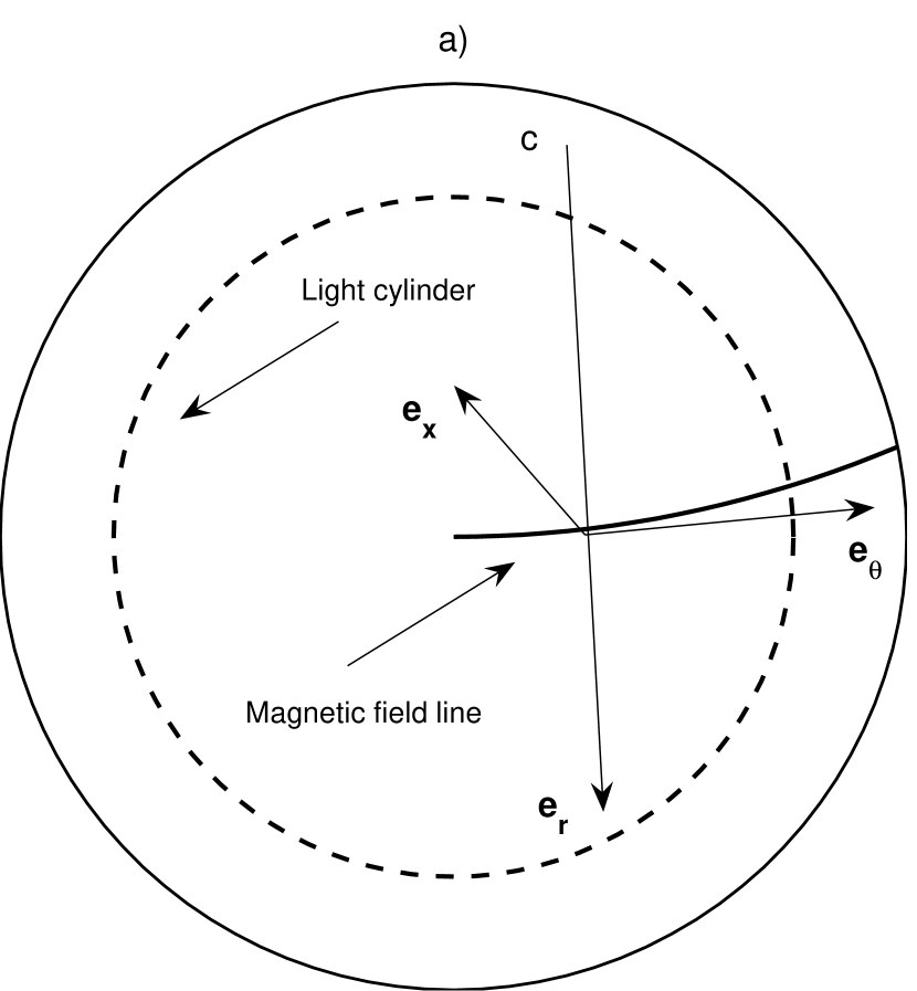
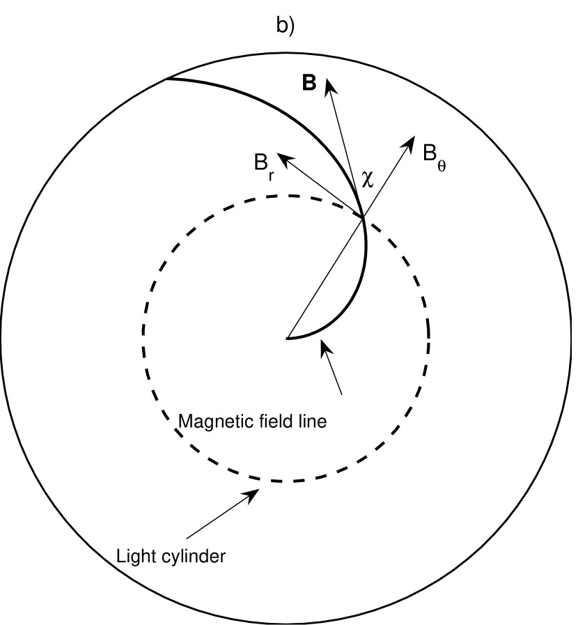
Figure 1: $a$) The geometry in which the set of main Eqs. (1-3) is considered; (${\bf e}_{\theta},{\bf e}_{r},{\bf e}_{x}$) denotes orthonormal basis of unit vectors; ${\bf e}_{x}$ is directed perpendicularly to the plane of the figure; $C$ is the center of the curvature; and ${\bf e}_{\theta}$ and ${\bf e}_{r}$ are the tangential and perpendicular (with respect to the field line) unit vectors respectively. $b$) The geometry for deriving Eq. (23): the curved line denotes the twisted magnetic field, ${\bf B}$, generated due to the raising of magnetic perturbation, ${\bf B}_{r}$. Note, that ${\bf B}_{r}$ and ${\bf B}_{\theta}$ are oriented with respect to the initial ‘quasi straight’ magnetic field line.

2 Parametric curvature drift instability

It is well known that the presence of an external varying parameter usually generates the plasma instability. For example, the mechanism of energy pumping process from the external alternating electric field into the electron-ion plasma is quite well investigated (see e.g., Silin (1973); Galeev & Sagdeev (1973); Max (1973)). Although the physics of the parametric instability in the electron-ion plasma differs from that of the electron-positron ($e^{-}e^{+}$) plasma, the techniques of calculation can be the same. The case of a $e^{-}e^{+}$ plasma, where the external varying parameter is the altering centrifugal acceleration, was considered by Machabeli et al. (2005).

We start our consideration by initially assuming that the magnetic field lines are almost straight with very small non zero curvature (see Fig. 1a). The plasma stream is supposed to move along the co-rotating field lines of a very strong magnetic field ($\sim 10^{12}$ G for typical pulsars). We assume that the plasma flow consists of two components: the plasma component composed of electrons and positrons ($e^{\pm}$); and, the so-called, beam component ($b$) composed of ultra relativistic electrons. The dynamics of plasma particles moving along the straight rotating magnetic field lines is described by the Euler equation (Machabeli et al. (2005))

$$\frac{\partial{\bf p_{\alpha}}}{\partial t}+({\bf v_{\alpha}\nabla)p_{\alpha}}=-c^{2}\gamma_{\alpha}\xi{\bf\nabla}\xi+\frac{e_{\alpha}}{m}\left({\bf E}+\frac{1}{c}\bf v_{\alpha}\times\bf B\right),$$ (1)

where

$$\xi\equiv\sqrt{1-\Omega^{2}R^{2}/c^{2}}\,,$$

$R$ is the coordinate along the straight field lines, $\alpha=\{e^{\pm},b\}$ denotes the sort of particles, ${\bf p_{\alpha}}$, ${\bf v_{\alpha}}$, and $e_{\alpha}$ are the momentum (normalized to the particle’s mass), the velocity, and the charge of electrons/positrons, respectively; ${\bf E}$ is the electric field and ${\bf B}$ is the magnetic field. On the right-hand side of Eq. (1), there are two major terms, the first of which represents the centrifugal force and the second, the Lorentz force. The full set of equations for $n,{\bf v},{\bf E}$, and ${\bf B}$ should be completed by the continuity equation

$$\frac{\partial n_{\alpha}}{\partial t}+{\bf\nabla}(n_{\alpha}{\bf v_{\alpha}})=0,$$ (2)

and the induction equation

$${\bf\nabla\times B}=\frac{1}{c}\frac{\partial{\bf E}}{\partial t}+\frac{4\pi}{c}\sum_{\alpha=e^{\pm},b}{\bf J_{\alpha}},$$ (3)

where $n_{\alpha}$ and ${\bf J_{\alpha}}$ are the density and the current, respectively.

Rewriting the Euler equation in Eq. (1) for the leading state and taking into account the frozen-in condition ${\bf E}_{0}+\frac{1}{c}{\bf v}_{0\alpha}\times{\bf B}_{0}=0$, the solution for ultra relativistic particle velocities writes as follows (Machabeli & Rogava (1994))

$$v^{0}_{\theta}\equiv v_{{}_{\parallel}}=c\,\cos(\Omega t+\varphi),$$ (4)

where $v_{{}_{\parallel}}$ denotes the velocity component along the magnetic field lines and $\varphi$, the initial phase of each particle.

The centrifugal force eventually causes the separation of charges in plasma consisting of several species. This process becomes so important that the corresponding electromagnetic field affects the dynamics of the charged particles. Therefore, the produced electric field should also be considered in Eq. (1) as the next term to be approximated (Osmanov et al. (2008)).

To clarify the mathematical treatment, we linearize the set of Eqs. (1-3), assuming that, to the zeroth approximation, the flow has a longitudinal velocity satisfying Eq. (4) and also drifts along the $x$-axis because of the curvature of magnetic field lines (see Fig. 1):

$$u_{\alpha}=\frac{\gamma_{\alpha_{0}}v_{{}_{\parallel}}^{2}}{\omega_{B_{\alpha}}R_{B}},$$ (5)

where $u_{\alpha}$ is the drift velocity; $\omega_{B_{\alpha}}=e_{\alpha}B_{0}/mc$, $R_{B}$ is the curvature radius of magnetic field lines, and $B_{0}$ is the magnetic induction in the leading state. In our case, the curvature drift contributes to ${\bf J}$ [see Eq. (3)] as a source of additional current.

We represent all physical quantities as the sum of the zeroth and the first order terms

$$\Psi\approx\Psi^{0}+\Psi^{1},$$ (6)

where

$$\Psi\equiv\{n,{\bf v},{\bf p},{\bf E},{\bf B}\}.$$

We then express the perturbed quantities as

$$\Psi^{1}(t,{\bf r})\propto\Psi^{1}(t)\exp\left[i\left({\bf kr}\right)\right]\,,$$ (7)

examining only the $x$ components of Eqs. (1,3), considering the perturbations with $k_{\theta}\ll k_{x}$ and $k_{r}=0$, and bearing in mind that $v^{1}_{r}\approx cE^{1}_{x}/B_{0}$, one can easily reduce the set of Eqs. (1-3) to the form

$$\frac{\partial p^{1}_{{\alpha}_{x}}}{\partial t}-i(k_{x}u_{\alpha}+k_{\theta}v_{{}_{\parallel}})p^{1}_{{\alpha}_{x}}=\frac{e_{\alpha}}{mc}v_{{}_{\parallel}}B^{1}_{r},$$ (8)

$$\frac{\partial n^{1}_{\alpha}}{\partial t}-i(k_{x}u_{\alpha}+k_{\theta}v_{{}_{\parallel}})n^{1}_{\alpha}=ik_{x}n_{\alpha}^{0}v^{1}_{\alpha_{x}},$$ (9)

$$-ik_{\theta}cB^{1}_{r}=4\pi\sum_{\alpha=e^{\pm},b}e_{\alpha}(n_{\alpha}^{0}v^{1}_{\alpha_{x}}+n_{\alpha}^{1}u_{\alpha}).$$ (10)

Introducing a special ansatz for $v^{1}_{\alpha_{x}}$ and $n^{1}_{\alpha}$

$$v^{1}_{\alpha_{x}}\equiv V_{\alpha_{x}}e^{i{\bf kA_{\alpha}(t)}},$$ (11)

$$n^{1}_{\alpha}\equiv N_{\alpha}e^{i{\bf kA_{\alpha}}(t)},$$ (12)

where

$$A_{\alpha_{x}}(t)=\frac{u_{\alpha}}{2\Omega}\left(\Omega t+\varphi\right)+\frac{u_{\alpha}}{4\Omega}\sin[2\left(\Omega t+\varphi\right)],$$ (13)

$$A_{\alpha_{\theta}}(t)=\frac{c}{\Omega}\sin(\Omega t+\varphi),$$ (14)

and substituting Eqs. (11,12) into Eqs. (8,9), one derives the expressions

$$v^{1}_{{\alpha}_{x}}=\frac{e_{\alpha}}{mc\gamma_{\alpha_{0}}}{\rm e}^{i{\bf kA_{\alpha}}(t)}\int^{t}{\rm e}^{-i{\bf kA_{\alpha}}(t^{\prime})}v_{{}_{\parallel}}(t^{\prime})B_{r}(t^{\prime})dt^{\prime},$$ (15)

$$n^{1}_{\alpha}=\frac{ie_{\alpha}n_{{\alpha}}^{0}k_{x}}{mc\gamma_{\alpha_{0}}}{\rm e}^{i{\bf kA_{\alpha}}(t)}\int^{t}dt^{\prime}\int^{t^{\prime\prime}}{\rm e}^{-i{\bf kA_{\alpha}}(t^{\prime\prime})}v_{{}_{\parallel}}(t^{\prime\prime})B_{r}(t^{\prime\prime})dt^{\prime\prime}.$$

(16)

Combining Eqs. (15,16) with Eq. (10), it is straightforward to reduce it to the form

$$-ik_{\theta}cB^{1}_{r}(t)=\sum_{\alpha=e^{\pm},b}\frac{\omega^{2}_{\alpha}}{\gamma_{\alpha_{0}}c}{\rm e}^{i{\bf kA_{\alpha}}(t)}\int^{t}{\rm e}^{-i{\bf kA_{\alpha}}(t^{\prime})}v_{{}_{\parallel}}(t^{\prime})B_{r}(t^{\prime})dt^{\prime}+$$

$$i\sum_{\alpha=e^{\pm},b}\frac{\omega^{2}_{\alpha}}{\gamma_{\alpha_{0}}c}k_{x}u_{\alpha}{\rm e}^{i{\bf kA_{\alpha}}(t)}\int^{t}dt^{\prime}\int^{t^{\prime\prime}}{\rm e}^{-i{\bf kA_{\alpha}}(t^{\prime\prime})}v_{{}_{\parallel}}(t^{\prime\prime})B_{r}(t^{\prime\prime})dt^{\prime\prime},$$ (17)

Where $\omega_{\alpha}=e\sqrt{4\pi n_{\alpha}^{0}/m}$ is the plasma frequency. To simplify Eq. (17), one may use the following identity

$${\rm e}^{\pm ix\sin y}=\sum_{s}J_{s}(x){\rm e}^{\pm isy},$$ (18)

where $J_{s}(x)$ ($s=0;\pm 1;\pm 2\ldots$) is the Bessel function of integer order (Abramovitz & Stegan (1965)). Eq. (17) then reduces to the form

$$B_{r}(\omega)=-\sum_{\alpha=e^{\pm},b}\frac{\omega^{2}_{\alpha}}{2\gamma_{\alpha_{0}}k_{\theta}c}\sum_{\sigma=\pm 1}\sum_{s,n,l,p}\frac{J_{s}(g_{\alpha})J_{n}(h)J_{l}(g_{\alpha})J_{p}(h)}{\omega+\frac{k_{x}u_{\alpha}}{2}+\Omega(2s+n)}\times$$

$$\times B_{r}\left(\omega+\Omega\left(2[s-l]+n-p+\sigma\right)\right)\left[1-\frac{k_{x}u_{\alpha}}{\omega+\frac{k_{x}u_{\alpha}}{2}+\Omega(2s+n)}\right]\times$$

$$\times{\rm e}^{i\varphi\left(2[s-l]+n-p+\sigma\right)}+$$

$$+\sum_{\alpha=e^{\pm},b}\frac{\omega^{2}_{\alpha}k_{x}u_{\alpha}}{4\gamma_{\alpha_{0}}k_{\theta}c}\sum_{\sigma,\mu=\pm 1}\sum_{s,n,l,p}\frac{J_{s}(g_{\alpha})J_{n}(h)J_{l}(g_{\alpha})J_{p}(h)}{\left(\omega+\frac{k_{x}u_{\alpha}}{2}+\Omega(2[s+\mu]+n)\right)^{2}}\times$$

$$\times B_{r}\left(\omega+\Omega\left(2[s-l+\mu]+n-p+\sigma\right)\right)\times{\rm e}^{i\varphi\left(2[s-l+\mu]+n-p+\sigma\right)},$$ (19)

where

$$g_{\alpha}=\frac{k_{x}u_{\alpha}}{4\Omega},\;\;\;\;\;\;\;\;\;\;\;\;h=\frac{k_{\theta}c}{\Omega}.$$

To solve Eq. (19), we must examine similar equations, e.g., rewrite Eq. (19) for $B_{r}(\omega\pm\Omega)$, $B_{r}(\omega\pm 2\Omega)$, etc.. This means that one has to solve a system with an infinite number of equations, which makes the problem impossible to handle. Therefore, the only solution is to consider the physics close to the resonance condition, which provides the cutoff to the infinite row in Eq. (19) making the problem solvable (Silin & Tikhonchuk (1970)).

Let us consider the resonance condition, which corresponds to the curvature drift modes. As is clear from Eq. (19), the proper frequency for the CDI equals

$$\omega_{0}\approx-\frac{k_{x}u_{\alpha}}{2}.$$ (20)

Therefore, physically meaningful solutions relate the case, when $k_{x}u_{\alpha}/2<0$. The present condition implies that $2s+n=0$ and $2[s+\mu]+n=0$. On the other hand, it is easy to check that, for the typical quantities of $1$-second pulsars, $\gamma_{b}\sim 10^{6}$ and $\lambda\sim 6\times 10^{10}-3\times 10^{11}cm$ (where $\lambda\approx\lambda_{x}=1/k_{x}$ is the wavelength), one has $|k_{x}u_{\alpha}/2|\sim(0.02\div 0.1)s^{-1}$ (here, it is assumed that $k_{x}<0$ and $u_{b}>0$, otherwise the resonance frequency would be negative).

Since particles have different phases, to solve Eq. (19), we must examine the average value of $B_{r}$ with respect to $\varphi$. Then, by taking into account the formula

$$\frac{1}{2\pi}\int{\rm e}^{iN\varphi}d\varphi=\delta_{N,0},$$

preserving only the leading terms of Eq. (19), and also taking into account that the beam components exceed the corresponding plasma terms by many orders of magnitude, one derives the dispersion relation for the CDI (Osmanov et al. (2008))

$$\left(\omega+\frac{k_{x}u_{b}}{2}\right)^{2}\approx\frac{3\omega^{2}_{b}k_{x}u_{b}}{2\gamma_{b_{0}}k_{\theta}c}\left[J_{0}\left(\frac{k_{x}u_{b}}{4\Omega}\right)J_{0}\left(\frac{k_{\theta}c}{\Omega}\right)\right]^{2}.$$ (21)

To determine the CDI growth rate, $\Gamma$, let us write $\omega\equiv\omega_{0}+i{\Gamma}$ and substitute this into Eq. (21). Then, it is easy to show that the increment is given by

$$\Gamma\approx\left(-\frac{3}{2}\frac{\omega^{2}_{b}}{\gamma_{b_{0}}}\frac{k_{x}u_{b}}{k_{\theta}c}\right)^{1/2}\left|J_{0}\left(\frac{k_{x}u_{b}}{4\Omega}\right)J_{0}\left(\frac{k_{\theta}c}{\Omega}\right)\right|.$$ (22)

We can qualitatively analyze how the shape of magnetic field lines changes with time. After perturbing the magnetic field in the transverse direction, the toroidal component will strengthen and the field lines will gradually lag behind the rotation. This process will inevitably influence the dynamics of the particles. As a result, the acceleration will be lower than in the case of straight field lines. Since the CDI is centrifugally excited, the corresponding efficiency will also decrease, completely vanishing for such a configuration of the magnetic field lines, when the particles do not accelerate centrifugally at all.

Let us assume that the corresponding critical value of the toroidal component, when the instability diminishes, is $B_{r}$. Then, from simple considerations, we can estimate the corresponding timescale of this transformation. Indeed, referring to Fig. 1b, $\tan\chi=B_{r}/B_{\theta}$. On the other hand, the toroidal component of magnetic field behaves with time as

$$B_{r}\approx B^{0}_{r}e^{\Gamma t},$$

where $B^{0}_{r}$ denotes the initial perturbed value of the toroidal component. Consequently, the timescale of the process can be estimated to be

$$T\approx-\frac{1}{\Gamma(\lambda_{x})}\ln\left(\frac{B^{0}_{r}}{B_{\theta}\tan\chi}\right).$$ (23)

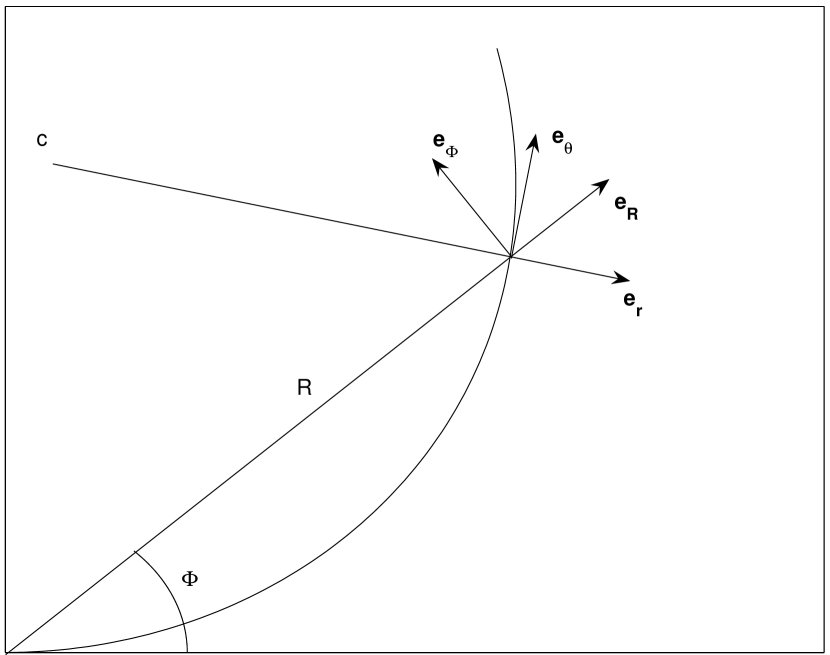
Figure 2: The arm of Archimedes spiral in polar coordinates ($\Phi,R$). Two orthonormal bases are considered: i) polar components of unit vectors, (${\bf e}_{\Phi},{\bf e}_{R}$); and ii) normal and tangential components of unit vectors, (${\bf e}_{r},{\bf e}_{\theta}$), respectively. $C$ is the center of the curvature.

3 Kinematics of particles moving along the curved magnetic field lines

We describe the kinematics of particles moving along the corotating curved magnetic field lines. In particular, we adopt the Archimedes’ spiral for the configuration of magnetic field lines

$$\Phi=aR,$$ (24)

where $\Phi$ and $R$ are the polar coordinates and $a={\it const}$ (see Fig. 2). Rogava et al. (2003) showed that the dynamics of the particle motion asymptotically tends to the force-free regime, if the particle slides along the rotating channel that has the shape of the Archimedes’ spiral. However, in the laboratory frame (LF), the particle follows straight linear paths with constant velocities. In this case, an observer from the LF will measure the effective angular velocity

$$\Omega_{ef}=\Omega+\frac{d\Phi}{dt}=\Omega+av,$$ (25)

where $v$ is the radial velocity of a particle motion, and $\Omega$ is the angular velocity of rotation. If the particle moves without acceleration in the LF, the corresponding effective angular velocity must be equal to zero ($\Omega_{eff}=0$). In this case, Eq. (25) infers that

$$v=v_{c}\equiv-\frac{\Omega}{a},$$ (26)

which means that, for any Archimedes’ spiral with $a<-\Omega/c$, the LF trajectory of the particle becomes a straight line if it moves with a certain ”characteristic velocity”, $v_{c}$.
The relativistic momentum of the particle is given by

$$P_{R}=\gamma mv,$$ (27)

$$P_{\Phi}=\gamma mR\Omega_{ef}\,,$$ (28)

where $m$ and $\gamma$ are the rest mass and the Lorentz factor of the particle, respectively. The expansion of the equation of motion, $d{\bf P}/dt={\bf F}$ (${\bf F}$ is the reaction force), in terms of the radial component

$$F_{R}=-{{aR}\over{\sqrt{1+a^{2}R^{2}}}}|{\bf F}|,$$ (29)

and the angular component

$$F_{\Phi}={{1}\over{\sqrt{1+a^{2}R^{2}}}}|{\bf F}|,$$ (30)

of the reaction force, yields the equation (Rogava et al. (2003))

$$\frac{d^{2}R}{dt^{2}}=\frac{\Omega-\gamma^{2}v(a+\Omega v/c^{2})}{\gamma^{2}\kappa^{2}}\Omega_{ef}R,$$ (31)

where

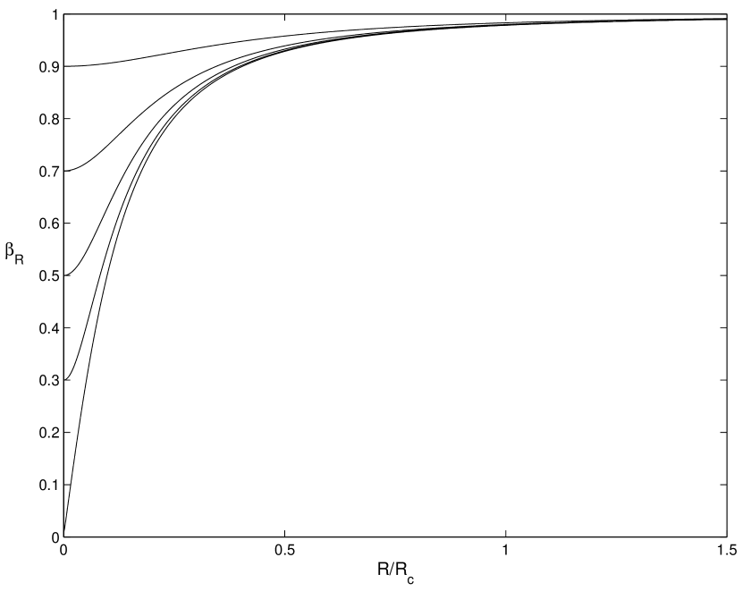
Figure 3: Behaviour of $\beta_{R}$ versus $R/R_{c}$. The set of parameters is $P=1s$, $\beta_{R0}=\{0.01;0.3;0.5;0.7;0.9\}$.

$$\kappa\equiv\left(1-\frac{\Omega^{2}R^{2}}{c^{2}}+a^{2}R^{2}\right)^{1/2}.$$

We note that $(d^{2}R/dt^{2})\equiv 0$, when $v=v_{c}=-\Omega/a$.

Since we are interested in relativistic flows, let us consider $v_{c}=c$ setting $a=-\Omega/c$. In Fig. 3, we plot the solution to Eq. (31), that is the dependence of $\beta_{R}\equiv v/c$ versus $R/R_{c}$ ($R_{c}$ is the light cylinder radius) for the different initial values of $\beta_{R0}$. As is clear from these plots, even though the initial velocity of particles is weakly relativistic (e.g., $\beta_{R0}=0.01$), it asymptotically converges to the characteristic velocity, $v_{c}$. As a result, the particle trajectory in the LF must become linear.

Indeed, in Fig. 4, we show the particle trajectory in the Rotational Frame (RF) of reference (see Fig. 4a) as well as in the LF (see Fig. 4b) for both $\beta_{R0}=0.01$ and the same spiral configuration with $a=-\Omega/c$. Observing the particle trajectory from the LF, one can note that the path asymptotically becomes linear, indicating that the rotational energy pumping process diminishes. Therefore, we conclude that the magnetic field with the of the Archimedes’ spiral may guarantee the saturation process of the CDI.

On the other hand, the equation of Archimedes’ spiral yields $\tan\chi=aR=B_{r}/B_{\theta}$ (see Fig. 1b), resulting in $B_{r}=B_{\theta}$ at the LC when $a=-\Omega/c$.

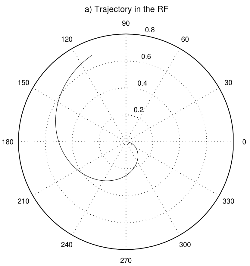
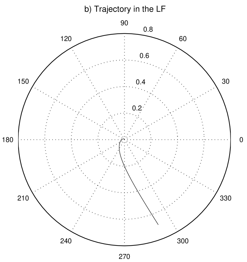
Figure 4: $a$) The trajectory of a particle in the Rotational Frame (RF) of reference; and $b$) the trajectory of a particle in the Laboratory Frame (LF) of reference. The set of parameters is $P=1s$ and $\beta_{R0}^{1}=0.01$. The radial distances are taken in terms of the light cylinder radius, $R/R_{c}$. The trajectory of the particle in RF follows the Archimedes’ spiral ($a$), while the trajectory in the LF asymptotically tends to a straight line configuration ($b$).

4 Discussion

We consider Eq. (23) and plot the timescale of the instability versus the wavelength, $\lambda_{x}$, for several values of initial toroidal perturbations $B^{0}_{r}$. In Fig. 5, we display the behavior of $T(\lambda_{x})$, when $\tan\chi=1$, for several values of initial perturbation $B^{0}_{r}/B_{\theta}\equiv\delta\in\{10^{-1};10^{-3};10^{-5};10^{-7}\}$. Two major applications are examined: (a) 1-second pulsar and (b) the Crab pulsar. From Eq. (23), we can infer that the timescale is a continuously decreasing function of the initial perturbation, $B^{0}_{r}$: as becomes smaller the $\delta$ parameter, so does the initial perturbation and, consequently, the magnetic field lines need more time to achieve the required structure. As observations show, the ratio $P/\dot{P}$ ranges from $10^{11}s$ (PSR 0531 - Crab pulsar) to $10^{18}s$ (PSR 1952+29). However, the greatest values of the twisting timescales, shown in Fig. 5, vary between $10^{4}s$ and $10^{2}s$, which are shorter by many orders of magnitude than $P/\dot{P}$, illustrating the high efficiency of the instability.

The reconstruction of the magnetic field requires a certain amount of energy, therefore it is essential to estimate pulsar’s slowdown luminosity ($L_{p}$) and compare it to the, so-called, ”magnetic luminosity” ($L_{m}\equiv\triangle E_{m}/T$, where $\triangle E_{m}$ is the variation in the magnetic field energy due to the instability). For $L_{p}$, one has

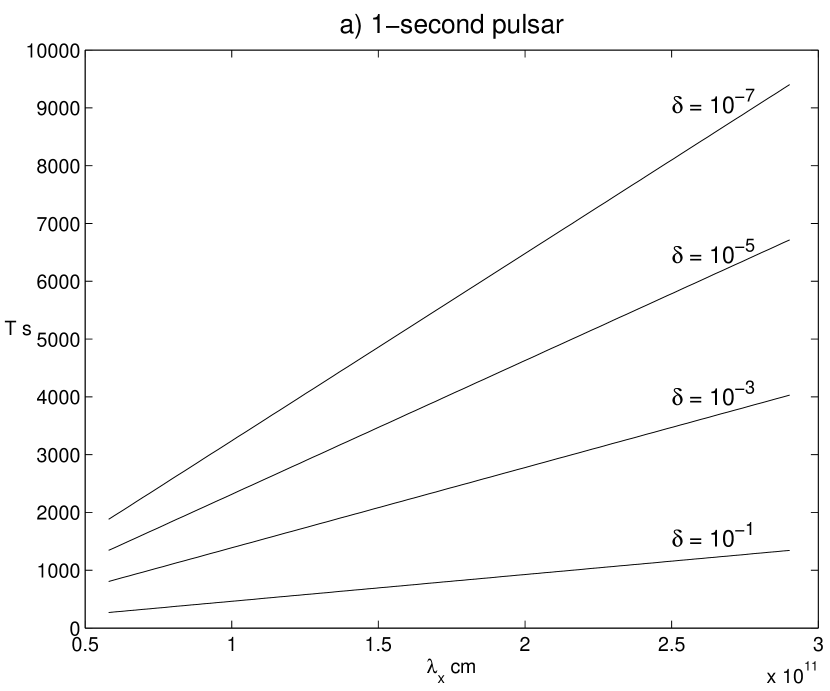
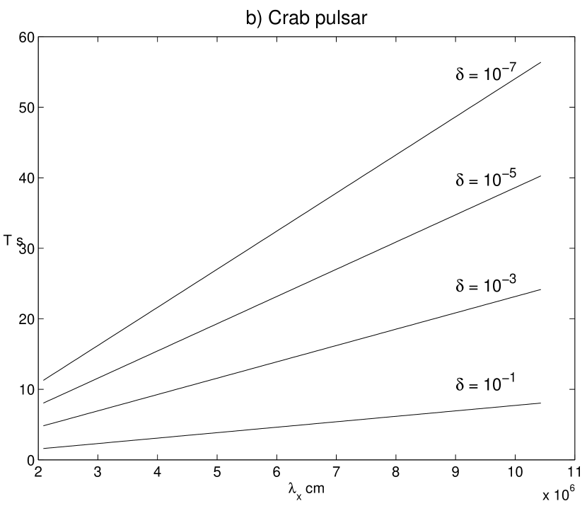
Figure 5: Here we show the behaviour of the timescale of sweepback of the magnetic field lines versus the wave length, $\lambda\approx\lambda_{x}$, for the 1-second pulsar [see (a)] and for the Crab pulsar, $P\approx 0.033s$ [see (b)], respectively. The set of parameters is: $\delta=\{10^{-1};10^{-3};10^{-5};10^{-7}\}$, $\gamma_{b}\sim 10^{6}$ and $\lambda_{\theta}=1000R_{c}$.

$$L_{p}=I\Omega\dot{\Omega}=I\frac{4\pi^{2}}{P^{2}}\frac{\dot{P}}{P},$$ (32)

where $I\sim MR_{p}^{2}$ is the moment of inertia of the pulsar, and $M\sim M_{\odot}\approx 2\times 10^{33}g$ and $R_{p}\sim 10^{6}cm$ are the pulsar’s mass and radius, respectively. For typical pulsars, $\dot{P}/P\sim 10^{-15}s^{-1}$, the slowdown luminosity is estimated to be

$$L_{p}\approx 7.9\times 10^{31}erg/s.$$ (33)

The ”magnetic luminosity”, $L_{m}$, can be estimated straightforwardly

$$L_{m}=\frac{B_{r}^{2}}{4\pi T}\triangle V,$$ (34)

where $\triangle V\sim R_{c}^{2}\triangle r=R_{c}^{3}\varepsilon$ ($\varepsilon\equiv\triangle r/R_{c}<<1$) is the volume, where the process of twisting takes place. Since we are studying the instability in the nearby zone of the LC, the magnetic field components must be given as $B^{0}_{r}\sim\delta\cdot B_{\theta}=\delta\cdot B_{p}(R_{p}/R_{c})^{3}$, where $B_{p}\sim 10^{12}G$ is the magnetic field near the pulsar’s surface. Substituting all quantities into Eq. (34) corresponding to the energy gain for $\lambda_{x}\sim 2.5\times 10^{11}cm$, and $T\approx 10^{3}s$, (see Fig. 5a), and bearing in mind Eqs. (2,23), one can show that for $\varepsilon\sim 0.1$ and $\delta\sim 0.1$ the value of the ”magnetic luminosity” is approximately equal to

$$L_{m}\approx 7.3\times 10^{25}erg/s.$$ (35)

A direct comparison between Eqs. (33) and (35) infers that $L_{m}<<L_{p}$, meaning that approximately only $0.0001\%$ of the total energy budget goes to the reconstruction of the magnetic field lines.

In Fig. 5b, we show the behavior in $T(\lambda_{x})$ for the Crab pulsar in the different cases of initial magnetic perturbations. The dependence does not change qualitatively but the twisting process changes quantitatively as the corresponding timescale is now of the order of $\sim 10\d{-}10^{2}\,s$. The ”magnetic luminosity” of the Crab pulsar for $\delta=0.1$, $\lambda_{x}=7\times 10^{6}cm$, $T\approx 4\,s$ (see Fig. 5b), and $\varepsilon=0.1$ approximately equals [see Eq. (34)]

$$L_{m}^{Crab}\approx 4.7\times 10^{32}erg/s.$$ (36)

On the other hand, a direct calculation of the Crab pulsar ($P\approx 0.033\,s$) luminosity, estimated by Eq. (32), yields

$$L_{p}^{Crab}\approx 9.3\times 10^{38}erg/s.$$ (37)

Therefore, as in the case of the Crab pulsar, the energy required to reconstruct the magnetosphere averages $\sim 0.00005\%$ of the pulsar’s energy and the twisting process becomes feasible in this case as well.

The sweepback mechanism described in this paper, therefore, appears to be extremely efficient for pulsar magnetospheres. The curvature drift instability may lead to the reconstruction of the magnetic field lines in such a way that the dynamics of magnetosphere becomes force-free, which in its turn, completely disrupts the instability, thus saturating the CDI.

5 Summary

We have analytically examined the non-stationary pattern of the pulsar magnetosphere near the LC zone. The GJ current can be estimated by $J_{GJ}=en_{b}c$, giving the value of the corresponding magnetic field, $B_{r}\approx 4\pi J_{GJ}R_{n}/c$, where $R_{n}\approx B(R)/B^{\prime}(R)=R/3$ (where $B^{\prime}\equiv dB/dR$) is the length scale of the spatial inhomogeneity of the magnetic field. If we assume a dipolar configuration, then, taking the value of the GJ density, $n_{b}\approx\Omega B/(2\pi ec)$, into account, one can show that the toroidal magnetic field equals $\frac{2R}{3R_{c}}B$. Inside the light cylinder ($R<R_{c}$), this value is less than the required one-$B$ and reaches its maximum value, $\frac{2}{3}B$, on the light surface. Therefore, the GJ current cannot significantly change the configuration of the magnetic field. This current evidently exceeds the curvature drift current, because $J_{GJ}/J_{cur}\approx c/u_{b}\gg 1$. However, the drift current, $J_{cur}$, is not the source of the toroidal component, $B_{r}$, of the magnetic field, but it is a trigger mechanism for generation of the perturbed current, $J_{1}=e(n_{b}^{0}v^{1}_{b_{x}}+n_{b}^{1}u_{b})$ responsible for the creation of $B_{r}$ (see Eq. (10)). The source of the instability of the current and the resulting magnetic field is the pulsar’s rotational energy. We have found that the instability is achieved by the parametric mechanism, which effectively pumps the pulsar rotational energy directly into the generated mode. The process lasts until the plasma dynamics reaches the force-free regime of motion and the overall magnetosphere relaxes to the steady state configuration. Bucciantini et al. (2006) considered the dynamics of rotating pulsar winds by performing the numerical solution of relativistic magnetohydrodynamic (RMHD) equations in the Schwarzschild metric. The system was allowed to relax to a steady state configuration rapidly approaching the force-free regime. We suppose that the full set of RMHD equations comprises the terms applicable to CDI. Therefore, we highlight the numerical results obtained by Bucciantini et al. (2006) as confirmation of our theory. On the other hand, the aim of the present work was to explain the saturation of the CDI in terms of the generation of currents, which makes the physics of the process more transparent.

The main aspects of the present work can be summarized as follows:

1. Examining the pulsar magnetospheric relativistic plasma, we have studied the role of the parametrically excited CDI in the process of sweepback of magnetic field lines and the saturation process of the instability. The present parametric instability is based on the method developed by Silin (1973), but differs from this in principal, since we study an alternating centrifugal force instead of an alternating electric force.

2. The linear analysis of the Euler, continuity, and induction equations yields the dispersion relation governing the CDI.

3. Considering the resonance frequencies of the sweepback process, an expression of the instability increment has been obtained.

4. On the basis of the expression of the instability growth rate, we have derived the formula of the transition timescale of quasi-linear configuration of field lines into the Archimedes’ spiral. The particles’ motion is force-free along these magnetic field lines, leading to the saturation of the instability.

5. The transition timescale has been compared to the wavelength for 1-second pulsars and the Crab pulsar. For both cases it was shown that the corresponding timescale is shorter than pulsar’s spin down rates by many orders of magnitude illustrating the high efficiency of the discussed process.

References

- Abramovitz & Stegan (1965) Abramovitz, M. & Stegan, I., 1965, Handbook of Mathematical Functions, (eds.: Dover Publications Inc.: New York), p. 320
- Bucciantini et al. (2006) Bucciantini N., Thompson T.A., Arons J., Quataert E. & Del Zanna L., 2006, MNRAS, 368, 1717
- Galeev & Sagdeev (1973) Galeev & Sagdeev, 1973, Nucl. Fussion, 13, 603
- Goldreich & Julian (1969) Goldreich, P. & Julian, W.H., 1969, ApJ, 157, 869
- Kazbegi et al. (1989) Kazbegi A.Z., Machabeli G.Z. & Melikidze G.I., in Joint Varenna-Abastumani International School & Workshop on Plasma Astrophysics, volume ESA SP-285, edited by T.D. Guyenne, (European Space Agency, Paris, 1989), p. 277
- (6) Kazbegi A.Z., Machabeli G.Z. & Melikidze G.I., 1991a, MNRAS, 253, 377
- (7) Kazbegi A.Z., Machabeli G.Z. & Melikidze G.I., 1991b, Aust. J. Phys. 44, 573
- Machabeli et al. (2000) Machabeli G.Z., Mchedlishvili G.Z., & Shapakidze D.E., 2000, Ap&SS, 271, 277
- Machabeli et al. (2005) Machabeli G., Osmanov Z. & Mahajan S., 2005, Phys. Plasmas 12, 062901
- Machabeli & Rogava (1994) Machabeli, G.Z. & Rogava, A. D., 1994, Phys.Rev. A, 50, 98
- Manchester & Taylor (1977) Manchester R. N. & Taylor J. H., 1977, Pulsars (ed.: W. H. Freeman and Company: San Francisco)
- Max (1973) Max C., 1973, Phys. Fluids, 16, 1480
- (13) Mestel L. & Shibata S., 1994, MNRAS, 271, 621
- Osmanov et al. (2008) Osmanov, Z., Dalakishvili, Z. & Machabeli, Z. 2008, MNRAS, 383, 1007
- Piddington (1957) Piddington J.H., 1957, AuJPh, 10, 530
- Rogava et al. (2003) Rogava, A. D., Dalakishvili, G. & Osmanov, Z.N., 2003, Gen. Rel. and Grav. 35, 1133
- Shapakidze et. al (2003) Shapakidze, D., Machabeli, G. Melikidze, G., & Khechinashvili, D., 2003, Phys.Rev.E, 67, 026407
- Silin & Tikhonchuk (1970) Silin V.P. & Tikhonchuk V.T., 1970, J. Appl. Mech. Tech. Phys., 11, 922
- Silin (1973) Silin V.P., 1973, ’Parametricheskoe Vozdeistvie izluchenija bol’shoj mosshnosti na plazmu’, Nauka, Moskva
- Weber & Davis (1967) Weber E.J. & Davis L.Jr., 1967, ApJ, 148, 217