Maximum supercurrent in Josephson junctions with alternating critical current density

Abstract

We consider theoretically and numerically magnetic field dependencies of the maximum supercurrent across Josephson tunnel junctions with spatially alternating critical current density. We find that two flux-penetration fields and one-splinter-vortex equilibrium state exist in long junctions.

I Introduction

Studies of periodic or almost periodic Josephson tunnel structures arranged in sequences of interchanging $0\,$- and $\pi\,$- biased Josephson junctions (as shown in Fig. 1) recently became a subject of growing interest. These complex Josephson systems are intensively treated experimentally, theoretically, and numerically in: (a) superconductor-ferromagnet-superconductor (SFS) junctions in thin filmsBulaevskii et al. (1977); Buzdin et al. (1982); Ryazanov et al. (2001); Kontos et al. (2002); Blum et al. (2002) and (b) Josephson grain boundaries in thin films of high-temperature cooper-oxide superconductor YBa₂Cu₃O_7-x.Buchal et al. (1995); Hilgenkamp et al. (1996); Van Harlingen (1995); Tsuei and Kirtley (2000); Hilgenkamp and Mannhart (2002); Mannhart et al. (1996); Mints and Kogan (1997); Mints (1998); Mints et al. (2002); Buzdin and Koshelev (2003)

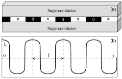
Figure 1: Schematic drawings of: (a) sequence of $0\,$- and $\pi\,$- biased Josephson junctions; (b) critical current density, $j_{c}(x)$.

Equilibrium states of SFS Josephson junctions with a $\pi$-shift in the phase difference between the superconducting banks has been predicted almost three decades ago.Bulaevskii et al. (1977); Buzdin et al. (1982) However, only recently SFS $\pi\,$- shifted junctions and SFS heterostructures of interchanging $0\,$- and $\pi\,$- shifted fragments were studied experimentally for the first time. Ryazanov et al. (2001); Kontos et al. (2002); Blum et al. (2002)

The studies of Josephson properties of the asymmetric grain boundaries in YBa₂Cu₃O_7-x thin films reveal an interesting and important example of a Josephson system being an interchanging sequence of $0\,$-$\pi$ biased junctions.Buchal et al. (1995); Hilgenkamp et al. (1996); Van Harlingen (1995); Tsuei and Kirtley (2000); Hilgenkamp and Mannhart (2002) The structure of these boundaries is created by facets with a variety of orientations and lengths $l\sim 10-100\,$nm.Hilgenkamp and Mannhart (2002) This grain boundary structure in conjunction with the $d_{x^{2}-y^{2}}$-wave symmetry of the order parameterVan Harlingen (1995); Tsuei and Kirtley (2000) can be considered as a Josephson tunnel junction with spatially alternating critical current density, $j_{c}(x)$, where $x$ axis is along the grain boundary.Van Harlingen (1995); Tsuei and Kirtley (2000); Hilgenkamp and Mannhart (2002) These rapid alternations with a typical length-scale of $l$ significantly suppress the maximum supercurrent $I_{\rm m}$ across the grain boundaries. This suppression is most effective for the asymmetric 45^∘ [001]-tilt grain boundaries in YBa₂Cu₃O_7-x films.Hilgenkamp et al. (1996); Hilgenkamp and Mannhart (2002)

The asymmetric 45^∘ [001]-tilt grain boundaries in thin YBa₂Cu₃O_7-x films exhibit several remarkable and important anomalies. First, the dependence of the maximum supercurrent $I_{\rm m}$ on the applied magnetic field $H_{a}$ is non-Fraunhofer.Buchal et al. (1995); Hilgenkamp et al. (1996); Mints and Kogan (1997); Buzdin and Koshelev (2003) Contrary to the classical Fraunhofer pattern with the central major peak two symmetric major side-peaks appear at the two fields $\pm\,H_{\rm sp}\neq 0$. Second, a spontaneous rapidly alternating magnetic flux is generated at the grain boundaries.Mannhart et al. (1996) Third, unquantized spontaneous flux structures include fragments formed by pairs of single Josephson-type vortices carrying fluxes $\phi_{1}<\phi_{0}/2$ and $\phi_{2}>\phi_{0}/2$. Mints (1998); Mints et al. (2002) These fluxes are complimentary and sum to $\phi_{0}$, i.e., $\phi_{1}+\phi_{2}=\phi_{0}$ and therefore introduce splintered Josephson vortices. It is worth noting here that the anomalous patterns $I_{m}(H_{a})$ and the unquantized splinter vortices appear under conditions of existence of equilibrium spontaneous flux.

In many cases the length-scale $l$ of the spatial alternations of the critical current density $j_{c}(x)$ is bigger or much bigger than the London penetration depth, $\lambda$, and is smaller or much smaller than the local Josephson penetration depth, $\lambda_{J}$, defined by the average of the absolute value of the critical current density. In the limit of $l\ll\lambda_{J}$ the phase difference between the banks of the tunnel junction, $\varphi(x)$, can be written as a sum of smooth, $\psi(x)$, and rapidly varying, $\xi(x)$, terms.Mints (1998) Coarse-graining the phase $\varphi(x)$ over a distance ${\cal L}\gg l$ allows to consider the two terms $\psi(x)$ and $\xi(x)$ separately from each other in the inner part of the junction. In this approximation the coupling of $\psi(x)$ and $\xi(x)$ happens because of the boundary conditions at the edges of the junction.

In this paper we calculate both theoretically and numerically the anomalous magnetic field dependence of the maximum supercurrent, $I_{m}$, in Josephson tunnel junctions with spatially alternating critical current density. The applied magnetic field $H_{a}$ is supposed to be lower than the side-peaks field, i.e., $|H_{a}|\ll H_{\rm sp}\sim\phi_{0}/2\pi\lambda\,l$.

The paper is organized as follows. In Sec. II we discuss the coarse-grained equations for the phase difference across the banks of Josephson junctions with alternating critical current density and derive the boundary conditions to these equations. In Sec. III we consider the maximum supercurrent across Josephson junctions theoretically in two limiting cases of short and long junctions in low and high magnetic fields. In Sec. IV we report on the results of numerical simulations of the maximum supercurrent dependence on the applied magnetic field. Sec. VII summarizes the overall conclusions.

II Coarse-grained equations

We treat a one-dimensional Josephson junction parallel to the $x$ axis with the tunneling current density ${\bf j}\,\|\,\hat{\bf y}$, $j_{y}(x)=j(x)$, and the magnetic field ${\bf H}\,\|\,\hat{\bf z}$, $H_{z}(x)=H(x)$. Assume also that the critical current density $j_{c}(x)$ is an alternating periodic or almost periodic function taking positive and negative values with a typical length-scale $l$. The geometry of the problem is shown schematically in Fig. 1.

First, we introduce the average value of the critical current density, $\langle\,j_{c}\rangle$, the effective Josephson penetration depth, $\Lambda$, defined by $\langle\,j_{c}\rangle$, and the local Josephson penetration depth, $\lambda_{J}$, defined by the average value of $|j_{c}|$

$$\langle\,f\rangle = {1\over L}\int_{0}^{L}f(x)\,dx\,,$$ (1)

$$\Lambda = \sqrt{c\phi_{0}\over 16\pi^{2}\lambda\,\langle\,j_{c}\rangle}\,,$$ (2)

$$\lambda_{J} = \sqrt{c\phi_{0}\over 16\pi^{2}\lambda\langle\,|j_{c}|\rangle}\,,$$ (3)

where Eq. (1) is the definition of averaging, $L$ is the length of the junction ($L\gg l$), $\phi_{0}$ is the flux quantum, and $\lambda$ is the London penetration depth.

Next, we assume that $\lambda\ll l\ll\lambda_{J}\ll\Lambda$. In this case the phase difference $\varphi(x)$ satisfies the equation

$$\Lambda^{2}\varphi^{\prime\prime}-{j_{c}(x)\over\langle j_{c}\rangle}\,\sin\varphi=0.$$ (4)

It is convenient for the following analyses to write the critical current density $j_{c}(x)$ in the form

$$j_{c}(x)=\langle j_{c}\rangle\,[1+g(x)]$$ (5)

introducing a rapidly alternating function $g(x)$ with a zero average value, $\langle g(x)\rangle=0$, and a typical length-scale of order $l$. It is worth noting that $g(x)$ is a unique internal characteristic of a junction. Using the function $g(x)$ we rewrite Eq. (4) as

$$\Lambda^{2}\varphi^{\prime\prime}-[1+g(x)]\,\sin\varphi=0\,.$$ (6)

The idea of the following calculation is based on a mechanical analogy (Kapitza’s pendulum).Landau and Lifshitz (1976); Arnold and Neishtadt (1997) Two types of terms appear in Eq. (6): fast terms alternating over a length $l$ and smooth terms varying over a length $\Lambda\gg l$. The fast alternating terms cancel each other, independently of the smooth terms, which also cancel each other.

Thus, to find solutions of Eq. (6) we use the ansatz

$$\varphi(x)=\psi(x)+\xi(x)\,,$$ (7)

where $\psi(x)$ is a smooth function with the length-scale of order $\Lambda$, $\xi(x)$ is a rapidly alternating function with the length-scale of order $l$, and the variations of $\xi(x)$ are small, i.e., $\langle|\xi(x)|\rangle\ll 1$.Mints (1998) We assume also that the average value of $\xi(x)$ is zero, $\langle\xi(x)\rangle=0$. It is worth mentioning that the ansatz given by Eq. (7) is similar to the one used to solve the Kapitza’s pendulum.Landau and Lifshitz (1976); Arnold and Neishtadt (1997)

Substituting Eq. (7) into Eq. (6) and keeping terms up to first order in $\xi(x)$ we find Mints (1998)

$$\Lambda^{2}\psi^{\prime\prime}-{j_{\psi}(x)\over\langle j_{c}\rangle} = 0\,,$$ (8)

$$\Lambda^{2}\xi^{\prime\prime}-{j_{\xi}(x)\over\langle j_{c}\rangle} = 0\,,$$ (9)

where the smooth $j_{\psi}(x)$ and alternating $j_{\xi}(x)$ components of the tunneling current density $j=j_{\psi}+j_{\xi}$ are

$$j_{\psi} = \langle j_{c}\rangle\left(\sin\psi-\gamma\sin\psi\cos\psi\right)\,,$$ (10)

$$j_{\xi} = \langle j_{c}\rangle\,g(x)\sin\psi\,,$$ (11)

the dimensionless constant $\gamma$ is equal to

$$\gamma=\langle g(x)\xi_{g}(x)\rangle\,,$$ (12)

and the rapidly alternating phase $\xi_{g}(x)$ is defined by

$$\xi(x)=-\xi_{g}(x)\sin\psi\,.$$ (13)

It follows from Eqs. (9), (11) and (13) that

$$\Lambda^{2}\xi^{\prime\prime}_{g}+g(x)=0\,,$$ (14)

i.e., the rapidly alternating phase shift $\xi_{g}$ depends only on the effective penetration depth $\Lambda$ and the function $g(x)$. Therefore, the phase $\xi_{g}(x)$ is an internal characteristics of a junction.

It follows from Eq. (10) that the smooth current density $j_{\psi}$ includes the initial first harmonic term $\propto\sin\psi$ and an additional second harmonic term $\propto\sin 2\psi$, which results from constructive interference of the rapidly alternating critical current density $\propto g(x)$ and phase $\xi(x)$. Mints (1998)

To summarize the derivation of the system of coarse-grained equations (8)–(11) it is worth noting that the typical value of $\xi_{g}(x)$ is small, but at the same time the typical value of $g(x)$ is big, i.e., $\langle|\xi_{g}(x)|\rangle\ll 1$ and $\langle|g(x)|\rangle\gg 1$. As a result, the dimensionless parameter $\gamma$, which is proportional to the average of the product of the two rapidly alternating functions $\xi_{g}(x)$ and $g(x)$ might be of the order of unity.Mints (1998); Mints et al. (2002)

The energy ${\cal E}$ of a junction with alternating critical current density $j_{c}(x)$ yields

$${\cal E}={\hbar\langle j_{c}\rangle\over 2e}\int_{0}^{L}\!\!\left({\Lambda^{2}\over 2}\,\psi^{\prime 2}+1-\cos\psi-{\gamma\over 2}\sin^{2}\psi\right)dx.$$ (15)

The last term in the integral in Eq. (15) is for the contribution of both the fast alternating current $j_{\xi}(x)$ and phase $\xi(x)$. It is worth noting that minimization of the functional ${\cal E}\{\psi\}$ results in Eq. (8) for the phase $\psi(x)$.

It follows from Eqs. (8) and (15) that if the parameter $\gamma>1$, then there are two series of stable uniform equilibrium states with $\psi_{e}=2\pi n\pm\psi_{\gamma}$ and current density $j_{\psi}(\psi_{e})=0$, where $n=0,\pm 1,\pm 2,\,\dots$ is an integer and the phase $\psi_{\gamma}$ is defined byMints (1998)

$$\gamma\cos\psi_{\gamma}=1\,.$$ (16)

All equilibrium states with $\psi=\psi_{e}$ have the same energy

$${\cal E}_{\gamma}=-{\hbar\langle j_{c}\rangle\over 2e}\,{(\gamma-1)^{2}\over 2\gamma}\,L\,,$$ (17)

which is less then the energy ${\cal E}_{0}=0$ of the series of unstable states with the phase $\psi=2\pi n$.Mints (1998) If the parameter $\gamma<1$, then there is only one series of stable uniform equilibrium states with $\psi_{0}=2\pi n$ and ${\cal E}_{0}=0$.

The two series of stable equilibrium states result in existence of two different single Josephson vortices (two splinters).Mints (1998); Mints et al. (2002) The phase $\psi(x)$ for the first (“small”) splinter vortex varies from $-\psi_{\gamma}$ at $x=-\infty$ to $\psi_{\gamma}$ at $x=+\infty$. This vortex carries flux $\phi_{1}=\phi_{0}\psi_{\gamma}/\pi\leq\phi_{0}/2$. The phase for the second (“big”) splinter vortex varies from $\psi_{\gamma}$ at $x=-\infty$ to $2\pi-\psi_{\gamma}$ at $x=\infty$. This vortex caries flux $\phi_{2}=\phi_{0}(\pi-\psi_{\gamma})/\pi\geq\phi_{0}/2$. As a result any flux structure inside a junction with an alternating critical current density and with $\gamma>1$ consists of series of interchanging small and big splinter vortices. Mints (1998); Mints et al. (2002) It is also important mentioning that $\phi_{1}+\phi_{2}=\phi_{0}$.

Consider now the boundary conditions to Eq. (8), i.e., for the smooth phase shift $\psi(x)$. Using equations

$$H = {\phi_{0}\over 4\pi\lambda}\,{d\varphi\over dx}\,,$$ (18)

$$\varphi(x) = \psi(x)-\xi_{g}(x)\,\sin\psi(x)$$ (19)

we find the boundary conditions for $\psi(x)$ in the form

$$\varphi^{\prime}(0) = \psi^{\prime}_{0}-\xi^{\prime}_{\rm g0}\sin\psi_{0}={4\pi\lambda\over\phi_{0}}\,H_{0}\,,$$ (20)

$$\varphi^{\prime}(L) = \psi^{\prime}_{L}-\xi^{\prime}_{\rm gL}\sin\psi_{L}={4\pi\lambda\over\phi_{0}}\,H_{L}\,,$$ (21)

where $\psi_{0}=\psi(0)$, $\psi_{L}=\psi(L)$, $\psi^{\prime}_{0}=\psi^{\prime}(0)$, $\psi^{\prime}_{L}=\psi^{\prime}(L)$, $H_{0}=H(0)$, $H_{L}=H(L)$, $\xi^{\prime}_{\rm g0}=\xi_{g}^{\prime}(0)$, and $\xi^{\prime}_{\rm gL}=\xi^{\prime}_{g}(L)$. Next, we use the fact that the average value of $g(x)$ is zero and integrate Eq. (14) from $0$ to $L$. This leads to

$$\xi^{\prime}_{\rm g0}=\xi^{\prime}_{\rm gL}=\xi^{\prime}_{\rm gb},$$ (22)

where $\xi^{\prime}_{\rm gb}$ is an internal parameter characterizing the edges of the junction. Now the boundary conditions given by Eqs. (20) and (21) take the form

$$\psi^{\prime}_{0}-\xi^{\prime}_{\rm gb}\sin\psi_{0} = {4\pi\lambda\over\phi_{0}}\,H_{0}\,,$$ (23)

$$\psi^{\prime}_{L}-\xi^{\prime}_{\rm gb}\sin\psi_{L} = {4\pi\lambda\over\Phi_{0}}\,H_{L}\,.$$ (24)

Compare now the values of the derivatives $\psi_{0}^{\prime}$, $\psi^{\prime}_{L}$, and $\xi^{\prime}_{\rm gb}$. Using Eqs. (9), (12) and (14) we obtain

$$\gamma=\langle g(x)\,\xi_{g}\rangle=-\langle\Lambda^{2}\xi^{\prime\prime}_{g}(x)\xi_{g}(x)\rangle=\langle\left[\Lambda\xi_{g}^{\prime}(x)\right]^{2}\rangle$$ (25)

and arrive to the relation

$$\Lambda\,|\xi_{g}^{\prime}(x)|\sim\sqrt{\gamma}\sim 1.$$ (26)

A similar estimate $\Lambda|\psi^{\prime}(x)|\sim 1$ follows from Eqs. (8) and (10). These estimates demonstrate that both derivatives $\psi^{\prime}(x)$ and $\xi^{\prime}_{g}(x)$ are of the same order although $\langle|\xi_{g}(x)|\rangle\ll\langle|\psi(x)|\rangle$. Indeed, for a typical junction exhibiting spontaneous equilibrium flux we have $\gamma\sim 1$.Mints et al. (2002)

The fact that $\Lambda\xi^{\prime}_{\rm gb}\sim 1$ makes it convenient for the following analysis to write the derivative $\xi^{\prime}_{\rm gb}$ in the form

$$\xi^{\prime}_{\rm gb}={\alpha\over\Lambda},$$ (27)

where $\alpha\sim 1$ is an internal parameter characterizing the edges of the junction.

Thus, in the framework of the coarse-grained approach a junction with an alternating critical current density is characterized by two dimensionless parameters $\alpha$ and $\gamma$.

Assume, that the current across a junction $I\neq 0$, then we have the relations

$$H_{0}=H_{a}+{2\pi\over c}I\,,$$ (28)

$$H_{L}=H_{a}-{2\pi\over c}I.$$ (29)

In this case the boundary conditions given by Eqs. (23) and (24) take the final form

$$\psi^{\prime}_{0}={4\pi\lambda\over\phi_{0}}\,H_{a}+{8\pi^{2}\lambda\over c\phi_{0}}\,I+{\alpha\over\Lambda}\sin\psi_{0}\,,$$ (30)

$$\psi^{\prime}_{L}={4\pi\lambda\over\phi_{0}}\,H_{a}-{8\pi^{2}\lambda\over c\phi_{0}}\,I+{\alpha\over\Lambda}\sin\psi_{L}\,.$$ (31)

The fact that the rapidly alternating critical current density $j_{c}(x)$ has low average value $[\langle j_{c}(x)\rangle\ll\langle|j_{c}(x)|\rangle]$ might significantly affect the maximum supercurrent. Indeed, assume that the Josephson current density includes both the first and the second harmonics,Golubov et al. (2004) i.e.,

$$j=j_{\rm c1}(x)\sin\varphi+j_{\rm c2}\sin 2\varphi\,,$$ (32)

where $j_{\rm c1}(x)$ is rapidly alternating along the junction and $j_{\rm c2}$ is spatially independent.

In this case the coarse-graining approach remains the same as above. The effect of the second harmonics on the maximum supercurrent $I_{m}$ increases with the increase of the dimensionless parameter $\gamma_{2}=j_{\rm c2}/\langle j_{\rm c1}\rangle$. The value of $\gamma_{2}$ might be of order of unity and higher even if $j_{\rm c2}$ is low compared to $\langle|j_{\rm c1}(x)|\rangle$.

III Maximum Supercurrent

The Josephson tunneling current, $I$, across Josephson tunnel junction with an alternating critical current density can be written as a sum of two terms $I_{\psi}$ and $I_{\xi}$

$$I=\int_{0}^{L}j\,dx=I_{\psi}+I_{\xi}\,,$$ (33)

where the currents $I_{\psi}$ and $I_{\xi}$ are given by

$$I_{\psi} = \int_{0}^{L}j_{\psi}\,dx=I_{c}\,\Lambda\left(\psi^{\prime}_{L}-\psi^{\prime}_{0}\right)\,,$$ (34)

$$I_{\xi} = \int_{0}^{L}j_{\xi}\,dx=\alpha I_{c}\,(\sin\psi_{0}-\sin\psi_{L})\,,$$ (35)

and the current $I_{c}$ is defined as

$$I_{c}=\Lambda\langle j_{c}\rangle\,.$$ (36)

It follows from Eqs. (34) and (35) that both $I_{\psi}$ and $I_{\xi}$ are defined by the smooth phase $\psi$ only.

Magnetic flux inside the junction

$$\phi=2\lambda\,\int_{0}^{L}H\,dx={\phi_{0}\over 2\pi}\,(\psi_{L}-\psi_{0})$$ (37)

results in the phase difference

$$\psi_{L}-\psi_{0}=2\pi\,{\phi\over\phi_{0}}\,.$$ (38)

Using Eqs. (35) and (38) we obtain the current $I_{\xi}$ as a function of the flux inside the junction

$$I_{\xi} = \alpha I_{c}\bigg{[}\sin\psi_{0}-\sin\bigg{(}\psi_{0}+2\pi{\phi\over\phi_{0}}\bigg{)}\bigg{]}=$$ (39)

$$= -2\alpha I_{c}\sin\bigg{(}\pi{\phi\over\phi_{0}}\bigg{)}\cos\bigg{(}\psi_{0}+\pi{\phi\over\phi_{0}}\bigg{)}\,.$$

In order to calculate the total current $I_{\psi}$ one has to know the spatial distribution of the phase $\psi(x)$ in detail.

In what follows we calculate the maximum supercurrent $I_{m}$ theoretically in the limiting cases of short $(L\ll\Lambda$) and long ($L\gg\Lambda$) junctions treating the problem separately for the Meissner and mixed states.

III.1 Maximum current across short junctions

We calculate now the maximum supercurrent $I_{m}(H_{a})$ of a short junction, $L\ll\Lambda$. In this case the spatial dependence of the smooth phase $\psi(x)$ in the main approximation in $L/\Lambda\ll 1$ is linear

$$\psi(x)=\psi_{0}+2\pi\,{\phi_{i}\over\phi_{0}}\,{x\over L},$$ (40)

where

$$\phi_{i}=2\lambda LH_{i}$$ (41)

is the “internal” flux and $H_{i}$ is the magnetic field inside the junction. Next, we use Eqs. (30), (31), (34), (35), and (40) and obtain the following relations

$$H_{i} = H_{a},$$ (42)

$$\psi_{L} = \psi_{0}+2\pi\,{\phi_{a}\over\phi_{0}},\quad\phi_{a}=2\lambda LH_{a}\,,$$ (43)

$$I = \alpha I_{c}\,\left(\sin\psi_{L}-\sin\psi_{0}\right)\,.$$ (44)

Combining Eqs. (43) and (44) we find that the maximum value of the total current $I(\phi_{a})$ is given by

$$I_{m}=2\alpha I_{c}\left|\,\sin\left(\pi{\phi_{a}\over\phi_{0}}\right)\right|\,.$$ (45)

It follows from Eq. (45) that the maximum supercurrent across short junctions with spatially alternating critical current density is defined only by the surface current $I_{\xi}$ (in the main approximation in $L/\Lambda\ll 1$). As a result the dependence $I_{m}(\phi_{a})$ is obviously non-Fraunhofer. The value of $I_{m}$ is oscillating periodically in $\phi_{a}$ with the period that is equal to flux quantum $\phi_{0}$. Contrary to the case of a constant critical current density the amplitude of oscillations of $I_{m}$ is not decreasing with the increase of the applied field $H_{a}$.Kulik and Janson (1972); Barone and Paterno (1982)

III.2 Meissner and mixed states in long junctions

In this subsection we consider the spatial distributions of the phase difference and the flux in long junctions, $L\gg\Lambda$. We start with the low field limit, i.e., we assume that the applied field $H_{a}\ll H_{s}$, where

$$H_{s}={\phi_{0}\over 2\pi\lambda\Lambda}$$ (46)

is the flux penetration field for a long junction with a constant critical current density $j_{c}={\rm const}$.Kulik and Janson (1972); Barone and Paterno (1982) In the following analysis we use an approach similar to the one, which was first developed by Owen and Scalapino. Owen and Scalapino (1967)

Figure 2: Spatial distributions of the phase $\psi(x)$ in a long junction for different values of the applied field $H_{a}$ and the internal flux $\phi_{i}$. (a) $H_{a}<H_{\rm s1}$, $\phi_{i}=0$, (b) $H_{\rm s1}\leq H_{a}\leq H_{\rm s2}$, $\phi_{i}=\phi_{1}$, (c) $H_{a}>H_{\rm s2}\,$, $\phi_{i}\approx\phi_{a}$.

In the case of $L\gg\Lambda$ and $H_{a}\ll H_{s}$ the total supercurrent $I=I_{\psi}+I_{\xi}$ is a surface current localized in a layer with a width $\sim l\gg\lambda$. It follows from Eqs. (34) and (35) that in order to calculate $I_{\psi}$ and $I_{\xi}$ we have to find the dependencies of $\psi^{\prime}_{L}$ and $\psi^{\prime}_{0}$ on $\psi_{0}$ and $\psi_{L}$. These dependencies are given by the first integral of Eq. (8)

$${\Lambda^{2}\over 2}\psi^{\prime 2}+\cos\psi-{\gamma\over 4}\cos 2\psi={\rm const}\,.$$ (47)

It is worth mentioning that Eq. (47) describes the density of the energy ${\cal E}$ given by Eq. (15).

The spatial distribution of $\psi(x)$ depends on the magnetic prehistory of the sample. We begin here for brevity with the case of a junction in the Meissner state. In this case the flux is localized at the edges of the junction. As a result in a long junction the phase $\psi(x)$ in the inner part equals to a certain constant $\psi_{\infty}$. The first correction to this constant is proportional to $\exp{(-L/\Lambda)}\ll 1$. In other words we have

$$\psi(L/2)=\psi_{\infty}\,,\quad\psi^{\prime}(L/2)=0\,,$$ (48)

where the phase $\psi_{\infty}$ is given by one of the stable equilibrium values of $\psi$, i.e., $\cos\psi_{\infty}=1/\gamma$. Combining Eqs. (47), (48) and (16) we find that the constant in the RHS of Eq. (47) is given by

$${\rm const}=\cos\psi_{\infty}-{\gamma\over 4}\cos 2\psi_{\infty}={\gamma\over 4}+{1\over 2\gamma}\,.$$ (49)

The above relation allows for transforming Eq. (47) into

$$\Lambda^{2}\psi^{\prime 2}=\gamma\left(\cos\psi_{\gamma}-\cos\psi\right)^{2}.$$ (50)

We calculate first the flux penetration field into a junction with an alternating critical current density and a zero total current, $I=0$. The dependence $\psi(x)$ for this case is shown schematically in Fig. 2 (a). It follows then from Eq. (50) that

$$\Lambda\psi^{\prime}_{0}=\sqrt{\gamma}(\cos\psi_{0}-\cos\psi_{\gamma})\,,$$ (51)

$$\Lambda\psi^{\prime}_{L}=\sqrt{\gamma}(\cos\psi_{\gamma}-\cos\psi_{L})\,.$$ (52)

Next, we combine Eqs. (30), (51), (31), and (52) and obtain two relations between the applied field $H_{a}$ and the phases $\psi_{0}$ and $\psi_{L}$

$$H_{a}={H_{s}\over 2}\,\left[\sqrt{\gamma+\alpha^{2}}\,\cos\left(\psi_{0}+\psi_{\alpha}\right)-{1\over\sqrt{\gamma}}\right]\,,$$ (53)

$$H_{a}={H_{s}\over 2}\,\left[{1\over\sqrt{\gamma}}-\sqrt{\gamma+\alpha^{2}}\,\cos\left(\psi_{L}-\psi_{\alpha}\right)\right]\,.$$ (54)

where we introduce the phase $\psi_{\alpha}$ as

$$\tan\psi_{\alpha}={\alpha\over\sqrt{\gamma}}\,.$$ (55)

In the following analysis we assume, for definiteness, that $\psi_{\alpha}<\psi_{\gamma}$. In this case the dependence $\psi(x)$ looks as shown schematically in Fig. 2.

As a function of $\psi_{0}$ the RHS of Eq. (53) is bounded. The maximum field

$$H_{\rm s1}={H_{s}\over 2}\,\left[\sqrt{\gamma+\alpha^{2}}-{1\over\sqrt{\gamma}}\,\right]$$ (56)

is achieved at

$$\psi_{0}=-\psi_{\alpha}\,.$$ (57)

Therefore, if the applied field $H_{a}$ reaches the value of $H_{\rm s1}$ then the Meissner state in a long junction becomes unstable and the small splinter vortexMints (1998); Mints et al. (2002) carrying flux

$$\phi_{1}=\phi_{0}{\psi_{\gamma}\over\pi}\leq\phi_{0}/2$$ (58)

enters into the inner part of the junction as shown in Fig. 2 (b). This feature is a direct consequence of existence of the splinter vortices in junctions with $\gamma\geq 1$.

It follows from Eq. (50) that in this one-vortex state

$$\Lambda\psi^{\prime}_{\rm 0,L}=\sqrt{\gamma}\left(\cos\psi_{\gamma}-\cos\psi_{\rm 0,L}\right)>0\,.$$ (59)

Using Eqs. (30), (31), and (59) we obtain the relations between the applied field $H_{a}$ and the phases $\psi_{0}$ and $\psi_{L}$

$$H_{a}={H_{s}\over 2}\,\left[{1\over\sqrt{\gamma}}-\sqrt{\gamma+\alpha^{2}}\,\cos\left(\psi_{0}-\psi_{\alpha}\right)\right]\,,$$ (60)

$$H_{a}={H_{s}\over 2}\,\left[{1\over\sqrt{\gamma}}-\sqrt{\gamma+\alpha^{2}}\,\cos\left(\psi_{L}-\psi_{\alpha}\right)\right]\,.$$ (61)

The RHS’s of Eqs. (60) and (61) are bounded as functions of $\psi_{0}$ and $\psi_{L}$ and the maximum field

$$H_{\rm s2}={H_{s}\over 2}\,\left[\sqrt{\gamma+\alpha^{2}}+{1\over\sqrt{\gamma}}\,\right]$$ (62)

is achieved at $\psi_{0}=\psi_{\alpha}-\pi+2\pi n$ and $\psi_{L}=\psi_{\alpha}+\pi+2\pi m$ where $n,m=0,\pm 1,\pm 2,...$ are integers. If the applied field $H_{a}$ reaches the value of $H_{\rm s2}$ the one-vortex state becomes unstable and magnetic flux penetrates into the bulk until a mixed state with a finite density of vortices is established (see Fig. 2 (c)).

Therefore, the rapid spatial alternations of the critical current density $j_{c}(x)$ in case of $\gamma\geq 1$ lead to existence of a specific equilibrium one-splinter-vortex state. This state appear if the applied field $H_{a}$ is from the interval $H_{\rm s1}\leq H_{\rm a}\leq H_{\rm s2}$. It is worth noting here that the case of a standard Josephson junction ($j_{c}={\rm const}$) corresponds to $\alpha=0$ and $\gamma=1$. It follows then from Eqs. (58), (56), (62), and (46) that for these values of the parameters $\alpha$ and $\beta$ we have $\phi_{1}=0$, $\phi_{2}=\phi_{0}$, $H_{\rm s1}=0$, and $H_{\rm s2}=H_{s}$, i.e., there is only one Josephson vortex and the Meissner state exists if $0\leq H_{a}\leq H_{s}$ as it has to be.Kulik and Janson (1972) This verification means that the above results are self-consistent in describing the case of a standard Josephson junction.

III.3 Maximum supercurrent in the Meissner state

We calculate now the maximum supercurrent $I_{m}$ in the Meissner state in a long junction, i.e., we assume that $L\gg\Lambda$ and the smooth phase $\psi$ inside the junction is given by one of its equilibrium values $\psi_{e}=2\pi n\pm\psi_{\gamma}$, where $n=0,\pm 1,\pm 2,...$ is an integer. The spatial distribution of $\psi(x)$ corresponding to the current $I_{m}$ is shown in Fig. 2 (a). It follows then from Eq. (50) that

$$\psi^{\prime}_{0}={\sqrt{\gamma}\over\Lambda}\,(\cos\psi_{\gamma}-\cos\psi_{0}),$$ (63)

$$\psi^{\prime}_{L}={\sqrt{\gamma}\over\Lambda}\,(\cos\psi_{L}-\cos\psi_{\gamma})\,.$$ (64)

Using Eqs. (63), (64) and the boundary conditions given by Eqs. (30) and (31) we obtain equations relating the current $I$, the applied field $H_{a}$ and the phases $\psi_{0}$ and $\psi_{L}$

$$H_{a}={1\over 2}\,H_{m}\left[\cos(\psi_{L}+\psi_{\alpha})-\cos(\psi_{0}-\psi_{\alpha})\right]\,,$$ (65)

$${I\over I_{c}}={2\over\sqrt{\gamma}}-2\,{H_{m}\over H_{s}}\left[\cos(\psi_{0}-\psi_{\alpha})+\cos(\psi_{L}+\psi_{\alpha})\right]\,,$$ (66)

where we introduce the field $H_{m}$ as

$$H_{m}={{H_{\rm s1}+H_{\rm s2}}\over 2}={H_{s}\over 2}\,\sqrt{\gamma+\alpha^{2}}\,.$$ (67)

The two relations given by Eqs. (65) and (66) allow to obtain the dependence of the current $I$ on the field $H_{a}$ and the phase $\psi_{0}$ in the form

$${I\over I_{c}}={2\over\sqrt{\gamma}}-4{H_{a}\over H_{s}}-4\,{H_{m}\over H_{s}}\,\cos(\psi_{0}-\psi_{\alpha})\,.$$ (68)

It follows from Eq. (68) that the maximum current $I_{m}$ corresponds to $\cos(\psi_{0}-\psi_{\alpha})=-1$. Combining the above calculation valid for $H_{a}>0$ with the one valid for $H_{a}<0$ we obtain the dependence $I_{m}(H_{a})$ in its final form

$$I_{m}=4I_{c}\,{{H_{\rm s2}-|H_{a}|}\over H_{s}}={c\over 2\pi}\,(H_{\rm s2}-|H_{a}|)\,.$$ (69)

Thus, in the Meissner state the maximum value of $I_{m}$ is achieved at $H_{a}=0$ and is equal to

$$I_{m}(0)={cH_{\rm s2}\over 2\pi}=2I_{c}\,\left[\sqrt{\gamma+\alpha^{2}}+{1\over\sqrt{\gamma}}\right].$$ (70)

It is worth noting that for a standard Josephson junction ($\alpha=0,\gamma=1$) and therefore we have $H_{\rm s2}=H_{s}$. As a result Eqs. (69) and (70) coincide with the similar equations that were first derived by Owen and Scalapino.Owen and Scalapino (1967)

III.4 Maximum supercurrent in the mixed state

We calculate now the maximum supercurrent, $I_{m}$, in long junctions ($L\gg\Lambda$) in the mixed state, i.e., we assume that the applied magnetic field $H_{a}$ is higher than $H_{\rm s2}$. In the mixed state the field inside the junction, $H_{i}$, is almost uniform and $\psi(x)$ takes the form

$$\psi=\psi_{0}+2{H_{i}\over H_{s}}{x\over\Lambda}\,.$$ (71)

The dependence of the supercurrent on the applied field follows from the boundary conditions (30) and (31) yielding the system of equations

$$\pi{\phi_{a}\over\phi_{0}} = \pi{\phi_{i}\over\phi_{0}}-{\alpha\over 2}{L\over\Lambda}\sin\psi_{m}\cos\left(\pi{\phi_{i}\over\phi_{0}}\right),$$ (72)

$$I = -2\alpha I_{c}\cos\psi_{m}\sin\left(\pi{\phi_{i}\over\phi_{0}}\right),$$ (73)

where the phase $\psi_{m}$ is defined as

$$\psi_{m}={\psi_{0}+\psi_{L}\over 2}\,.$$ (74)

Next, we use the Lagrange multipliers method to find the maximum of the supercurrent defined by Eq. (73) under the constraint given by Eq. (72) and arrive to

$${\phi_{0}\over\pi I_{c}}\,{\partial I\over\partial\phi_{i}} = {\cal L}\,{\partial\phi_{a}\over\partial\phi_{i}}\,,$$ (75)

$${\phi_{0}\over\pi I_{c}}\,{\partial I\over\partial\psi_{m}} = {\cal L}\,{\partial\phi_{a}\over\partial\psi_{m}}\,,$$ (76)

where ${\cal L}$ is the Lagrange multiplier to be determined. In the main approximation in $\Lambda/L\ll 1$ the solution of Eqs. (75) and (76) is given by

$$\cos\psi_{m}\cos\left(\pi{\phi_{i}\over\phi_{0}}\right)=\pm\sin\psi_{m}\sin\left(\pi{\phi_{i}\over\phi_{0}}\right).$$ (77)

We plug now Eq. (77) into Eq. (72) and obtain

$$\pm{2\pi\over\alpha}{\Lambda\over L}{\phi_{a}-\phi_{i}\over\phi_{0}}=\cos^{2}\left(\pi{\phi_{i}\over\phi_{0}}\right).$$ (78)

In the case of a long junction the LHS of Eq. (78) is small. As a result in the zero approximation in $\Lambda/L\ll 1$ the flux inside the junction, $\phi_{i}$, is a constant defined by the roots of equation $\cos(\pi\phi_{i}/\phi_{0})=0$, i.e., the values of $\phi_{i}$ are given by $\phi_{i}=(n+1/2)\phi_{0}$, where $n=0,\pm 1,\pm 2,...$ is an integer. In the next approximation in $\Lambda/L\ll 1$ the flux $\phi_{i}$ depends on the flux $\phi_{a}$ and we find

$$\phi_{i} = \pm\sqrt{{2\over\pi\alpha}\,{\Lambda\over L}\,{\tilde{\phi_{a}}\over\phi_{0}}}\,\,\phi_{0}+\left(n+{1\over 2}\right)\,\phi_{0}\,,$$ (79)

$$\psi_{m} = \sqrt{{2\pi\over\alpha}\,{\Lambda\over L}\,{\tilde{\phi_{a}}\over\phi_{0}}}\ll 1\,,$$ (80)

where

$$\tilde{\phi_{a}}=\phi_{a}-\left(n+{1\over 2}\right)\phi_{0}\,.$$ (81)

It follows therefore from the theoretical calculations that if the applied field $H_{a}$ is increasing or decreasing, then inside the intervals $(n-1/2)\phi_{0}<\phi_{a}<(n+1/2)\phi_{0}$ the flux in the bulk, $\phi_{i}$, is almost constant. At the ends of these intervals the flux $\phi_{i}$ “jumps” increasing or decreasing its value by one flux quantum.

Using Eq. (73) we find that the maximum supercurrent in the zero approximation in $\Lambda/L\ll 1$ is given by

$$I_{m}\approx 2\alpha I_{c}\,,$$ (82)

i.e., for long tunnel junctions ($L\gg\Lambda$) the value of $I_{m}$ at high fields is almost field independent.

IV Numerical simulations

We used numerical simulations to calculate the maximum supercurrent in a wide range of parameters characterizing Josephson tunnel junctions with alternating critical current density. The computations were performed by means of the time dependent sine-Gordon equation. The spatially alternating critical current density were introduced by the periodic function $g(x)$. In the dimensionless form this equation yields

$$\ddot{\varphi}+\delta\dot{\varphi}-\varphi^{\prime\prime}+[1+g(\zeta)]\sin\varphi=0\,,$$ (83)

where the dimensionless time $\tau=\Omega t$ and space $\zeta=x/\Lambda$ variables are normalized by the Josephson frequency $\Omega$ and length $\Lambda$, $\delta\ll 1$ is the damping constant, Barone and Paterno (1982)

$$g(\zeta)=\sqrt{2\gamma}\,\,{2\pi\Lambda\over l}\,\sin\left({2\pi\Lambda\over l}\,\zeta+\theta_{0}\right)\,,$$ (84)

the phase shift $\theta_{0}$ defines the value of $\alpha$, $\alpha=\sqrt{2\gamma}\,\cos\theta_{0}$, and $N=L/l$ is an integer ($N\gg 1$).

The boundary conditions for Eq. (83) are given by the set of Eqs. (28), (29) and take the form

$$\varphi_{0}^{\prime}={2H_{a}\over H_{s}}+{I\over 2I_{c}},$$ (85)

$$\varphi_{L}^{\prime}={2H_{a}\over H_{s}}-{I\over 2I_{c}}\,.$$ (86)

The convergency criterion for solutions matching equations (85) and (86) was based on the standard assumption that after sufficiently large interval of time ($\tau\gg 1$) the spatial average of $\dot{\varphi}^{2}(\zeta,\tau)$ fits the condition $\langle\dot{\varphi}^{2}\rangle\leq\delta_{m}^{2}$, where $\delta_{m}\ll 1$ is a certain constant. We use a standard approach to calculate the maximum value of the supercurrent $I_{m}$. Namely, for each value of the applied field $H_{a}$ we find the current $I_{m}$ for which there is a solution of Eq. (83) matching boundary conditions (85) and (86) and converging after a certain time $\tau_{c}\gg 1$, and there is no solutions converging at $\tau\gg 1$ for currents higher than $I_{m}$. We use the function $\varphi(\zeta,\tau_{c})$ calculated for the field $H_{a}$ as an initial condition $\varphi(\zeta,0)$ for the next value of the field $H_{a}+\Delta H_{a}$, where $\Delta H_{a}\ll H_{a}$.

IV.1 Finite difference scheme

We solved Eq. (84) numerically using the leap frog method, which was adopted to our case. We checked the stability and convergency of the obtained solutions, and arrived at

$$\varphi\ \rightarrow \ {\varphi^{m}_{\rm n-1}+\varphi^{m}_{\rm n+1}\over 2}\equiv\tilde{\varphi}^{m}_{n}\,,$$ (87)

$$\dot{\varphi}\ \rightarrow \ {\tilde{\varphi}^{m}_{n}-\varphi^{\rm m-1}_{n}\over\Delta_{\tau}}\,,$$ (88)

$${\partial^{2}\varphi\over\partial\tau^{2}}\ \rightarrow \ {\varphi^{\rm m+1}_{n}-2\varphi^{m}_{n}+\varphi^{\rm m-1}_{n}\over\Delta_{\tau}^{2}}\,,$$ (89)

$${\partial^{2}\varphi\over\partial\zeta^{2}}\ \rightarrow \ {\varphi^{m}_{\rm n+1}-2\varphi^{m}_{n}+\varphi^{m}_{\rm n-1}\over\Delta_{\zeta}^{2}}\,,$$ (90)

where $\Delta_{\tau}$ and $\Delta_{\zeta}$ are steps along $\tau$ and $\zeta$ axes correspondingly, the superscript $m$ is for the discrete $\tau$ axis, and the subscript $n$ is for the discrete $\zeta$ axis. Next, we choose $\Delta_{\zeta}$ to be equal to 1/12 of the period of the rapidly alternating function $g(\zeta)$ and set $\Delta_{\tau}=\Delta_{\zeta}$. As a result we arrive at the following final difference scheme:

$$\varphi^{\rm m+1}_{n}=-(1-\delta\Delta_{\tau})\varphi^{\rm m-1}_{n}+(2-\delta\Delta_{\tau})\tilde{\varphi}^{m}_{n}$$ (91)

$$-\Delta_{\tau}^{2}\,(1+g_{n})\sin\tilde{\varphi}^{m}_{n}.$$

To obtain sufficiently accurate numerical data but to keep the time which is necessary for the numerical simulations reasonable we choose the convergency criterion and the value of the decay constant $\delta$ to be dependent on the length of the junction $L$. Specifically, we used for convergency criterion the following relations

$$\sqrt{\left\langle\dot{\varphi}^{2}\right\rangle}<10^{-7},\quad{\rm for}\quad L\leq 8\Lambda,$$ (92)

$$\sqrt{\left\langle\dot{\varphi}^{2}\right\rangle}<10^{-4},\quad{\rm for}\quad L>8\Lambda\,.$$ (93)

The value of the decay constant $\delta$ of junctions with $L\leq 8\Lambda$ was chosen from $\delta=2$ for $L=\Lambda/2$ to $\delta=.25$ for $L=8\Lambda$. In the case of junctions longer than $8\Lambda$ we took $\delta$ to be dependent on the convergency rate

$$\delta=1.2,\quad{\rm if}\quad\sqrt{\left\langle\dot{\varphi}^{2}\right\rangle}>10^{-7},$$ (94)

$$\delta=0.1,\quad{\rm if}\quad\sqrt{\left\langle\dot{\varphi}^{2}\right\rangle}>10^{-4}.$$ (95)

IV.2 Results of numerical calculations

In this subsection we summarize the results of our numerical simulations for short ($L\ll\Lambda$), long ($L\gg\Lambda$), and intermediate ($L\sim\Lambda$) junctions and compare the numerically calculated data to the theoretical results.

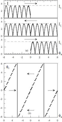
Figure 3: The maximum supercurrent $I_{m}$ and internal flux $\phi_{i}$ dependencies on the applied flux $\phi_{a}$ for a short junction ($L=0.25\,\Lambda$, $\alpha=2\sqrt{3}$ and $\gamma=6$). The arrows indicate the sweeping direction of the applied flux, the points are for the results of the numerical calculations, and the solid lines are for the surface current $I_{\zeta}(\phi_{a})$ given by Eq. (45).

In Fig. 3 (a) we demonstrate the dependence of the maximum supercurrent on the applied flux, $I_{m}(\phi_{a})$, for a short junction, $L=0.25\,\Lambda$. In agreement with the theoretical results obtained in Sec. III.1 (see Eq. (45)) we find that $I_{m}(\phi_{a})\approx I_{\zeta}(\phi_{a})$ except for small deviations at low fields. In Fig. 3 (b) we plot the internal flux $\phi_{i}$ as a function of the applied flux $\phi_{a}$. It is seen from the graphs that $\phi_{i}\approx\phi_{a}$, which is in agreement with the assumptions of the theoretical calculations of Sec. III.1. Small flux “jumps”, $\Delta\phi\ll\phi_{0}$, are seen in Fig. 3 (b) in the vicinity of $\phi_{a}=n\phi_{0}$, where $n$ is an integer. These small flux jumps are generated by the high density screening currents $\sim\langle|j_{c}(x)|\rangle\gg\langle j_{c}(x)\rangle$ flowing at the edges of the junctions. The length of these current-carrying edges is of the order of $l$ and therefore the value of $\Delta\phi$ can be estimated as follows. First, using Maxwell equations we find the field drop $\Delta H$ at the edges to be $\Delta H\approx 4\pi\langle|j_{c}|\rangle l/c$. Next, we estimate $\Delta\phi$ as a product of the field drop $\Delta H$ and the effective area of the junction, $2\lambda L$, i.e., $\Delta\phi\approx 2\lambda L\Delta H$. Finally, we write the parameter $\alpha$ as $\alpha\approx\langle|j_{c}|\rangle\,l/\langle j_{c}\rangle\Lambda$. Combining these three relations we find an estimate for $\Delta\phi$ in the form

$$\Delta\phi\approx{\alpha\over 2\pi}{L\over\Lambda}\phi_{0}.$$ (96)

It is worth noting that $\Delta\phi$ coincides with the coefficient in Eq. (72) for the difference between the internal flux and the applied flux. Using the data $\alpha=2\sqrt{3}$ and $L=\Lambda/4$ we obtain $\Delta\phi=0.14\phi_{0}$ which is in a good agreement with the flux jumps shown in Fig. 3 (b).

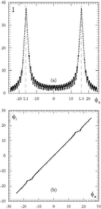
Figure 4: The maximum supercurrent $I_{m}$ and internal flux $\phi_{i}$ dependencies on the applied flux $\phi_{a}$ for a short junction ($L=0.5\,\Lambda$, $\alpha=2\sqrt{3}$ and $\gamma=6$). (a) The function $I_{m}(\phi_{a})$ with two side-picks located at $\phi_{a}=\pm(L/l)\,\phi_{0}$; (b) the dependence $\phi_{i}(\phi_{a})$ exhibiting flux-plateaus at the side-picks.

In this study we assume that the applied field is smaller than the side-picks field $H_{\rm sp}$. The “resonances” at the side-picks are discussed in detail in Ref. Mints and Kogan, 1997 and Buzdin and Koshelev, 2003. We show in Fig. 4 the maximum supercurrent $I_{m}(\phi_{a})$ and internal flux $\phi_{i}(\phi_{a})$ at the side-picks for completeness and to reveal the flux-plateaus appearing in the dependence $\phi_{i}(\phi_{a})$ at $H_{a}=\pm H_{\rm sp}$.

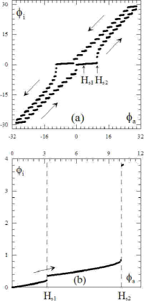
Figure 5: The internal flux $\phi_{i}$ dependence on the applied flux $\phi_{a}$ for a long junction ($L=30\,\Lambda$, $I=0$, $l=0.2\,\Lambda$, $\alpha=0$ and $\gamma=2$). The arrows indicate the direction of sweeping of $\phi_{a}$ for the magnetization cycles starting from $\phi_{a}=0$ and zero trapped flux. (a) The main features of internal flux $\phi_{i}(\phi_{a})$ of long junctions (flux-plateaus, flux jumps and significant hysteresis); (b) the dependence $\phi_{i}(\phi_{a})$ for the applied field $H_{a}$ from the interval $0<H_{a}<H_{\rm s2}$.

In Fig. 5 we show the internal flux $\phi_{i}$ for a long junction, $L=30\Lambda$, as a function of the applied flux $\phi_{a}$. The value of $\phi_{i}$ is less than one flux quanta if the field $H_{a}$ is lower than the second penetration field $H_{\rm s2}$. In this region of fields the slope $d\phi_{i}/d\phi_{a}$ is proportional to $\Lambda/L\ll 1$, i.e., it is almost zero. As a result, for long junctions in low applied fields we observe two relatively long flux-plateaus. These flux-plateaus, flux jumps and significant hysteresis in the magnetization curves $\phi_{i}(\phi_{a})$ are clearly seen in the whole area of $\phi_{a}$. All these features of magnetization curves are in a good agreement with the theoretical results obtained in Sec. III.

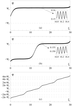
Figure 6: The phase $\varphi$ dependence on the coordinate $\zeta$ for a long junction ($L=30\,\Lambda$, $I=0$, $l=0.2\,\Lambda$, $\alpha=0$, $\gamma=2$). The insets show the oscillatory nature of the function $\varphi(\zeta)$ on the space-scale of order $l$. (a) The applied field is sweeping up, the applied flux $\phi_{a}=0.8\,\phi_{0}$; (b) the phase $\varphi(\zeta)$ is shown after the first flux penetration that occurs at $\phi_{a}=4.6\,\phi_{0}$, the applied field is sweeping up.

In Figs. 6 (a), (b) we show the spatial distributions of the phase $\varphi(\zeta)$ in a long junction, $L=30\,\Lambda$. The graph in Fig. 6 (a) is obtained for a junction in the Meissner state, i.e., for the applied field $H_{a}$ from the interval $0<H_{a}<H_{\rm s1}$. In this case the flux inside the junction is zero. The graph shown in Fig. 6 (b) is calculated for a junction in the one-splinter-vortex intermediate state, i.e., for the applied field from the interval $H_{\rm s1}<H_{a}<H_{\rm s2}$ and the internal flux $\phi_{i}=\phi_{1}$ (see Eq. (58)). These numerical results are in a good agreement with the theoretical calculation of Sec. III.2.

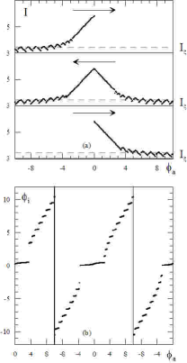
Figure 7: The maximum supercurrent $I_{m}$ and the internal flux $\phi_{i}$ dependencies on the applied flux $\phi_{a}$ for a long junction ($L=20\,\Lambda$, $\alpha=\sqrt{3}$, $\gamma=1.5$). The arrows indicate the direction of sweeping of $\phi_{a}$ and the points are for the results of the numerical calculations.

In Fig. 7 (a) we plot the maximum value of the supercurrent $I_{m}$ as a function of the applied flux $\phi_{a}$ for a long junction, $L=20\,\Lambda$. At low applied flux the maximum current is linearly dependent on $|H_{a}|$ yielding the middle triangle in agreement with Eq. (69). If the applied flux is sweeping up then the maximum current in the mixed state is higher than the maximum current in the Meissner state $H_{a}=H_{s2}-4\pi\alpha I_{c}/c$ and flux penetrates into the junction (flux jump) and the dependence $I_{m}(\phi_{a})$ changes. If the applied field is sufficiently high then the maximum current is approximately equal to $2\alpha I_{c}$ in agreement with Eq. (82). In Fig. 7 (b) we plot the internal flux $\phi_{i}$ as a function of the applied flux $\phi_{a}$. As it is assumed for fields lower than the first penetration field the junction is in the Meissner state. When sweeping the field from low to high fields the flux penetrates into the junction at $H_{a}=H_{s2}-4\pi\alpha I_{c}/c$ yielding a finite flux density. When sweeping the field from high to low values the Josephson vortices leave the junction one by one yielding the additional two steps between the plateau and the mixed state. In the interval of high applied fields the flux jumps are of order of one flux quanta $\phi_{0}$ and in between the flux is almost constant in agreement with Eq. (79).

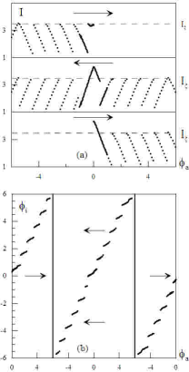
Figure 8: The maximum supercurrent $I_{m}$ and internal flux $\phi_{i}$ dependencies on the applied flux $\phi_{a}$ for a junction with an intermediate length ($L=2\,\Lambda$, $\alpha=2\sqrt{3}$, $\gamma=6$). The points are for the results of numerical simulations. The arrows indicate the direction of sweeping of the applied flux.

In Fig. 8 (a) we plot the maximum current as a function of the applied flux for a junction with an intermediate length $L=2\,\Lambda\sim\Lambda$. In Fig. 8 (b) we plot the flux $\phi_{i}$ as a function of the applied flux. It is seen that the flux $\phi_{i}$ differs from the applied flux $\phi_{a}$ by less then one flux quantum $\phi_{0}$ as for the short junctions. The flux jumps happen at $\phi_{a}=(n+1/2)\phi_{0}$, where $n$ is an integer. The value of $\Delta\phi$ is well approximated by Eq. (96).

V Summary

To summarize, we consider theoretically and numerically the maximum supercurrent across Josephson tunnel junctions with a critical current density, which is rapidly alternating along the junction. These complex Josephson tunnel systems were treated recently in asymmetric grain boundaries in thin films of high-temperature superconductor YBa₂Cu₃O_7-x and in superconductor-ferromagnet-superconductor heterostructures.

Our theoretical study is based on coarse-grained sine-Gordon equation. We derive boundary conditions to this equation and find explicit dependencies of the maximum supercurrent across a junction on the magnetic field in the Meissner and mixed states for short and long junctions. We show that in the case of a Josephson junction with rapidly alternating critical current density there can exist one-splinter-vortex mixed state and two flux-penetration fields. The obtained theoretical results are verified by numerical simulations of exact sine-Gordon equation. We demonstrate that the theoretical and numerical results are in a good agreement.

References

• Bulaevskii et al. (1977) L. N. Bulaevskii, V. V. Kuzii, and A. A. Sobyanin, JETP Letters 25, 290 (1977).
• Buzdin et al. (1982) A. I. Buzdin, L. N. Bulaevskii, and S. V. Panjukov, JETP Lett. 35, 178 (1982).
• Ryazanov et al. (2001) V. V. Ryazanov, V. A. Oboznov, A. Y. Rusanov, A. V. Veretennikov, A. A. Golubov, and J. Aarts, Phys. Rev. Lett. 86, 2427 (2001).
• Kontos et al. (2002) T. Kontos, M. Aprili, J. Lesueur, F. Genet, B. Stephanidis, and R. Boursier, Phys. Rev. Lett. 89, 137007 (2002).
• Blum et al. (2002) Y. Blum, A. Tsukernik, M. Karpovski, and A. Palevski, Phys. Rev. Lett. 89, 187004 (2002).
• Buchal et al. (1995) C. Buchal, C. A. Copetti, F. R$\ddot{u}$ders, B. Oelze, B. Kabius, and J. W. Seo, Physica C 253, 63 (1995).
• Hilgenkamp et al. (1996) H. Hilgenkamp, J. Mannhart, and B. Mayer, Phys. Rev. B 53, 14586 (1996).
• Van Harlingen (1995) D. J. Van Harlingen, Rev. Mod. Phys. 67, 515 (1995).
• Tsuei and Kirtley (2000) C. C. Tsuei and J. R. Kirtley, Rev. Mod. Phys. 72, 969 (2000).
• Hilgenkamp and Mannhart (2002) H. Hilgenkamp and J. Mannhart, Rev. Mod. Phys. 74, 485 (2002).
• Mannhart et al. (1996) J. Mannhart, H. Hilgenkamp, B. Mayer, C. Gerber, J. R. Kirtley, K. A. Moler, and M. Sigrist, Phys. Rev. Lett. 77, 2782 (1996).
• Mints and Kogan (1997) R. G. Mints and V. G. Kogan, Phys. Rev. B 55, R8682 (1997).
• Mints (1998) R. G. Mints, Phys. Rev. B 57, R3221 (1998).
• Mints et al. (2002) R. G. Mints, I. Papiashvili, J. R. Kirtley, H. Hilgenkamp, G. Hammerl, and J. Mannhart, Phys. Rev. Lett. 89, 067004 (2002).
• Buzdin and Koshelev (2003) A. Buzdin and A. E. Koshelev, Phys. Rev. B 67, 220504(R) (2003).
• Landau and Lifshitz (1976) L. D. Landau and E. M. Lifshitz, Mechanics (Pergamon Press, 1976).
• Arnold and Neishtadt (1997) V. V. Arnold, V. I. Kozlov and A. I. Neishtadt, Mathematical aspects of classical and celestial mechanics (Springer, 1997), 2nd ed.
• Golubov et al. (2004) A. A. Golubov, M. Y. Kupriyanov, and E. Il’ichev, Rev. Mod. Phys. 76, 411 (2004).
• Kulik and Janson (1972) I. O. Kulik and I. K. Janson, The Josephson effect in superconductive tunnelling structures (Jerusalem, 1972).
• Barone and Paterno (1982) A. Barone and G. Paterno, Physics and Applications of the Josephson Effect (Wiley, New York, 1982).
• Owen and Scalapino (1967) C. S. Owen and D. J. Scalapino, Phys. Rev. 164, 583 (1967).