STAR FORMATION IN THE EXTREME OUTER GALAXY:
DIGEL CLOUD 2 CLUSTERS

Abstract

As a first step for studying star formation in the extreme outer Galaxy (EOG), we obtained deep near-infrared ($J,H,K$-bands) images of two embedded clusters at the northern and southern CO peaks of Cloud 2, which is one of the most distant star forming regions in the outer Galaxy (galactic radius $R_{g}\sim 19$ kpc). With high spatial resolution (FWHM $\sim 0\farcs 3$–$0\farcs 35$) and deep imaging ($K\sim 21$ mag, 5 $\sigma$) with the IRCS imager at the Subaru telescope, we detected cluster members with a mass detection limit of $<0.1M_{\odot}$, which is well into the substellar regime. These high quality data enables a comparison of EOG to those in the solar neighborhood on the same basis for the first time. Before interpreting the photometric result, we have first constructed the NIR color-color diagram (dwarf star track, classical T Tauri star (CTTS) locus, reddening law) in the Mauna Kea Observatory filter system and also for the low metallicity environment since the metallicity in EOG is much lower than those in the solar neighborhood. The estimated stellar density suggests that an “isolated type” star formation is ongoing in Cloud 2-N, while a “cluster type” star formation is ongoing in Cloud 2-S. Despite the difference of the star formation mode, other characteristics of the two clusters are found to be almost identical: (1) $K$-band luminosity function (KLF) of the two clusters are quite similar, as is the estimated IMF and ages ($\sim 0.5$–1 Myr) from the KLF fitting, (2) the estimated star formation efficiencies (SFEs) for both clusters are typical compared to those of embedded clusters in the solar neighborhood ($\sim 10$ %). The similarity of two independent clusters with a large separation ($\sim 25$ pc) strongly suggest that their star formation activities were triggered by the same mechanism, probably the supernova remnant (GSH 138-01-94) as suggested in Kobayashi et al. and Yasui et al.

1. Introduction

The extreme outer Galaxy (hereafter “EOG”), defined here as the region at Galactic radius ($R_{g}$) greater than 18 kpc, could be regarded as the outermost region of the Galaxy because the distribution limits of Population I and II stars are known to be 18–19 kpc and 14 kpc, respectively (Digel et al., 1994). The EOG is known to have very low gas density (Brand & Wouterloot, 1995; Nakanishi & Sofue, 2003) and low metallicity (Smartt & Rolleston, 1997). Such an extreme environment could serve as a “laboratory” for studying the star formation process in a totally different environment from that in the solar neighborhood. The star-forming process in such environments has not been studied extensively as for the nearby star-forming regions because of the large distance. The EOG does not seem to have long and complex star formation history because there is little or no perturbation from the spiral arms, which is the major and powerful trigger for continuously converting a large amount of molecular gas into stars. Therefore, in the EOG there is a good chance to observe the detail of the each star formation process, such as the triggering process of cluster formation, without being disturbed by the entangled star formation history in space and time.

There are some synthetic studies of molecular clouds in EOG and far outer Galaxy (hereafter “FOG”), whose $R_{g}$ is not more than 18 kpc but no less than 15 kpc. The pioneering survey of molecular clouds and star formation beyond the solar circle was undertaken by Wouterloot & Brand (1989), who identified the ¹²CO molecular emission associated with color-selected IRAS point sources and used kinematic distances to place the sources within the Galaxy. Many of the IRAS sources were found to lie in the far outer Galaxy. Follow-up studies of the gas properties of many of these far outer Galaxy molecular clouds were presented in Brand & Wouterloot (1994, 1995) separately. In an independent search, Digel et al. (1994) found eleven molecular clouds in the EOG, based on CO observations of distant H I peaks in the Maryland-Green Bank survey (Westerhout & Wendlandt, 1982). Following those pioneering works, Heyer et al. (1998) conducted a comprehensive CO survey of molecular clouds in the FOG with Five College Radio Astronomy Observatory (FCRAO) CO survey. With H$\alpha$ and radio continuum study, Fich & Blitz (1984), Brand & Blitz (1993), and Rudolph et al. (1996) identified a number of H II regions associated with the FOG clouds, indicating the presence of recent massive star formation.

For the study of star formation, it is ultimately necessary to observe YSOs (young stellar objects) at near infrared (NIR) wavelengths. Kobayashi & Tokunaga (2000) found YSOs associated with a molecular cloud in EOG for the first time with a wide-field NIR survey. This cloud is denoted as Cloud 2 in the list of Digel et al. (1994) and is one of the most distant molecular clouds in the outer Galaxy region. It is located at a very large Galactic radius ($R_{g}=18$–28 kpc) in the second quadrant of the Galaxy ($l\sim 137.75^{\circ}$, $b\sim-1.0$). It is by far the largest molecular cloud among those found in EOG with a mass comparable to that giant molecular clouds ($M\sim 2\times 10^{4}$ $M_{\odot}$; Digel et al. 1994). The Galactic radius of Cloud 2 has been estimated by various methods at $R_{g}=28$ kpc (heliocentric distance: $D=21$ kpc) from the kinematic distance of the CO cloud (Digel et al., 1994); $R_{g}=23.6$ kpc ($D=16.6$ kpc) from the latest H I observation (Stil & Irwin, 2001); and $R_{g}=15$–19 kpc ($D=8.2$–12 kpc) from the detailed optical study of a B-type star, MR1 (Muzzio & Rydgren, 1974; Smartt et al., 1996), which is associated with Cloud 2 (de Geus et al., 1993). Throughout this paper we adopt $R_{g}=19$ kpc ($D=12$ kpc) because it is about the mean value of all the estimated distances and because spectroscopic distance of stars should be more accurate than kinematic distance. Metallicity at the Galactic radius of Cloud 2 is estimated to be $\sim-1$ dex from the standard metallicity curve by Smartt & Rolleston (1997). In fact, the metallicity of the B-type star, MR1, is measured at $-0.5$ to $-0.8$ dex by optical high-resolution spectroscopy (Smartt et al., 1996; Rolleston et al., 2000) and that of the Cloud 2 itself is measured at $-0.7$ dex from the radio molecular emission lines (Lubowich et al., 2004; Ruffle07). These metallicity values are comparable to that of LMC ($\sim-0.5$ dex) and SMC ($\sim-0.9$ dex; Arnault et al., 1988). Using deeper near-infrared imaging with QUIRC at the University of Hawaii (UH) 2.2m telescope, Kobayashi et al. (2007) also found two embedded clusters at the northern and southern CO peaks of Cloud 2. They suggested that the overall star formation activity in Cloud 2 was triggered by the supernova remnant (SNR) H I shell, GSH 138-01-94, and that supernova triggered star formation could be one of the major star formation modes in EOG.

Recently Brand & Wouterloot (2007) reported comprehensive study of a star forming region, WB89-789, whose distance is estimated at $D=11.9$ kpc, $R_{g}\sim 20.2$ kpc. This region was found in Wouterloot & Brand (1989) described above. They obtained NIR imaging with limiting magnitude of $m_{K}=16.5$ and 17.5 mag for 10 $\sigma$ and 5 $\sigma$, respectively, which correspond to a 2–3 $M_{\odot}$ dwarf main sequence star with 10 mag of visual extinction. They also used molecular line and dust continuum observations for properties of the molecular cloud and showing the existence of an outflow. They also obtained optical spectroscopy of a star for confirmation of the distance to the region. Santos et al. (2000) discovered two distant embedded young clusters in the FOG ($R_{g}=16.5$ kpc; $D=10.2$ kpc) with near-infrared imaging of CO clouds associated with IRAS sources. Their detection limit ($m_{K}=16.4$ mag) corresponds to a 1 Myr old star of $\sim$1–2 $M_{\odot}$ seen through 10 mag of visual extinction. Snell et al. (2002) have conducted a comprehensive NIR survey of embedded clusters in the FOG ($R_{g}=13.5$–17.3 kpc) based on the FCRAO CO survey (Heyer et al., 1998). They found 11 embedded clusters with the detection limit of $m_{K^{\prime}}$=17.5 mag. For their most distant cluster, this magnitude corresponds to a 1 Myr old, 0.6 $M_{\odot}$ star with no extinction, or a 1 Myr old, 1.3 $M_{\odot}$ star seen through 10 mag of visual extinction. These independent near-infrared searches so far found cluster members with the mass detection limit of $\sim 1$ $M_{\odot}$.

As a next step to study the details of the star formation activity in the EOG, we obtained deep and high spatial resolution NIR images of the two most distant embedded clusters in Digel Cloud 2 with Subaru 8.2-m telescope. Because of the achieved sensitivity to detect substellar mass members, we could compare embedded clusters in EOG to those in the solar neighborhood for the first time. In Yasui et al. (2006, hereafter Paper I), we presented the data for the Cloud 2-N cluster and (i) estimated the age of the cluster at less than 1 Myr by comparing the observed KLF to model KLFs based on typical IMFs, and (ii) suggested that the formation of the cluster was triggered by the SNR shell based on the age and the geometry of the cluster. In this paper, we present data of the Cloud 2-S cluster and also re-analyze the data of Cloud 2-N cluster to investigate the fainter stellar population. For interpreting the photometric result, we have constructed for the first time the NIR color-color diagram (dwarf track, CTTS locus, and reddening vector) in the Mauna Kea Observatory (MKO) near-infrared filter system (Simons & Tokunaga, 2002; Tokunaga et al., 2002). To accommodate to the low-metallicity in EOG, we also considered the mass-luminosity relation and the color-color diagram for low metallicity stars. The established methods here would be useful for future study of star formation in EOG and FOG, and ultimately nearby dwarf galaxies. We then discuss the KLF and star formation efficiency in the EOG based on the results of these two clusters.

2. Observations and Data Reduction

2.1. Subaru IRCS imaging

We obtained $J$ (1.25 $\mu$m), $H$ (1.65 $\mu$m), $K$ (2.2 $\mu$m)-band deep images of the Cloud 2-N and -S clusters with the Subaru Infrared Camera and Spectrograph (IRCS; Tokunaga et al. 1998; Kobayashi et al. 2000; Terada et al. 2004) with a pixel scale of $0\farcs 058$ pixel^-1. IRCS employs the Mauna Kea Observatory (MKO) near-infrared photometric filters (Simons & Tokunaga, 2002; Tokunaga et al., 2002). The entire infrared cluster was sufficiently covered with the $\sim 1^{\prime}$ field of view. For the Cloud 2-N cluster, the observation was conducted on 2000 December 1 UT with the total integration time of 600, 450, 900 s for $J$, $H$, and $K$ bands, respectively. For the Cloud 2-S cluster, the observation was conducted on 2000 October 25 UT with the total integration time of 600, 600, 420 s for $J$, $H$, and $K$ bands, respectively. The observing condition was photometric and the seeing was excellent ($\sim 0\farcs 3$–$0\farcs 35$) throughout the observing period on both nights.

2.2. Data Reduction

All the data for each band were reduced with IRAF with standard procedures: dark subtraction, flat fielding, bad-pixel correction, median-sky subtraction, image shifts with dithering offsets, and combining. In our previous paper (Paper I), we used the DAOFIND algorithm in IRAF DAOPHOT package with the detection threshold of 10 $\sigma$ for the source detection in the Cloud 2-N cluster. In the present study, we performed source detection for the Cloud 2-N cluster again and the Cloud 2-S cluster using SExtractor (Bertin et al. 1996) with the detection threshold of 5 $\sigma$ above the local background. Photometry was performed using IRAF APPHOT package with aperture diameters of $0\farcs 58$ (10 pixel) and $0\farcs 46$ (8 pixel), for Cloud 2-N and -S, respectively. The aperture sizes were chosen to achieve the highest S/N. For four pairs of binary stars in the Cloud 2-N cluster, $0\farcs 35$ (6 pix) diameter aperture was applied with an aperture correction because the separation is less than $0\farcs 5$. For photometric calibration we used four and seven bright and isolated stars for the Cloud 2-N and -S cluster, respectively, in the images for which photometry was accurately done later with newly obtained $JHK$ images of the fields with Subaru’s new wide-field near-infrared camera MOIRCS (Ichikawa et al. 2006). The flux uncertainties are estimated as the same way as in Paper I. The resultant limiting magnitudes (5 $\sigma$) for the Cloud 2-N cluster are $J=22.0$, $H=21.0$, and $K=20.9$, while those for the Cloud 2-S cluster are $J=21.8$, $H=21.0$, and $K=20.4$. The pseudocolor images of the observed field and the spatial distributions of detected stars are shown in Figs. 1 and 2 for the Cloud 2-N cluster and -S cluster, respectively.

3. Color-Color Diagram in MKO Photometric System

For identifying of young cluster members, $JHK$ color-color diagram with dwarf and giant star tracks in Johnson-Glass system (Bessel & Brett, 1988, hereafter “B&B”), CTTS locus in CIT system (Meyer et al., 1997), and reddening vector in Arizona system (Rieke & Lebofsky, 1985) have been widely used (e.g., Lada et al., 2000). Because the Mauna Kea Observatory (MKO) filter system (Simons & Tokunaga, 2002; Tokunaga et al., 2002), which we used for the present study, is relatively new, the color-color diagram in this system have not yet been clearly established. Although we used the color-color diagram with the dwarf track etc. in other systems in our previous paper (Paper I), we constructed a color-color diagram solely in the MKO system for more rigorous treatment of the data.

Firstly, we plotted colors of dwarf stars observed with MKO filters (Hewett et al. 2006, open circle, B9V–M6V; Leggett et al. 2002, plus, M4V–M6V; Leggett et al. 2006, cross, M4–M6) to construct a dwarf track in the MKO system (solid line). Although this MKO track appears to be almost identical to the B&B track for stars earlier than K type stars, the MKO track has a smaller $J-H$ color than the B&B track for M type stars. Because the MKO $J$ filter has a narrower band width compared to the other filter systems (see Fig. 5 in Stephens & Leggett, 2004), the MKO $J$ magnitude is less affected by the strong H₂O vapor absorption bands of M type stars. This should result in a brighter $J$ magnitude, thus the smaller $J-H$ color in the MKO system. We interpret this as the reason for the shift of the track position for M type stars and also the reason why the shift becomes larger with later spectral type.

Secondly, in order to construct the CTTS locus in the MKO system, we checked the 2MASS $J,H,K$-band magnitudes of classical T Tauri stars in Strom et al. (1989), which were used to derive the original CTTS locus in the CIT system Meyer et al. (1997). After dereddening the 2MASS colors of these stars following the method of Meyer et al. (1997) with the reddening law in Cambrésy et al. (2002), we converted the 2MASS colors to the MKO colors using the conversion in Leggett et al. (2006). We derived the CTTS locus in MKO system by least-square fitting of the MKO colors: the resultant locus is $(J-H)_{\rm MKO}=(0.32\pm 0.07)(H-K)_{\rm MKO}+(0.54\pm 0.04)$. Compared to the original CTTS locus, $(J-H)_{\rm CIT}=(0.58\pm 0.11)\times(H-K)_{\rm CIT}+(0.52\pm 0.06)$, the MKO locus has smaller $J-H$ with increasing $H-K$. This tendency is consistent with that for the dwarf track as discussed above.

Lastly, we considered the reddening vector, which is the the slope $(J-H)/(H-K)$ and the length of the $A_{V}=5$ mag vector. Using the near-infrared camera SIRIUS equipped with the MKO filters, Nishiyama et al. (2006) estimated that $(J-H)/(H-K_{S})=1.72$ from the data toward the Galactic Center. This value is almost identical to the conventional slope ($J-H/H-K=1.70$) in Arizona system (Rieke & Lebofsky, 1985). Although IRSF uses a $K_{S}$ band filter instead of a $K$ band filter, the difference of the filter profile is so small (see Fig. 1 in Tokunaga et al., 2002) that the magnitude differences are negligible. Therefore, we could conclude that the reddening vector is almost identical for both Arizona and MKO systems. In the following section, we use the MKO color-color diagram for all the analysis.

4. Color-Color Diagram for Low Metallicity Environment

Because the metallicity in EOG is significantly lower than in the solar neighborhood, we should consider the effect of low metallicity on the color-color diagram. Following the PMS models by D’Antona & Mazzitelli (1997, 1998), we suggested that NIR absolute magnitudes of PMS stars with $-0.3$ dex (1/2 solar metallicity) is not significantly different from those with the solar metallicity (Paper I). Therefore colors also should not significantly change down to a metallicity of $-0.3$ dex. In this section we discuss the effect of low metallicity extended to $-1$ dex on the $J-H$ and $H-K$ colors considering both observations and models in the literature.

Leggett (1992) presented NIR photometry of low-mass stars in young disk ([M/H] $\sim 0.0$), young-old disk, old disk ([M/H] $\sim-0.5$), old disk-halo ([M/H] $\sim-1.0$), and halo ([M/H] $<-1.0$), showing that $J-H$ colors of dwarfs between K7 (0.5 $M_{\odot}$) and M5 ($\sim 0.1$ $M_{\odot}$) types decrease by $\sim 0.1$ mag with decreasing metallicity (Fig. 4). Similar tendency is seen in the model by Girardi et al. (2002), who listed the NIR magnitudes of stars with mass of 0.15–1 $M_{\odot}$ for various metallicities ($Z=0.001,0.004,0.008,$ and 0.019). Although the color values are slightly different for the observation and the Girardi model, both show the quite similar color variation $\Delta(J-H)=-0.1$ for $\Delta$ [M/H] $\sim-1$, which strengthens the validity of the metallicity dependence. However, for the metallicity of Cloud 2 ([M/H] $\sim-0.5$), the dwarf track is still almost identical to the standard B & B dwarf track within the uncertainty (Fig. 4). As for the stars with mass of $\gtrsim 1$ $M_{\odot}$, Girardi et al. (2002) suggested that the colors weakly depend on metallicity.

Nakajima et al. (2005), who observed the LMC ($-0.5$ dex) in the MKO system, suggested that the slope of $(J-H)/(H-K)$ for LMC appears to be consistent with that for solar metallicity (Nishiyama et al., 2006), suggesting that the reddening vector for the LMC metallicity is not significantly different from that for the solar metallicity.

We conclude that dwarf track and reddening vector in $JHK$ color-color diagrams do not strongly depend on the metallicity down to that of the stars in Cloud 2 ($\sim-0.7$ dex). Therefore, we do not include the effects of low metallicity in the following analysis using color-color diagram, such as the identification of cluster members ($\S$ 5.1), the estimation of extinction and color excess ($\S$ 5.2).

5. RESULTS

5.1. Identification of Cluster Members

We conducted identification of the cluster members using pseudocolor pictures of the observed fields (Fig. 1, 2) and $(J-H)$ vs. $(H-K)$ color-color diagrams of all the detected sources (Fig. 5). We identified cluster members which have color of $(H-K)\gtrsim 0.5$ and are within the cluster regions as identified in Kobayashi et al. (2007). Because there are no foreground molecular clouds in front of Cloud 2 (Kobayashi & Tokunaga 2000), the red colors of the cluster members should originate from the extinction by Cloud 2 itself as well as by circumstellar material (see $\S$ 5.2 for more discussion). Contamination from the background sources should be very small in view of the large $R_{g}$ of Cloud 2.

We found 72 cluster members in the Cloud 2-N cluster and 66 cluster members in the Cloud 2-S cluster. We also identified 10 YSOs in the Cloud 2-S sub-cluster (Kobayashi et al. 2007), which is $\sim 40^{\prime\prime}$ northern-east from the Cloud 2-S cluster. Fig. 1 and Fig. 2 show the spatial distributions of these cluster members and field stars in the Cloud 2-N and -S fields, respectively. Because of the re-analysis with the fainter detection limit, the number of identified Cloud 2-N cluster members has increased from 52 in Paper I to 72.

5.2. Extinction and Disk Color Excess of Cluster Members

The extinction and disk color excess for each star were estimated using the color-color diagram. For reliable estimation of the parameters, only stars in the positions reddened from the CTTS locus and the dwarf locus are used (42 cluster members and 36 field stars for the Cloud 2-N cluster, 45 cluster members and 45 field stars for the Cloud 2-S cluster). For convenience the dwarf locus was approximated by the extension of the CTTS locus drawn out to $H-K\sim 0.1$ mag. In the color-color diagram the extinction $A_{V}$ of each star was estimated from the distance along the reddening vector between its location and the stellar loci. The resultant $A_{V}$ distributions of Cloud 2-N and Cloud 2-S cluster members (Fig. 6) have peak at 7.2 and 6.1 mag, respectively ($A_{K}=0.81$ and 0.68 mag) and those for field stars in the both Cloud 2 fields have a peak at 2.2 mag ($A_{K}=0.25$ mag). The distributions of the both clusters’ members show that the both clusters are reddened uniformly by about $A_{V}\sim 4$–5 mag inside Cloud 2. This verifies the selection method of cloud members as described in $\S$ 5.1. These values of $A_{V}$ are also consistent with the estimated from sub radio and continuum observation (Ruffle et al. 2007).

We also constructed the distributions of the unreddened color $(H-K)_{0}$ of the cluster members and the field stars (Fig. 7). For both clusters, the distributions of the cloud members and field stars show the clear peak offset of about 0.1 mag. The difference of the average $(H-K)_{0}$ between the cluster members and the field stars (Cloud 2-N cluster: 0.26 mag, Cloud 2-S cluster: 0.37 mag) can be attributed to thermal emission of circumstellar disks of the cluster members. Assuming that disk emission appears in the $K$ band but not in the $H$ band, the disk color excess of the Cloud 2-N and -S cluster members in the $K$ band, $\Delta K_{\rm disk}$, is equal to 0.26 and 0.37 mag, respectively.

6. DISCUSSION

6.1. Stellar Density Variation

Lada & Lada (2003) compiled a catalog of embedded clusters that are located in $D\lesssim 2$ kpc (distance modulus DM $<11.5$ mag) and detected cloud members with the apparent limiting magnitudes of $m_{K}\sim 16.0$ mag. Carpenter (2000) analyzed 2MASS data of the Perseus, Orion A, Orion B, and Monoceros R2 clusters at $D\simeq 500$ pc (DM $\simeq 8.5$ mag) and detected members with apparent limiting magnitudes of $m_{K_{S}}=14.3$ mag. Both catalogs thus consist of clusters that are detected with absolute limiting magnitude of $M_{K}\sim 5$–6 mag in the solar neighborhood. In the present study, since the Cloud 2 clusters at $D\sim 12$ kpc (DM $=15.4$ mag) are detected with apparent magnitudes of $m_{K}\sim 20.5$ mag, the absolute limiting magnitudes is $M_{K}\sim 5$ mag. Therefore, we can compare the stellar density of embedded clusters in EOG to those of embedded clusters in the solar neighborhood on the same basis for the first time.

Adams et al. (2006) found a correlation between the number of stars in a cluster and the radius of the cluster, using the tabulated cluster properties in Lada & Lada (2003) and Carpenter (2000) (Fig. 8). Allen et al. (2007) suggested that the average stellar density of clusters have a few to a thousand members varies by a factor of only a few. Stellar densities of the Cloud 2-N and -S clusters were estimated at 13 pc^-2 and 50 pc^-2 from the spatial distribution of the identified cluster members in the $2\times 2$ pc² area and a circle of 0.6 pc radius, respectively. For the Cloud 2-N cluster, the above density is a little larger than our old estimate in Paper I ($\sim 10$ pc^-2) because we included the newly identified fainter stars. In Fig. 8, the Cloud 2-N cluster appears to be a kind of “loose cluster”, while the Cloud 2-S cluster appears to be a kind of “dense cluster”. For the typical stellar density of the clusters ($\sim 50$ pc^-2, see Figure 8), the average projected distance between two adjacent stars is $\sim 0.14$ pc, which corresponds to $\sim 2^{\prime\prime}$ at $D=12$ kpc. For even densest clusters with $\sim 1000$ pc^-2, the average projected distance is $\sim 0.03$ pc, or $0\farcs 5$ at $D=12$ pc. These separations are sufficiently resolved for this observation. Even if all the stars are unresolved binaries, the “loose” and “dense” characteristics of the Cloud 2 clusters do not change (see gray circles in Figure 8). The difference of the stellar densities is very interesting, because the two clusters show very similar characteristics for other points as shown in the following subsections. Kobayashi et al. (2007) attributed the difference of the star formation mode to the ambient pressure difference of the two clusters.

6.2. IMF and Age of the Clusters

$K$-band luminosity functions (KLFs), which are the number of stars as a function of $K$-band magnitude, of different ages are known to have different peak magnitudes and slopes (Muench et al. 2000). IMFs and ages of young clusters can be estimated by comparison of the observed KLF with model KLFs, which are constructed from IMFs and $M$-$L$ relations. In this section, we use the model KLF from Paper I (see $\S$ 4). Although the popular PMS evolution models such as D’Antona & Mazzitelli (1997, 1998), Siess et al. (2000), and Baraffe et al. (1997), do not have models for metallicity less than 1/2 solar ($-0.3$ dex). We assumed that the $M$-$L$ relation for solar metallicity can be applied to model KLFs for low metallicity because the difference of $M$-$L$ relations for the solar metallicity and those for 1/2 solar metallicity is very little (see more detail in Paper I).

Following the method in Paper I, we constructed KLFs of the Cloud 2 cluster members (Fig. 9). We estimated the detection completeness in each magnitude bin by putting artificial stars on random positions in the field and checking whether they are detected in the same way as for the real objects. Five stars are placed at a time in each magnitude bin and the check was conducted 200 times, resulting in about 1000 artificial stars per magnitude bin. The result is also shown in Fig. 9 (bottom), and the completeness-corrected KLFs are shown in Fig. 9 (top) with thick lines. Both KLFs appear to be very similar in the slope at brighter magnitude side and the peak position ($\sim 19$ mag).

The comparison of the completeness corrected KLFs with the model KLFs are shown in Fig. 10. Because the slope of model KLF does not significantly depend on small difference of underlying IMFs (see Fig. 6, 7 in Paper I, ), we used the Trapezium IMF(Muench et al., 2002), which is thought to be the most reliable IMF for young clusters (e.g., Lada & Lada 2003). A quick visual check of Fig. 10 suggests that the ages of the Cloud 2-N and -S clusters are similar and it is $\sim 0.5$–1 Myr. It is difficult to estimate the age of the cluster with an accuracy of 0.1 Myr because isochrone models for ages of less than 1 Myr is thought to be uncertain (e.g., Baraffe et al., 2002). However, we can at least conclude that the ages of the two clusters are no more than 1 Myr (see $\S$ 5.1 in Paper I, ). For the Cloud 2-N cluster, twenty cluster members are detected in the $K\sim 20$ magnitude bin and more in the fainter magnitude bins, while only four members were detected in the $K\sim 20$ magnitude in (the faintest bin) Paper I. However, this change in the fainter bins ($K\gtrsim 20$) did not affect the age estimation, because the brighter bins ($K<19$) are more sensitive for the KLF fitting. The relatively good fit of the model KLF to the observed KLF suggests that the IMF at $M>0.1$ $M_{\odot}$ in Cloud 2 is not significantly different from the “universal” IMF for Trapezium (see also discussion in Paper I).

The similarities of the KLFs and the estimated ages for the two independent clusters with a large separation ($\sim 25$ pc) strongly suggest that their star formation activities were triggered by the same mechanism. The ages of the clusters were estimated at $\sim 0.5$–1 Myr, which is much less than that of the SNR H I shell (GSH 138-01-94; Stil & Irwin 2001), 4.3 Myr. An independent age estimate of the Cloud 2-N cluster ($\sim 0.5$–1 Myr) by Kobayashi et al. (2007) is in quite good agreement with our estimate. These age estimates strongly support the idea that the star formation activity in Cloud 2 was triggered by the SNR H I shell, as discussed in Paper I and Kobayashi et al. (2007).

6.3. Star Formation Efficiency (SFE)

The star formation efficiency (SFE), which is generally defined as [SFE = $M_{\rm stars}/(M_{\rm gas}+M_{\rm stars})$] where $M_{\rm gas}$ is cluster-forming core mass and $M_{\rm stars}$ is the total stellar mass, is one of the most fundamental parameters of the star and cluster-formation processes (Lada & Lada, 2003). The estimated SFEs of the Cloud 2 clusters could be “pure” SFE of one-time cluster formation event because there has been no complex star formation history in the EOG. As discussed in $\S$ 6.1, the detection of the embedded cluster members in the EOG with the high-sensitivity ($m_{K}\simeq 21.0$ mag) enables a fair comparison of SFE in the EOG with that in the solar neighborhood. However, because SFEs have been estimated (e.g., Lada, 1992; Lada et al., 1997; Hartmann, 2002) in various ways, ex. $M_{\rm gas}$ is estimated using different kinds of molecular emission lines (¹²CO, ¹³CO, and C¹⁸O), $M_{\rm stars}$ is estimated with a very simple assumption that all stars have a mass of 1 $M_{\odot}$, 0.5 $M_{\odot}$, etc., here we attempted to estimate SFEs of various star forming regions in a uniform fashion as described in the following paragraphs.

For the estimates of $M_{\rm gas}$ we use ¹³CO because of the relatively high sensitivity even for distant molecular clouds and also the wide availability of the archival data. Because $M_{\rm gas}$ from ¹³CO correlates well with those from C¹⁸O (C¹⁸O–¹³CO mass correlation; Ridge et al., 2003, Fig. 18 (a)), it is possible to use C¹⁸O data when ¹³CO data is unavailable. For the accurate estimation of $M_{\rm stars}$, it is necessary to take the mass of the low mass stars into account. We use a summary of $M_{\rm stars}$ for star forming molecular clouds in the solar neighborhood ($D\lesssim 2$ kpc; Lada & Lada, 2003, Tab. 1). They derived $M_{\rm stars}$ for each cluster by predicting infrared source counts, down to 0.017 $M_{\odot}$ stars, as a function of differing limiting magnitudes using the KLF models of Muench et al. (2002). As an example, we estimated the SFE of the well-known embedded cluster, NGC 1333, which is in the star forming region in Taurus, at 5.2 % using $M_{\rm gas}=1450$ $M_{\odot}$ from ¹³CO (Warin et al. 1996) and $M_{\rm stars}=79$ $M_{\odot}$. We also estimated the SFE of the NGC 2024 at 17 % using $M_{\rm gas}=896$ $M_{\odot}$ from C¹⁸O (Lada et al. 1991a,b) and the C¹⁸O–¹³CO mass correlation (Ridge et al. 2003), and $M_{\rm stars}=182$ $M_{\odot}$. Of 76 embedded clusters in the solar neighborhood (Lada & Lada, 2003), the SFEs for 30 embedded clusters, whose $M_{\rm gas}$ could be found in the literatures, are estimated in the same way, resulting in the SFEs widely ranging from 2.3 to 57 % with an median of 15 %. Median size and mass of the cluster-forming cores are $0.6$ pc (0.32–1.0 pc in FWHM) and $M_{\rm gas}=480$ $M_{\odot}$ (27–4000 $M_{\odot}$), respectively, while median size and mass of embedded clusters are 0.62 pc (0.3–1.9 pc) and $M_{\rm stars}=66$ $M_{\odot}$ (25–340 $M_{\odot}$), respectively.

The spatial distribution of the Cloud 2 cluster members (red crosses) and the molecular cloud cores (blue contour for ¹³CO and gray scale for ¹²CO) are shown in Fig. 11. $M_{\rm stars}$ of the Cloud 2-N and -S clusters are estimated at 48 and 46 $M_{\odot}$, respectively, by directly counting the stellar mass of all cluster members larger than mass detection limit ($<0.1M_{\odot}$) using the model KLF at the age of 0.5 Myr constructed in $\S$ 6.2. Even if we estimate $M_{\rm stars}$ with the stars down to 0.017 $M_{\odot}$ as the same way in Lada & Lada (2003), the $M_{\rm stars}$ increases only $\sim 5$ % . Both sizes of the clusters are typical, whose radii are $\sim 1$ pc for Cloud 2-N and $\sim 0.6$ pc for Cloud 2-S. For $M_{\rm gas}$, because of the large distance to Cloud 2 and the relatively low spatial resolution of radio observations compared to NIR observations, the region of associated core must be carefully assessed. In Fig. 11 the Cloud 2-N core has two sub-peaks which have similar flux, while the Cloud 2-S core appears to be single. Because the Cloud 2-N cluster is associated with the northern sub-peak, we have estimated the $M_{\rm gas}$ for the Cloud 2-N cluster using only the northern part of the cloud. The resultant $M_{\rm gas}$ for the Cloud 2-N and Cloud 2-S clusters are 360 $M_{\odot}$ and 310 $M_{\odot}$ with the radii of 2.7 and 1.7 pc in FWHM, respectively (Saito et al. 2007). As a result, the SFEs of Cloud 2-N, -S clusters are estimated at 12 and 13 %, respectively. These SFEs are comparable to embedded clusters in the solar neighborhood. For FOG, there have been several studies on SFE of star forming molecular clouds. Snell et al. (2002) found that the ratio of far-infrared luminosity to molecular cloud mass in FOG is comparable to that of molecular clouds in the solar neighborhood, suggesting SFE in FOG is similar to that in the solar neighborhood. Our estimates of SFEs in EOG are consistent with these results for FOG. It is also interesting to note that the SFEs for the two independent clusters are similar despite the large difference in the stellar densities (see $\S$ 6.1).

Note that the estimated SFEs still have some systematic uncertainties that should be carefully considered. Firstly, it is possible that some stars were not counted because of confusion with other stars. For example we might miss more close binaries at this large distance. However, even if all stars are binary with the same mass, the SFEs of the Cloud 2-N and -S clusters are 24 % and 26 % respectively. This is not unusual. Secondly, it is possible that we are not still resolving the cloud cores because of the large distance to Cloud 2, thus overestimating the cloud mass by including the mass of unrelated cores. Actually, the radii of Cloud 2 cores ($>2$ pc) are about twice the maximum radius of nearby cores ($<1$ pc), there is a possibility that the Cloud 2 cores are not resolved by a factor of two. In this case, SFEs are underestimated. Lastly, $M_{\rm gas}$ may be underestimated given low metallicity of Cloud 2 because we assume the normal fractional abundance of $X(^{13}$CO) at $2\times 10^{-6}$ in deriving $M_{\rm gas}$. Since the metallicity is lower by a factor of 5 than that in the solar neighborhood, the $X(^{13}$CO) is likely 5 times larger than the assumed value. As a result, $M_{\rm gas}$ may become larger accordingly. In this case, SFEs are overestimated. Of these uncertainties the estimate of $M_{\rm gas}$ is most critical. For more accurate estimate of SFEs, radio observation with higher spatial resolution (e.g., with interferometry) is necessary and a more accurate CO-H₂ conversion factor $X(^{13}$CO) as a function of metallicity is needed.

7. CONCLUSION

We have conducted a pilot study of star formation in EOG using the two embedded clusters in Cloud 2. Our conclusions can be summarized as follows:

1. We have obtained deep near-infrared images of two embedded clusters in EOG, the Cloud 2 clusters, with Subaru 8.2 m telescope and the IRCS infrared imager. This is the first deep infrared imaging of star forming regions in EOG, with the mass detection limit close to the substellar regime ($<0.1M_{\odot}$).

2. Due to the faint detection-limit, we investigated the IMF and age of the clusters in EOG by identifying the peak magnitude of the KLF. The underlying IMF of the cluster down to the detection limit is not significantly different from the typical IMFs in the field and in the nearby star clusters. For investigating the behavior of IMF (KLF) in the substellar regime, even deeper imaging is required and we might find a different IMF than the solar neighborhood. We have estimated the age of the clusters to be $\sim 0.5$–1 Myr. Additionally, SFEs of the Cloud 2 clusters were comparable ($\sim 10$ %) within the uncertainties to nearby embedded clusters. Despite these identical characteristics of the Cloud 2 clusters, the estimated stellar density suggests that different types of star formation are ongoing: an “isolated type” star formation is ongoing in Cloud 2-N, while a “cluster type” star formation is ongoing in Cloud 2-S.

3. We summarized the existing models of near-infrared characteristics of low metallicity stars to derive the mass-luminosity relation and color-color diagram for low metallicity stars. We concluded that dwarf track and reddening vector in $JHK$ color-color diagrams do not strongly depend on the metallicity down to that of the stars in Cloud 2 ($\sim-0.7$ dex). Therefore, we did not include the effects of low metallicity in the following analysis using color-color diagram, such as the identification of cluster members, the estimation of extinction and color excess. However, the effect could be significant for even lower metallicity and more theoretical studies and compilations of the near-infrared data for low-metallicity normal stars are needed.

4. For interpreting the photometric result, we have constructed the NIR color-color diagram (dwarf track, CTTS locus, reddening vector) in the MKO filter system, for which colors for main sequence stars have not been well established before. We find that it is important to carefully compare colors in different photometric systems.

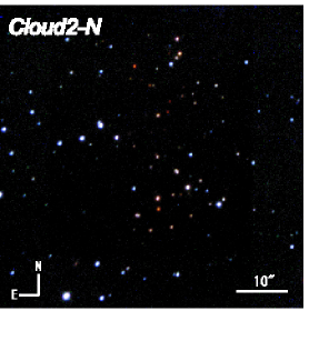
Figure 1.— Left: $JHK$ pseudocolor image of the Cloud 2-N cluster. North is up and east is left. The field of view is about $1^{\prime}\times 1^{\prime}$. The coordinate of the field center is ($\alpha_{\rm 2000},\delta_{\rm 2000}$) = ($02^{h}48^{m}42.5^{s},+58^{\circ}28^{\prime}56\farcs 0$) with an uncertainty of less than 0.5 arcseconds. Right: Spatial distribution of Cloud 2-N cluster members. Filled circles and open circles represent cluster members and field stars, respectively.

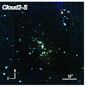
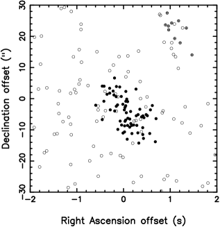
Figure 2.— Left: $JHK$ pseudocolor image of the Cloud 2-S cluster. North is to up and east is left. The field of view is about $1^{\prime}\times 1^{\prime}$. The coordinate of the field center is ($\alpha_{2000},\delta_{\rm 2000}$) = ($02^{h}48^{m}28.7^{s},+58^{\circ}23^{\prime}34\farcs 6$) with an uncertainty of less than 0.5 arcseconds. Right: Spatial distribution of the members of the Cloud 2-S cluster, the Cloud 2-S sub-cluster and field stars are shown with filled circles, circles with cross, and open circles, respectively. The Cloud 2-S sub-cluster was designated at IRS3 in Kobayashi & Tokunaga (2000) as discussed in $\S$ 5.1.

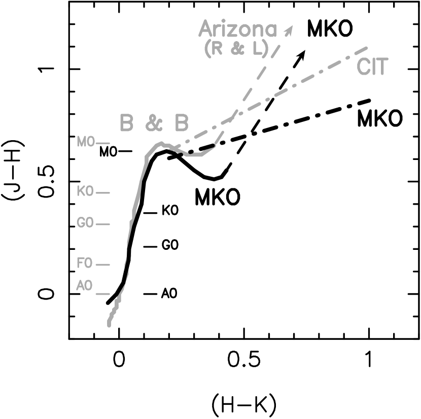
Figure 3.— Left: ($J-H$) vs. ($H-K$) diagram in the MKO photometric system. The dwarf star track (solid line) is constructed from colors of dwarf stars observed with MKO filters (Hewett et al. 2006, open circle, B9V–M6; Leggett et al. 2002, plus symbol, M4V–M6V; Leggett et al. 2006, cross symbol, M4–M6). See the details in the main text. CTTS locus (dot-dashed line) is estimated by least-square fit of the CTTS data (star symbol). The reddening vector for $A_{V}=5$ mag is shown with a dashed arrow from M6V location on the dwarf star track. Right: Comparison of dwarf star tracks (solid lines), CTTS loci (dot-dashed lines), and reddening vectors (dashed arrows) in MKO (black) and other photometric systems (gray). For the latter, the dwarf star track is in Johnson-Glass system (Bessel & Brett, 1988), the reddening vector is in Arizona system (Rieke & Lebofsky, 1985), and the CTTS locus is in CIT system (Meyer et al., 1997).

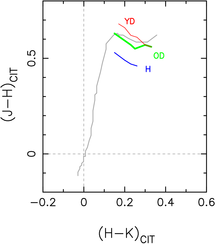
Figure 4.— Dwarf star tracks of differing metallicities in $JHK$ color-color diagram. Note that all the colors are shown in CIT system. Color lines are low-mass star tracks from Table 6 in Leggett (1992). YD ([M/H] $\sim 0.0$; M0–M6), OD ([M/H] $\sim-0.5$; M0–M5.5), and H ([M/H] $<-1.0$; K7–M3) represent stars in young disk, old disk, and halo, respectively. The gray line shows the standard dwarf track from Bessel & Brett (1988) after converting the color system from Johnson-Glass to CIT using the transformation in Leggett (1992).

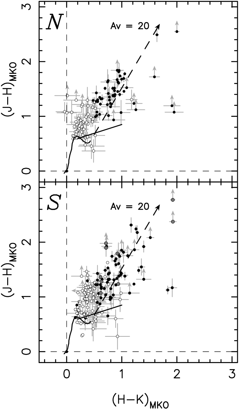
Figure 5.— ($J-H$) vs. ($H-K$) color-color diagrams of the Cloud 2-N cluster (top) and the Cloud 2-S cluster (bottom). Identified cluster members and field stars are shown with filled circles and open circles, respectively. Cloud 2-S sub-cluster members are shown with circled crosses (bottom). Only stars detected with more than $5\sigma$ in all $JHK$-bands are plotted. The dwarf star track, CTTS locus, and reddening vector are based on the MKO photometric system (see Fig. 3 and discussion in $\S$ 3, $\S$ 4). For stars that are not detected with 5 $\sigma$ in $J$-band, we showed the $J-H$ upper limit.

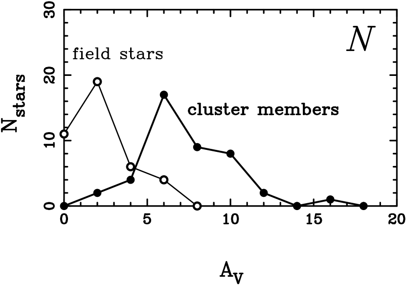
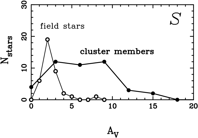
Figure 6.— $A_{V}$ distribution of Cloud 2 cluster members (thick lines) and field stars (thin lines). Average $A_{V}$ values of the members in Cloud 2-N and -S clusters are 7.2 and 6.1 mag, respectively, while those field stars in the Cloud 2-N and -S clusters are both 2.2 mag, respectively. Note that Cloud 2-S sub-cluster members are not counted in the right plot.

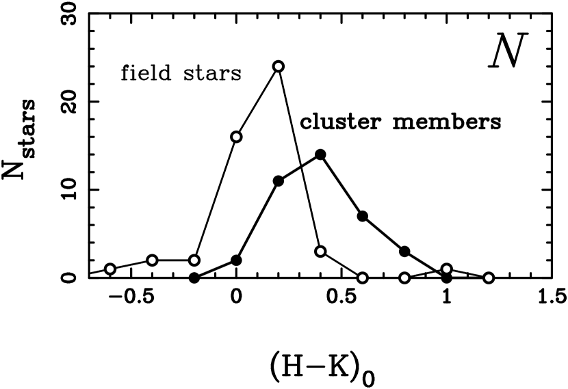
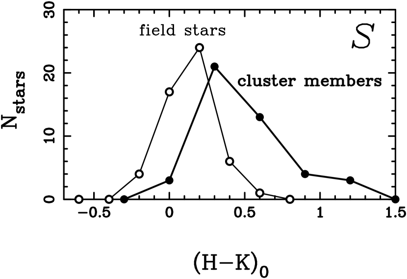
Figure 7.— $(H-K)_{0}$ distributions of Cloud 2 clusters’ members (thick lines) and field stars (thin lines). Average $(H-K)_{0}$ values of the cluster members in Cloud 2-N and Cloud 2-S clusters are 0.37 and 0.49 mag, respectively, while those field stars in Cloud 2-N and -S clusters are 0.11 and 0.12 mag, respectively.

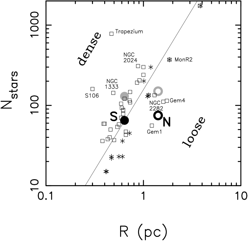
Figure 8.— $N_{\rm star}$ vs. cluster radius for the Cloud 2-N cluster (open circle), Cloud 2-S cluster (filled circle), plotted along with the data for nearby embedded clusters from Lada & Lada (2003, squares) and Carpenter (2000, stars). The solid line shows the constant stellar density of 50 pc^-2. The gray open and filled circles show the points for the Cloud 2 clusters for the case that all the stars are unresolved binaries.

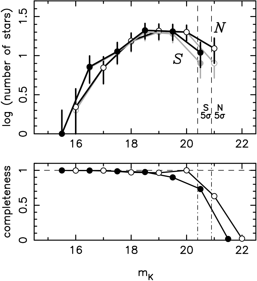
Figure 9.— Top: The raw KLF (gray lines) and completeness-corrected KLF (black lines) of Cloud 2 clusters. The observed KLFs for the Cloud 2-N and Cloud 2-S clusters are shown with filled circle and open circle, respectively. Error bars show the uncertainties due to Poisson statistics. Dashed lines show the limiting magnitudes of 5 $\sigma$ detection (Cloud 2-N: 20.9 mag, Cloud 2-S: 20.4 mag). Bottom: Detection completeness curves derived from the simulations using the artificial point sources. See the details in the main text.

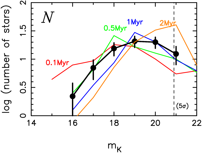
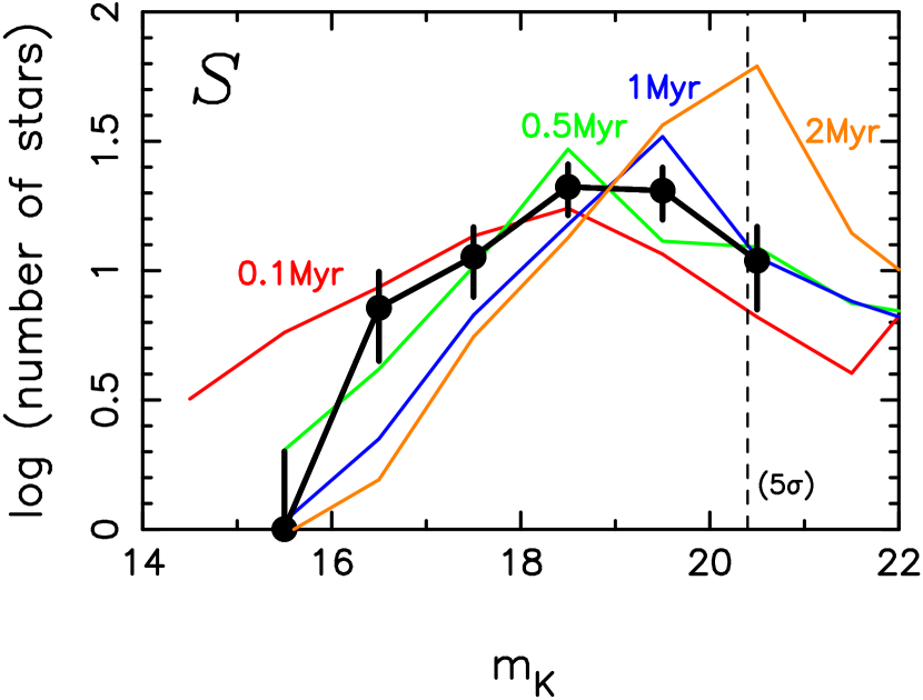
Figure 10.— Comparison of completeness-corrected KLF (thick line) with model KLFs of various ages (colored lines) for the Cloud 2-N cluster (left) and Cloud 2-S cluster (right). Red, green, blue, and orange lines represent the model KLFs of 0.1 Myr, 0.5 Myr, 1 Myr, and 2 Myr, respectively. The underlying IMF for the model KLFs is the Trapezium IMF by Muench et al. (2002).

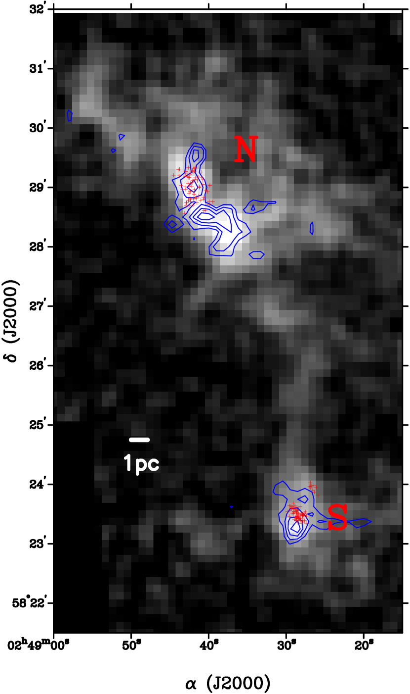
Figure 11.— Spatial distribution of Cloud 2 clusters (red crosses) and Cloud 2 cores (blue contour for ¹³CO and gray scale for ¹²CO from Saito et al. (2007)). The Cloud 2-N has two sub-peaks, while the Cloud 2-S core appears to be single core. The Cloud 2-N cluster seems to be associated only with northern core of the Cloud 2-N. The contour interval is 0.05 K km s^-1 and ranges from 0.20 to 0.45 K km s^-1 and the gray-scale range is from 0.0 to 1.7 K km s^-1. The temperature scale is in T${}_{\rm A}^{*}$. The beam size is about $19^{\prime\prime}$ for both ¹²CO and ¹³CO.

References

- Adams et al. (2006) Adams, F. C., Proszkow, E. M., Fatuzzo, M., & Myers, P. C. 2006, ApJ, 641, 504
- Allen et al. (2007) Allen, L., et al. 2007, Protostars and Planets V, B. Reipurth, D. Jewitt, and K. Keil (eds.), University of Arizona Press, Tucson, 951 pp., 2007., p.361-376, 361
- Arnault et al. (1988) Arnault, P., Knuth, D., Casoli, F., & Combes, F. 1988, A&A, 205, 41
- Baraffe et al. (2002) Baraffe, I., Chabrier, G., Allard, F., & Hauschildt, P. H. 2002, A&A, 382 563
- Baraffe et al. (1997) Baraffe, I., Chabrier, G., Allard, F., & Hauschildt, P. H. 1997, A&A, 327, 1054
- Bertin & Arnouts (1996) Bertin, E., & Arnouts, S. 1996, A&AS, 117, 393
- Bessel & Brett (1988) Bessell, M. S. & Brett, J. M. 1988, PASP, 100 1134
- Brand & Blitz (1993) Brand, J., & Blitz, L. 1993, A&A, 275, 67
- Brand & Wouterloot (1994) Brand, J., & Wouterloot, J. G. A. 1994, A&AS, 103, 503
- Brand & Wouterloot (1995) Brand, J., & Wouterloot, J. G. A. 1995, A&A, 303, 851
- Cambrésy et al. (2002) Cambrésy, L., Beichman, C. A., Jarrett, T. H., & Cutri, R. M. 2002, AJ, 123, 2559
- Carpenter (2000) Carpenter, J. M. 2000, AJ, 120, 3139
- D’Antona & Mazzitelli (1997) D’Antona, F., & Mazzitelli, I. 1997, Memorie della Societa Astronomica Italiana, 68, 807
- D’Antona & Mazzitelli (1998) D’Antona, F., & Mazzitelli, I. 1998, ASP Conf. Ser. 134: Brown Dwarfs and Extrasolar Planets, 134, 442
- Digel et al. (1994) Digel, S., de Geus E. J., & Thaddeus, P. 1994, ApJ, 422, 92.
- de Geus et al. (1993) de Geus, E. J., Vogel, S. N., Digel, S. W., & Gruendl, R. A. 1993, ApJ, 413, L97
- Fich & Blitz (1984) Fich, M., & Blitz, L. 1984, ApJ, 279, 125
- Girardi et al. (2002) Girardi, L., Bertelli, G., Bressan, A., Chiosi, C., Groenewegen, M. A. T., Marigo, P., Salasnich, B., & Weiss, A. 2002, A&A, 391, 195
- Haisch et al. (2001) Haisch, K. E., Jr., Lada, E. A., & Lada, C. J. 2001, ApJ, 553, L153
- Hartmann (2002) Hartmann, L. 2002, ApJ, 578, 914
- Hartmann et al. (2005) Hartmann, L., Megeath, S. T., Allen, L., Luhman, K., Calvet, N., D’Alessio, P., Franco-Hernandez, R., & Fazio, G. 2005, ApJ, 629, 881
- Heyer et al. (1998) Heyer, M. H., Brunt, C., Snell, R. L., Howe, J. E., Schloerb, F. P., & Carpenter, J. M. 1998, ApJS, 115, 241
- Hewett et al. (2006) Hewett, P. C., Warren, S. J., Leggett, S. K., & Hodgkin, S. T. 2006, MNRAS, 367, 454
- Ichikawa et al. (2006) Ichikawa, T., et al. 2006, Proc. SPIE, 6269,
- Kobayashi et al. (2000) Kobayashi, N. et al. 2000, Proc. SPIE, 4008, 1056
- Kobayashi et al. (2005) Kobayashi, N., Yasui, C., Tokunaga, A. T., & Saito, M. 2005, prpl. conf. 8639
- Kobayashi & Tokunaga (2000) Kobayashi, N., & Tokunaga, A. T. 2000, ApJ, 532, 423
- Kobayashi et al. (2007) Kobayashi, N., Yasui, C., Tokunaga, A. T., & Saito, M. 2007, submitted to ApJ
- Kroupa (2002) Kroupa, P. 2002, Science 295, 82
- Lada & Adams (1992) Lada, C. J., & Adams, F. C. 1992, ApJ, 393, 278
- Lada (1992) Lada, E. A. 1992, ApJ, 393, L25
- Lada et al. (1993) Lada, C. J., Young, E. T., & Greene, T. P. 1993, ApJ, 408, 471
- Lada et al. (1997) Lada, E. A., Evans, N. J., II, & Falgarone, E. 1997, ApJ, 488, 286
- Lada (1999) Lada, E. A. 1999. Lada, C.J. & Kylafis, N.D. eds. 1999, The Origin of Stars and Planetary Systems pp. 441-78
- Lada & Lada (2003) Lada, C. J., & Lada, E. A. 2003, ARA&A, 41, 57
- Lada et al. (2006) Lada, C. J., et al. 2006, AJ, 131, 1574
- Lada et al. (2000) Lada, C. J., Muench, A. A., Haisch, K. E., Jr., Lada, E. A., Alves, J. F., Tollestrup, E. V., & Willner, S. P. 2000, AJ, 120, 3162
- Leggett (1992) Leggett, S. K. 1992, ApJS, 82, 351
- Leggett et al. (2002) Leggett, S. K., et al. 2002, ApJ, 564, 452
- Leggett et al. (2006) Leggett, S. K., et al. 2006, MNRAS, 373, 781
- Lada et al. (1991a) Lada, E. A., Bally, J., & Stark, A. A. 1991a, ApJ, 368, 432
- Lada et al. (1991b) Lada, E. A., Evans, N. J., II, Depoy, D. L., & Gatley, I. 1991b, ApJ, 371, 171
- Lubowich et al. (2004) Lubowich, D. A., Brammer, G., Roberts, H., Millar, T. J., Henkel, C., & Pasachoff, J. M. 2004 oee sympE, 37L
- Meyer et al. (1997) Meyer, M. R., Calvet, N., & Hillenbrand, L. A. 1997, AJ, 114, 288
- Miller & Scalo (1979) Miller, G.E & Scalo, J.M. 1979, ApJS 41, 513
- Muench et al. (2000) Muench, A. A., Lada, E. A., & Lada, C. J. 2000, ApJ, 533, 358
- Muench et al. (2002) Muench, A. A., Lada, E. A., Lada, C. J., & Alves, J. 2002, ApJ, 573, 366
- Muzzio & Rydgren (1974) Muzzio, J. C., & Rydgren, A. E. 1974, AJ, 79, 864
- Nakajima et al. (2005) Nakajima, Y., et al. 2005, AJ, 129, 776
- Nakanishi & Sofue (2003) Nakanishi, H., & Sofue, Y. 2003, PASJ, 55, 191
- Nishiyama et al. (2006) Nishiyama, S., et al. 2006, ApJ, 638, 839
- Persson et al. (1998) Persson, S. E., Murphy, D. C., Krzeminski, W., Roth, M., & Rieke, M. J. 1998, AJ, 116, 2475
- Ridge et al. (2003) Ridge, N. A., Wilson, T. L., Megeath, S. T., Allen, L. E., & Myers, P. C. 2003, AJ, 126, 286
- Rieke & Lebofsky (1985) Rieke, G. H., & Lebofsky, M. J. 1985, ApJ, 288, 618
- Rudolph et al. (1996) Rudolph, A. L., Brand, J., de Geus, E. J., & Wouterloot, J. G. A. 1996, ApJ, 458, 653
- Ruffle et al. (2007) Ruffle, P. M. E., Millar, T. J., Roberts, H., Lubowich, D. A., Henkel, C., Pasachoff, J. M., Brammer, G., & . 2007, ArXiv e-prints, 708, arXiv:0708.2740
- Rolleston et al. (2000) Rolleston, W. R. J., Smartt, S. J., Dufton, P. L., & Ryans, R. S. I. 2000, A&A, 363, 537
- Saito et al. (2007) Saito, M., Kobayashi, N., Yasui, C., Tokunaga, A. T., & Sorai, K. 2007, in preparation
- Santos et al. (2000) Santos, C. A., Yun, J. L., Clemens, D. P., & Agostinho, R. J. 2000, ApJ, 540, 87
- Scalo (1998) Scalo, J. 1998, ASPC, 142, 201
- Siess et al. (2000) Siess, L., Dufour, E., & Forestini, M. 2000, A&A, 358, 593
- Sicilia-Aguilar et al. (2006) Sicilia-Aguilar, A., et al. 2006, ApJ, 638, 897
- Simons & Tokunaga (2002) Simons, D. A., & Tokunaga, A. 2002, PASP, 114, 169
- Smartt & Rolleston (1997) Smartt, S. J., & Rolleston, W. R. J. 1997, ApJ, 481, L47
- Smartt et al. (1996) Smartt, S. J., Dufton, P. L., & Rolleston, W. R. J. 1996, A&A, 305, 164
- Snell et al. (2002) Snell, R. L., Carpenter, J. M., & Heyer, M. H. 2002, ApJ, 578, 229
- Stephens & Leggett (2004) Stephens, D. C., & Leggett, S. K. 2004, PASP, 116, 9
- Strom et al. (1989) Strom, K. M., Strom, S. E., Edwards, S., Cabrit, S., & Skrutskie, M. F. 1989, AJ, 97, 1451
- Stil & Irwin (2001) Stil, J. M., & Irwin, J. A. 2001, ApJ, 563, 816.
- Terada et al. (2004) Terada, H., Kobayashi, N., Tokunaga, A. T., Pyo, T.-S., Nedachi, K, Weber, M, Potter, R., Onaka, P. M. 2004, Proc. SPIE, 5492, 1542
- Tokunaga et al. (2002) Tokunaga, A. T., Simons, D. A., & Vacca, W. D. 2002, PASP, 114, 180
- Tokunaga et al. (1998) Tokunaga, A. T., et al. 1998, Proc. SPIE, 3354, 512
- Yasui et al. (2006) Yasui, C., Kobayashi, N., Tokunaga, A. T., Terada, H., & Saito, M. 2006, ApJ, 649, 753
- Warin et al. (1996) Warin, S., Castets, A., Langer, W. D., Wilson, R. W., & Pagani, L. 1996, A&A, 306, 935
- Westerhout & Wendlandt (1982) Westerhout, G., & Wendlandt, H.-U. 1982, A&AS, 49, 143
- Wouterloot & Brand (1989) Wouterloot, J. G. A., & Brand, J. 1989, A&AS, 80, 149