Kernel Convergence Estimates for Diffusions with Continuous Coefficients

Abstract.

We are interested in the kernel of one-dimensional diffusion equations with continuous coefficients as evaluated by means of explicit discretization schemes of uniform step $h>0$ in the limit as $h\to 0$. We consider both semidiscrete triangulations with continuous time and explicit Euler schemes with time step small enough for the method to be stable. We find sharp uniform bounds for the convergence rate as a function of the degree of smoothness which we conjecture. The bounds also apply to the time derivative of the kernel and its first two space derivatives. Our proof is constructive and is based on a new technique of path conditioning for Markov chains and a renormalization group argument. Convergence rates depend on the degree of smoothness and Hölder differentiability of the coefficients. We find that the fastest convergence rate is of order $O(h^{2})$ and is achieved if the coefficients have a bounded second derivative. Otherwise, explicit schemes still converge for any degree of Hölder differentiability except that the convergence rate is slower. Hölder continuity itself is not strictly necessary and can be relaxed by an hypothesis of uniform continuity.

1. Introduction and Notations

Consider a pair of backward and forward one-dimensional diffusion equations of the form

(1.1) $${\partial\over\partial t}f(x;t)+{\mathcal{L}}^{0}_{x}f(x;t)=0,\;\;\;\;\;\;\;\;\;\;{\partial\over\partial t}g(y;t)={\mathcal{L}}^{0*}_{y}g(y;t)$$

where

(1.2) $${\mathcal{L}}^{0}_{x}={1\over 2}{\sigma(x)^{2}}{\partial^{2}\over\partial x^{2}}+\mu(x){\partial\over\partial x}.$$

and its adjoint formally acts as follows:

(1.3) $$({\mathcal{L}}^{0*}_{y}\phi)(y)={1\over 2}{\partial^{2}\over\partial y^{2}}\big{(}\sigma(y)^{2}\phi(y)\big{)}+{\partial\over\partial y}\big{(}\mu(y)\phi(y)\big{)}.$$

on a test function $\phi$. These equations are defined on the bounded interval $A=[-L,L]\subset{\mathbb{R}}$ where $0<L<\infty$. For simplicity, we assume periodic boundary conditions and identify the two boundary points $\pm L$ with each other.

In most of the paper, the coefficients $\sigma(x)$ and $\mu(x)$ are assumed to be Hölder differentiable. More precisely, if $\alpha\in(0,1]$, $k\in{\mathbb{N}}$ where ${\mathbb{N}}=\{0,1,...\}$ and the function $\phi(x)\in\mathcal{C}^{k}(A)$ has $k\geq 1$ continuous derivatives, then one says that $\phi$ is Hölder differentiable of order $(k,\alpha)$ if there exists a constant $c>0$ such that

(1.4) $$\big{\lvert}\phi^{(k)}(x)-\phi^{(k)}(y)\big{\lvert}\leq cd(x,y)^{\alpha}\;\;\;\;$$

uniformly for all $x,y\in A$. In case $k=0$ the function is called Hölder continuous. The distance is defined consistently with the assumed periodic boundary conditions and is given by

(1.5) $$d(x,y)=\min_{n}\lvert x-y-2Ln\lvert.$$

The linear space of Hölder continuous or Hölder differentiable periodic functions of order $(k,\alpha)$ on $A$ is denoted with $\mathcal{C}^{k,\alpha}(A)$. We are interested in the case where $\sigma^{2}\in\mathcal{C}^{k,\alpha}(A)$ and $\mu\in\mathcal{C}^{j,\beta}(A)$ with $k+\alpha>0$ and $j+\beta>0$.

The hypothesis of Hölder continuity can be relaxed slightly by assuming uniform continuity instead, i.e. that both $\sigma(x)^{2}$ and $\mu(x)$ satisfy a bound of the form

(1.6) $$\big{\lvert}\phi(x)-\phi(y)\big{\lvert}\leq c\rho\big{(}d(x,y)\big{)}\;\;\;\;$$

where $\rho(d)$ is a non-decreasing function such that $\lim_{d\downarrow 0}\rho(d)=0$.

Let $u_{0}(x,y;t)$ denote a kernel of equation (1.17), i.e. a weak solution of the forward equation

(1.7) $${\partial\over\partial t}u_{0}(x,y;t)={\mathcal{L}}^{0*}_{y}u_{0}(x,y;t)$$

where the operator ${\mathcal{L}}^{0*}_{y}$ acts on the $y$ coordinate and the following initial time condition is satisfied:

(1.8) $$\lim_{t\downarrow 0}u_{0}(x,y;t)=\delta(x-y).$$

The kernel $u_{0}(x,y;t)$ formally satisfies also the backward equation

(1.9) $${\partial\over\partial t}u_{0}(x,y;t)+{\mathcal{L}}^{0}_{x}u_{0}(x,y;t)=0$$

where the operator ${\mathcal{L}}^{0}_{x}$ acts on the $x$ coordinate.

We are interested in existence, uniqueness, smoothness and approximation schemes for the kernel $u_{0}(x,y;t)$, its first two space derivatives with respect to the $x$ variable and its first time derivative $\partial_{t}u_{0}(x,y;t)$. As a byproduct of this analysis, we also find conclusions about the convergence of ${\mathcal{L}}^{0}_{x}u_{0}(x,y;t)$ and ${\mathcal{L}}^{0*}_{y}u_{0}(x,y;t)$, as both expressions equal the first time derivative.

Diffusion equations are one of the single most studied topics in the literature. Existence and uniqueness questions for the kernel were address in [Kolmogorov1931], [Feller1936], [Hille], [Yosida] and [Ito57]. A classification of all the possible boundary conditions is in [Feller52]. The case of Hölder continuous coefficients was resolved in [Philips] based on methods in [Friedrichs] and [LaxPhilips]. The hypothesis of Hölder continuity was relaxed to uniform continuity in [FabesRiviere] and [SV1969]. Strook and Varadhan also introduce a new probabilistic framework where existence is proved by reduction to the so-called martingale problem and a compactness argument, thus shifting the attention from the kernel itself to the underlying measure space.

The existence of a weak limit of continuous time Markov chains as $h_{m}\downarrow 0$ was established in [Sova] and [Kurtz] by using operator semigroup methods, see also the book [EthierKurtz] for a review. Convergence in the semigroup sense takes place if the limit

(1.10) $$(T_{t}\phi)(x)=\lim_{m\to\infty,m\geq n}\sum_{y\in h_{m}Z\cap A}u_{h_{m}}(x,y;t)\phi(y)$$

exists for all test functions $\phi\in{\mathcal{C}}^{\infty}(A)$, uniformly for all $x\in A_{n},n\geq 0$. A key result is that a necessary and sufficient condition for this limit to exist and define a semigroup $T_{t}$ is that generators converge also in the same Banach space, i.e. that also the limit

(1.11) $$\lim_{h_{m}\downarrow 0}{\mathcal{L}}^{h_{m}}_{x}\phi={\mathcal{L}}^{0}_{x}\phi$$

exists in the uniform norm for all test functions $\phi\in{\mathcal{C}}^{\infty}(A)$. See [EthierKurtz] for a precise statement with all the technical conditions and a proof. In [SV] convergence is reconsidered again by reduction to the martingale problem.

The problem has also been studied extensively in the numerical analysis literature. Explicit and implicit Euler schemes where coefficients are smooth and the data is rough in the sense that it belongs to a $L^{2}$ space have been considered by several authors. In the case that the Markov generator is symmetric and time independent, one can make use of a spectral representation as in [BakerBrambleThomte] and with greater effort such methods may also be used for more general situations, see [Suzuki]. In [LuskinRannacher], a parabolic duality argument is used to show convergence for the standard Galerkin method. [MingyouThomee] use a simpler argument based on energy estimates. In [Palencia] one finds convergence bounds in maximum norm assuming the initial condition is uniformly bounded and coefficients are constant.

In this article, we revisit this classic theme by considering the problem of obtaining the kernel constructively as a limit of increasingly fine triangulations schemes and in assessing the rate of convergence with pointwise bounds on the kernel itself. More precisely, let $h_{m}=L2^{-m},m\in{\mathbb{N}}$ and let $A_{m}{h_{m}}{\mathbb{Z}}\cap A$. Consider the sequence of operators

(1.12) $${\mathcal{L}}^{m}_{x}={\sigma(x)^{2}\over 2}\Delta^{m}_{x}+\mu(x)\nabla^{m}_{x}.$$

defined on the $2^{m+1}$-dimensional space of all periodic functions $f_{m}:A_{m}\to{\mathbb{R}}$, where

(1.13) $$\nabla^{m}_{x}f(x)={f(x+{h_{m}})-f(x-{h_{m}})\over 2{h_{m}}}.$$

and

(1.14) $$\Delta^{m}_{x}f(x)={f(x+{h_{m}})+f(x-{h_{m}})-2f(x)\over{h_{m}}^{2}}$$

These definitions also apply to the boundary points by periodicity. We assume that $m\geq m_{0}$ where $m_{0}$ is the least integer such that

(1.15) $${\sigma^{2}(x)\over 2h_{m}^{2}}>{\lvert\mu(x)\lvert\over 2h_{m}}$$

for all $m\geq m_{0}$ and all $x\in A_{m}$.

Let $u_{m}(x,y;t)$ denote the kernel of equation (1.17), i.e. the solution of the (forward) equation

(1.16) $${\partial\over\partial t}u_{m}(x,y;t)={\mathcal{L}}^{m*}_{y}u_{m}(x,y;t)$$

where the operator ${\mathcal{L}}^{m*}_{y}$ acts on the $y$ coordinate and the following initial time condition is satisfied:

(1.17) $$\lim_{t\downarrow 0}u_{m}(x,y;t)=\delta_{m}(x-y).$$

Here,

(1.18) $$\delta_{m}(x-y)=\begin{cases}{1\over h_{m}}\;\;\;\;\;\;\;{\rm if}\;\;x=y\;\;\;{\rm mod}\;2L\\ 0\;\;\;\;\;\;\;\;\;{\rm otherwise}.\end{cases}$$

Since (1.17) is a finite system of linear ordinary differential equations, the solution exists and is unique for all times. The kernel $u_{m}(x,y;t)$ satisfies also the backward equation

(1.19) $${\partial\over\partial t}u_{m}(x,y;t)+{\mathcal{L}}^{m}_{x}u_{m}(x,y;t)=0$$

where the operator ${\mathcal{L}}^{m}_{x}$ acts on the $x$ coordinate. Using functional calculus notations for the exponential of a matrix, we also have that

(1.20) $$u_{m}(x,y;t)={1\over h_{m}}\exp\big{(}t{\mathcal{L}}^{m}\big{)}(x,y).$$

Our main result can be stated as follows:

Theorem 1.

Suppose that $\sigma^{2}\in{\mathcal{C}}^{k,\alpha}$ and $\mu\in{\mathcal{C}}^{j,\beta}$ and let

(1.21) $$\gamma=\min\{2,k+\alpha,j+\beta\}.$$

Assume that $\gamma>0$. Then there is a constant $c>0$ such that for all $m^{\prime}\geq m\geq m_{0}$ and all $x,y\in A_{m}$ the following inequalities hold:

• (1.22) $$\lvert u_{m}(x,y;t)-u_{m^{\prime}}(x,y;t)\lvert\leq ch_{m}^{\gamma}$$

• $$\lvert\partial_{t} u_{m}(x,y;t)-\partial_{t}u_{m^{\prime}}(x,y;t)\lvert$$

  $$=\lvert{\mathcal{L}}^{m*}_{y}u_{m}(x,y;t)-{\mathcal{L}}^{m^{\prime}*}_{y}u_{m^{\prime}}(x,y;t)\lvert$$

  $$=\lvert{\mathcal{L}}^{m}_{x}u_{m}(x,y;t)-{\mathcal{L}}^{m^{\prime}}_{x}u_{m^{\prime}}(x,y;t)\lvert\leq ch_{m}^{\gamma}.$$

A version of this theorem under slightly weaker conditions can be formulated as follows:

Theorem 2.

Suppose that $\sigma(x)^{2}$ and $\mu(x)$ are uniformly continuous functions in $A$. Let the function $\rho(d)$ be non-decreasing and be such that $\lim_{d\downarrow 0}\rho(d)=0$ and equation (1.6) holds. Then there is a constant $c>0$ such that for all $m^{\prime}\geq m\geq m_{0}$ and all $x,y\in A_{m}$ the following inequalities hold:

• (1.24) $$\lvert u_{m}(x,y;t)-u_{m^{\prime}}(x,y;t)\lvert\leq c\rho(h_{m})$$

• $$\lvert\partial_{t} u_{m}(x,y;t)-\partial_{t}u_{m^{\prime}}(x,y;t)\lvert$$

  $$=\lvert{\mathcal{L}}^{m*}_{y}u_{m}(x,y;t)-{\mathcal{L}}^{m^{\prime}*}_{y}u_{m^{\prime}}(x,y;t)\lvert$$

  $$=\lvert{\mathcal{L}}^{m}_{x}u_{m}(x,y;t)-{\mathcal{L}}^{m^{\prime}}_{x}u_{m^{\prime}}(x,y;t)\lvert\leq c\rho(h_{m}).$$

Next, we consider the case where also time is discretized and prove the following result:

Theorem 3.

Suppose that $\sigma^{2}$ and $\mu$ satisfy equations of the form (1.6) with a non-decreasing function $\rho(d)$ such that $\lim_{d\downarrow 0}\rho(d)=0$. Consider the discretized kernel

(1.26) $$u^{\delta t}_{m}(x,y;t)=h_{m}^{-1}\left(1+\delta t{\mathcal{L}}^{m}\right)^{t\over\delta t}(x,y;t).$$

where ${\mathcal{L}}^{m}$ is the operator in (1.12) and $\delta t_{m}$ is so small that

(1.27) $$\min_{x\in A_{m}}1+\delta t_{m}{\mathcal{L}}^{m}(x,x)>0$$

Assume that boundary conditions are periodic and that the ratio ${t\over\delta t}=N$ is an integer. Then here is a constant $c>0$ such that the following bounds hold for all $m\geq m_{0}$ and all $x,y\in A_{m}$:

• (1.28) $$\lvert u_{m}(x,y;t)-u_{m}^{\delta t}(x,y;t)\lvert\leq ch_{m}^{2}$$

• $$\bigg{\lvert}\partial_{t} u_{m}(x,y;t)-{u_{m}^{\delta t}(x,y;t+\delta t)-u_{m}^{\delta t}(x,y;t)\over\delta t}\bigg{\lvert}$$

  $$=\lvert{\mathcal{L}}^{m*}_{y}u_{m}(x,y;t)-{\mathcal{L}}^{m*}_{y}u_{m}^{\delta t}(x,y;t)\lvert$$

  $$=\lvert{\mathcal{L}}^{m*}_{x}u_{m}(x,y;t)-{\mathcal{L}}^{m*}_{x}u_{m}^{\delta t}(x,y;t)\lvert\leq ch^{2}$$

The paper is organized as follows. In Section 2 we consider the case of Brownian motion and review a result in [AlbaneseMijatovicBM] which establishes the theorems above in this simple particular case where Fourier analysis in the space direction can be used to carry out a precise calculation. In Section 3, we consider the case of a diffusion where both the volatility and the drift have two bounded derivatives. In this case, we make use of time-homogeneity and carry out a Fourier transform in the time direction after path conditioning. In Section 4, we extend the derivation to the case of non-smooth coefficients. Section 5 is dedicated to the case where time is discretized and we prove Theorem 3.

2. Constant Coefficients

In this Section, we prove Theorem 1 in the special case where the volatility and the drift coefficients are constant, i.e.

(2.1) $${{\mathcal{L}}^{m}}_{x}=\mu\nabla^{m}_{x}+{1\over 2}\sigma^{2}\Delta^{m}_{x}.$$

It suffices to consider the case $m^{\prime}=m+1$. Let $B_{m}$ be the Brillouin zone defined as follows:

(2.2) $$B_{m}=\left\{-{2^{m-1}\pi\over L}+{k\pi\over L},k=0,..2^{m}-1\right\}$$

Let ${\mathcal{F}}_{m}:\ell^{2}(A_{m})\to\ell^{2}(B_{m})$ be the Fourier transform operator defined so that:

(2.3) $$\hat{f}(p)\equiv{\mathcal{F}}_{m}(f)(p)=h_{m}\sum_{x\in A_{m}}f(x)e^{-ipx}$$

for all $p\in B_{m}$. The inverse Fourier transform is given by

(2.4) $${\mathcal{F}}_{m}^{-1}(\hat{f})(x)={1\over 2L}\sum_{p\in B_{m}}\hat{f}(p)e^{ipx}.$$

The Fourier transformed generator is diagonal and is given by the operator of multiplication by

(2.5) $$\hat{\ell}^{m}(p)={\mathcal{F}}_{m}{{\mathcal{L}}^{m}}{\mathcal{F}}_{m}^{-1}(p,p)=-i\mu{\sin h_{m}p\over h_{m}}+{\sigma^{2}}{\cos h_{m}p-1\over h_{m}^{2}}.$$

We have

(2.6) $$u_{m}(x,y;t)={1\over 2L}\sum_{p\in B_{m}}e^{t\hat{\ell^{m}}(p)}e^{ip(y-x)}.$$

Using this Fourier series representation, we find

$$\big{\lvert}u_{m}(x,y;t)-u_{m+1}(x,y;t)\big{\lvert}$$

$$\leq{1\over 2L}\bigg{\lvert}\sum_{p\in B_{m}}\bigg{(}e^{t{\hat{\ell}^{m}}(p)}-e^{t{\hat{\ell}^{m+1}}(p)}\bigg{)}e^{ip(y-x)}\bigg{\lvert}+{1\over 2L}\bigg{\lvert}\sum_{p\in B_{m+1}\setminus B_{m}}e^{t{\hat{\ell}^{m+1}}(p)}e^{ip(y-x)}\bigg{\lvert}.$$

Let

(2.8) $$K_{m}=\sqrt{\lvert\log h_{m+1}\lvert\over\sigma^{2}t}.$$

If $h_{m}$ is small enough, i.e. if $m_{0}$ is sufficiently large, we have that

$${1\over 2L}\bigg{\lvert}\sum_{p\in B_{m},\lvert p\lvert\geq K_{m}}e^{t{\hat{\ell}^{m}}(p)}e^{ip(y-x)}\bigg{\lvert}\leq{1\over 2L}\sum_{p\in B_{m},\lvert p\lvert\geq K_{m}}e^{t\Re(\hat{\ell}^{m}(p))}\leq c\exp\bigg{(}t\sigma^{2}{\cos h_{m}K_{m}-1\over h_{m}^{2}}\bigg{)}\leq ch_{m}^{2}.$$

where $\Re(a)$ denotes the real part of $a\in{\mathbb{C}}$ and $c$ denotes a generic constant. Similarly

$${1\over 2L}\bigg{\lvert}\sum_{p\in B_{m+1},\lvert p\lvert\geq K_{m}}e^{t{\hat{\ell}^{m+1}}(p)}e^{ip(y-x)}\bigg{\lvert}\leq{1\over 2L}\sum_{p\in B_{m},\lvert p\lvert\geq K_{m}}e^{t\Re(\hat{\ell}^{m+1}(p))}$$

$$\leq c\exp\bigg{(}t\sigma^{2}{\cos h_{m+1}K-1\over h_{m+1}^{2}}\bigg{)}\leq ch_{m+1}^{2}$$

Since

(2.11) $${1\over 2}h^{2}p^{3}-{1\over 8}h^{4}p^{5}\leq{\sin hp\over h}-{\sin 2hp\over 2h}\leq{1\over 2}h^{2}p^{3}$$

and

(2.12) $$-{1\over 8}h^{2}p^{4}\leq{\cos hp-1\over h^{2}}-{\cos 2hp-1\over(2h)^{2}}\leq-{1\over 8}{h^{2}p^{4}}+{1\over 48}h^{4}p^{6}.$$

we find that if $\lvert p\lvert\leq{\sqrt{2}\over h}$ then

(2.13) $$\lvert\hat{\ell}^{m}(p)-\hat{\ell}^{m+1}(p)\lvert\leq{\mu\over 4}h^{2}\lvert p\lvert^{3}+{\sigma^{2}\over 16}h^{2}p^{4}.$$

Moreover, since

(2.14) $$-{1\over 2}p^{2}\leq{\cos hp-1\over h}\leq-{1\over 2}p^{2}+{1\over 24}h^{2}p^{4}$$

we conclude that in case $\lvert p\lvert\leq h^{-1}\sqrt{2\over 3}$, the following inequality holds:

(2.15) $${\cos hp-1\over h}\leq-{1\over 4}{p^{2}}$$

Hence, if $m_{0}$ is large enough, we find

$${1\over 2L}\bigg{\lvert}\sum_{p\in B_{m},\lvert p\lvert\leq K}\bigg{(}e^{t{\hat{\ell}^{m}}(p)}- e^{t{\hat{\ell}^{m+1}}(p)}\bigg{)}e^{ip(y-x)}\bigg{\lvert}$$

$$\leq{1\over 2L}\sum_{p\in B_{m},\lvert p\lvert\leq K}e^{-{1\over 4}{p^{2}}}\bigg{(}e^{{\mu t\over 4}h_{m}^{2}\lvert p\lvert^{3}+{\sigma^{2}t\over 16}h_{m}^{2}p^{4}}-1\bigg{)}$$

(2.16) $$\leq{1\over 2L}\sum_{p\in B_{m},\lvert p\lvert\leq K}e^{-{1\over 4}{p^{2}}}\bigg{(}{\mu t\over 4}h_{m}^{2}\lvert p\lvert^{3}+{\sigma^{2}t\over 16}h_{m}^{2}p^{4}\bigg{)}\leq ch_{m}^{2}$$

for some constant $c>0$ independent of $m$. This concludes the proof of convergence for the kernel in the special case of constant coefficients.

To estimate the first derivative, notice that

(2.17) $$\nabla u_{m}(x,y;t)={1\over L}\sum_{p\in B_{m}}e^{t\hat{\ell^{m}}(p)}{\sin ph_{m}\over h_{m}}e^{ip(y-x)}.$$

and

$$\big{\lvert}u_{m}(x,y;t)-u_{m+1}(x,y;t)\big{\lvert}$$

$$\leq{1\over 2L}\bigg{\lvert}\sum_{p\in B_{m}}\bigg{(}e^{t{\hat{\ell}^{m}}(p)}{\sin ph_{m}\over h_{m}}-e^{t{\hat{\ell}^{m+1}}(p)}{\sin ph_{m+1}\over h_{m+1}}\bigg{)}e^{ip(y-x)}\bigg{\lvert}$$

$$+{1\over 2L}\bigg{\lvert}\sum_{p\in B_{m+1}\setminus B_{m}}e^{t{\hat{\ell}^{m+1}}(p)}e^{ip(y-x)}\bigg{\lvert}.$$

Let

(2.19) $$K_{m}=2\sqrt{\lvert\log h_{m+1}\lvert\over\sigma^{2}t}.$$

If $h_{m}$ is small enough, we have that

$${1\over 2L}\bigg{\lvert}\sum_{p\in B_{m},\lvert p\lvert\geq K_{m}}e^{t{\hat{\ell}^{m}}(p)}{\sin ph_{m}\over h_{m}}e^{ip(y-x)}\bigg{\lvert}\leq{1\over 2L}\sum_{p\in B_{m},\lvert p\lvert\geq K_{m}}e^{t\Re(\hat{\ell}^{m}(p))}{\sin ph_{m}\over h_{m}}$$

$$\hskip 113.81102pt\leq c\bigg{\lvert}{\sin Kh_{m}\over h_{m}}\bigg{\lvert}\exp\bigg{(}t\sigma^{2}{\cos Kh_{m}-1\over h_{m}^{2}}\bigg{)}\leq ch_{m}^{2}.$$

where $c$ denotes a generic constant. Similarly

(2.21) $${1\over 2L}\bigg{\lvert}\sum_{p\in B_{m+1},\lvert p\lvert\geq K_{m}}e^{t{\hat{\ell}^{m+1}}(p)}e^{ip(y-x)}\bigg{\lvert}\leq ch^{2}.$$

If $m$ is large enough, we also find

$${1\over 2L}\bigg{\lvert} \sum_{p\in B_{m},\lvert p\lvert\leq K_{m}}\bigg{(}{\sin ph_{m}\over h_{m}}e^{t{\hat{\ell}^{m}}(p)}-{\sin ph_{m+1}\over h_{m+1}}e^{t{\hat{\ell}^{m+1}}(p)}\bigg{)}e^{ip(y-x)}\bigg{\lvert}$$

$$\leq{1\over 2L}\sum_{p\in B_{m},\lvert p\lvert\leq K_{m}}\bigg{\lvert}{\sin ph_{m}\over h_{m}}\bigg{\lvert}e^{-{1\over 4}{p^{2}}}\bigg{(}e^{{\mu t\over 4}h_{m}^{2}\lvert p\lvert^{3}+{\sigma^{2}t\over 16}h_{m}^{2}p^{4}}-1\bigg{)}$$

$$+e^{-{1\over 4}{p^{2}}}\bigg{\lvert}{\sin ph_{m+1}\over h_{m+1}}-{\sin ph_{m}\over h_{m}}\bigg{\lvert}\leq ch_{m}^{2}$$

for some constant $c>0$ independent of $m$. This concludes the proof of the bound of the first derivative. The second derivative can be derived in a similar way.

Finally, consider the following Fourier representation for the discretized kernel

(2.23) $$u_{m}^{\delta t}(x,y;t)={1\over L}\sum_{p\in B_{m}}\bigg{(}1+\delta t\hat{\ell^{m}}(p)\bigg{)}^{t\over\delta t}e^{ip(y-x)}.$$

Consider the formula

(2.24) $$\bigg{(}1+\delta t\hat{\ell^{m}}(p)\bigg{)}^{t\over\delta t}=\exp\bigg{(}t\log\big{(}1+\hat{\ell^{m}}(p)\big{)}\bigg{)}.$$

and let’s represent the difference between the discrete and continuous time kernels as follows:

$$\lvert u_{m}(x,y;t)-u_{m}^{\delta t}(x,y;t)\lvert$$

$$\leq{1\over 2L}\bigg{\lvert}\sum_{p\in B_{m}}\bigg{(}\exp\big{(}t{\hat{\ell}^{m}}(p)\big{)}-\exp\bigg{(}{t\over\delta t}\log\big{(}1+\delta t{\hat{\ell}}^{m}(p)\big{)}\bigg{)}e^{ip(y-x)}\bigg{\lvert}$$

$$\leq{1\over 2L}\sum_{p\in B_{m},p\leq K_{m}}e^{-{1\over 4}p^{2}}\bigg{\lvert}\exp\bigg{(}{t\over\delta t}\log\big{(}1+\delta t{\hat{\ell}}^{m}(p)\big{)}-t{\hat{\ell}^{m}}(p)\bigg{)}-1\bigg{\lvert}$$

$$\hskip 28.45274pt{1\over 2L}\sum_{p\in B_{m},p\geq K_{m}}\bigg{\lvert}\exp\big{(}t{\hat{\ell}^{m}}(p)\big{)}\bigg{\lvert}+{1\over 2L}\sum_{p\in B_{m},p\geq K_{m}}\bigg{\lvert}\exp\bigg{(}{t\over\delta t}\log\big{(}1+\delta t{\hat{\ell}}^{m}(p)\big{)}\bigg{)}\bigg{\lvert}$$

where $K_{m}$ is chosen as in (2.8). The very same bounds above lead to the conclusion that this difference is $\leq ch_{m}^{2}$.

3. Smooth Coefficients

In this section, we prove Theorem 1 in the case where the drift and volatility are both of class ${\mathcal{C}}^{(3,0)}$, i.e. they depend smoothly on the space coordinate but not on the time coordinate.

Let us introduce the following two constants characterizing the volatility function:

(3.1) $$\Sigma_{0}=\inf_{x\in A_{m}}\sigma(x),\;\;\;\;\;\Sigma_{1}=\sup_{x\in A_{m}}\sqrt{\sigma(x)^{2}+h_{m}\lvert\mu(x)\lvert}.$$

and let

(3.2) $$M=\sup_{x\in A_{m}}\lvert\mu(x)\lvert.$$

Since our interval is bounded, we have that $\Sigma_{0}>0$ and $\Sigma_{1},M<\infty$.

A symbolic path $\gamma=\{\gamma_{0},\gamma_{1},\gamma_{2},....\}$ is an infinite sequence of sites in $A_{m}$ such that $\gamma_{j}\neq\gamma_{j-1}$ for all $j=1,...$. Let $\Gamma_{m}$ be the set of all symbolic paths in $A_{m}$. The kernel of the diffusion process admits the following representation in terms of a summation over symbolic paths

(3.3) $$u_{m}(x,y;t)= {1\over h_{m}}\sum_{q=1}^{\infty}2^{-q}\sum_{\begin{matrix}\gamma\in\Gamma_{m}:\gamma_{0}=x,\gamma_{q}=y\\ \lvert\gamma_{j}-\gamma_{j-1}\lvert=1\;\;\forall j\geq 1\end{matrix}}W_{m}(\gamma,q,t)$$

where

(3.4) $$W_{m}( \gamma,q,t)={1\over h_{m}}\int_{0}^{t}ds_{1}\int_{s_{1}}^{t}ds_{2}...\int_{s_{q-1}}^{t}ds_{q}e^{(t-s_{q}){\mathcal{L}}_{m}(\gamma_{q},\gamma_{q})}\prod_{j=0}^{q-1}\bigg{(}e^{(s_{j+1}-s_{j}){\mathcal{L}}_{m}(\gamma_{j},\gamma_{j})}2{\mathcal{L}}_{m}(\gamma_{j},\gamma_{j+1})\bigg{)}$$

with $s_{0}=0$.

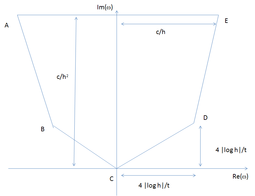
Figure 1. Contour of integration for the integral in (3.52). ${\mathcal{C}}_{+}$ is the countour joining the point $D$ to the points $E,A,B$. ${\mathcal{C}}_{-}$ is the countour joining the point $B$ to $C$ to $D$.

Let us introduce the following Green’s function:

(3.5) $$G_{m}(x,y;\omega)=\int_{0}^{\infty}u_{m}(x,y;t)e^{-i\omega t}dt=h_{m}^{-1}{1\over{\mathcal{L}}^{m}+i\omega}(x,y).$$

The propagator can be expressed as the following contour integral

(3.6) $$u_{m}(x,y;t)=\int_{{\mathcal{C}}_{-}}{d\omega\over 2\pi}G_{m}(x,y;\omega)e^{i\omega t}+\int_{{\mathcal{C}}_{+}}{d\omega\over 2\pi}G_{m}(x,y;\omega)e^{i\omega t}.$$

Here, ${\mathcal{C}}_{+}$ is the contour joining the point $D$ to the points $E,A,B$ in Fig. 1, while ${\mathcal{C}}_{-}$ is the contour joining the point $B$ to $C$ to $D$. By design, each point $\omega$ on the upper path ${\mathcal{C}}_{+}$ is separated from the spectrum of $\mathcal{L}$.

Lemma 1.

For $m$ sufficiently large, there is a constant $c>0$ such that

(3.7) $$\bigg{\lvert}\int_{{\mathcal{C}}_{+}}{d\omega\over 2\pi}G_{m}(x,y;\omega)e^{i\omega t}\bigg{\lvert}\leq ch^{2}.$$

Proof.

The proof is based on the geometric series expansion

(3.8) $$G_{m}(\omega)=h_{m}^{-1}{1\over{\mathcal{L}}^{m}+i\omega}=h_{m}^{-1}\sum_{j=0}^{\infty}{1\over{1\over 2}\sigma^{2}\Delta^{m}+i\omega}\bigg{[}\mu\nabla^{m}{1\over{1\over 2}\sigma^{2}\Delta^{m}+i\omega}\bigg{]}^{j}$$

whose convergence for $\omega\in{\mathcal{C}}_{+}$ can be established by means of a Kato-Rellich relative bound, see [Kato]. More precisely, for any $\alpha>0$, one can find a $\beta>0$ such that the operators $\nabla^{m}$ and $\Delta^{m}$ satisfy the following relative bound estimate:

(3.9) $$\lvert\lvert\nabla^{m}f\lvert\lvert_{2}\leq\alpha\lvert\lvert\Delta^{m}f\lvert\lvert_{2}+\beta\lvert\lvert f\lvert\lvert_{2}.$$

for all periodic functions $f$ and all $m\geq m_{0}$. This bound can be derived by observing that $\nabla^{m}$ and $\Delta^{m}$ can be diagonalized simultaneously by a Fourier transform, as done in the previous section, and by observing that for any $\alpha>0$, one can find a $\beta>0$ such that

(3.10) $$\bigg{\lvert}{\sin h_{m}p\over h_{m}}\bigg{\lvert}\leq\alpha\bigg{\lvert}{\cos h_{m}p-1\over h_{m}^{2}}\bigg{\lvert}+\beta$$

for all $m\geq m_{0}$ and all $p\in B_{m}$.

Under the same conditions, we also have that

(3.11) $$\big{\lvert}\big{\lvert}\mu\nabla^{m}f\big{\lvert}\big{\lvert}_{2}\leq{2M\alpha\over\Sigma_{0}^{2}}\bigg{\lvert}\bigg{\lvert}{1\over 2}\sigma^{2}\Delta^{m}f\bigg{\lvert}\bigg{\lvert}_{2}+\beta\lvert\lvert f\lvert\lvert_{2}.$$

Hence

(3.12) $$\bigg{\lvert}\bigg{\lvert}\mu\nabla^{m}{1\over{1\over 2}\sigma^{2}\Delta^{m}+i\omega}f\bigg{\lvert}\bigg{\lvert}_{2}\leq{2M\alpha\over\Sigma_{0}^{2}}\bigg{\lvert}\bigg{\lvert}{1\over 2}\sigma^{2}\Delta^{m}{1\over{1\over 2}\sigma^{2}\Delta^{m}+i\omega}f\bigg{\lvert}\bigg{\lvert}_{2}+\beta\bigg{\lvert}\bigg{\lvert}{1\over{1\over 2}\sigma^{2}\Delta^{m}+i\omega}f\bigg{\lvert}\bigg{\lvert}_{2}<1$$

where the last inequality holds if $\omega\in{\mathcal{C}}_{+}$, if $\alpha$ is chosen sufficiently small and if $m$ is large enough. In this case, the geometric series expansion converges in (3.8) converges in $L^{2}$ operator norm. The uniform norm of the kernel $\lvert G_{m}(x,y;\omega)\lvert$ is pointwise bounded from above by $h_{m}^{-1}$.

Since the points $B$ and $D$ have imaginary part equal at height $4{\lvert\log h_{m}\lvert\over t}$, the integral over the contour ${\mathcal{C}}_{+}$ converges also and is bounded from above by $ch_{m}^{2}$ in uniform norm.

∎

Lemma 2.

If $q\geq{e^{2}\Sigma_{1}^{2}t\over 2h_{m}^{2}}$ we have that

(3.13) $$W_{m}(\gamma,q;t)\leq\sqrt{q\over 2\pi}\exp\left(-{\Sigma_{0}^{2}t\over 2}-q\right).$$

Proof.

Let us define the function

(3.14) $$\phi(t)={\Sigma_{1}^{2}\over 2h_{m}^{2}}\;e^{-{\Sigma_{0}^{2}t\over 2h_{m}^{2}}}\;1(t\geq 0)$$

where $1(t\geq 0)$ is the characteristic function of ${\mathbb{R}}_{+}$. We have that

(3.15) $$W_{m}(\gamma,q;t)\leq\phi^{\star q}(t)$$

where $\phi^{\star q}$ is the $q-$th convolution power, i.e. the $q-$fold convolution product of the function $\phi$ by itself. The Fourier transform of $\phi(t)$ is given by

(3.16) $$\hat{\phi}(\omega)={\Sigma_{1}^{2}\over 2h_{m}^{2}}\int_{0}^{\infty}e^{-i\omega t-{\Sigma_{0}^{2}t\over 2h_{m}^{2}}}dt={\Sigma_{1}^{2}\over 2i\omega h_{m}^{2}+\Sigma_{0}^{2}}.$$

The convolution power is given by the following inverse Fourier transform:

(3.17) $$\phi^{\star q}(t)=\int_{0}^{\infty}\hat{\phi}(\omega)^{q}e^{i\omega t}=\left({\Sigma_{1}\over\Sigma_{0}}\right)^{2q}\int_{-\infty}^{\infty}\left(1+{2i\omega h_{m}^{2}\over\Sigma_{0}^{2}}\right)^{-q}e^{i\omega t}{d\omega\over 2\pi}.$$

Introducing the new variable $z=1+{2i\omega h_{m}^{2}\over\Sigma_{0}^{2}}$, the integral can be recast as follows

(3.18) $$\phi^{\star q}(t)={\Sigma_{0}^{2-2q}\Sigma_{1}^{2q}\over 4\pi ih_{m}^{2}}\lim_{R\to\infty}\int_{{\mathcal{C}}_{R}}z^{-q}\exp\left({\Sigma_{0}^{2}t\over 2h_{m}^{2}}(z-1)\right)dz$$

where ${\mathcal{C}}_{R}$ is the contour in Fig. 2. Using the residue theorem and noticing that the only pole of the integrand is at $z=0$, we find

(3.19) $$\phi^{\star q}(t)={1\over(q-1)!}\left({\Sigma_{1}^{2}t\over 2h_{m}^{2}}\right)^{q}\exp\left(-\Sigma_{0}^{2}t\over 2h_{m}^{2}\right).$$

Making use of Stirling’s formula $q!\approx\sqrt{2\pi}q^{q+{1\over 2}}e^{-q}$, we find

(3.20) $$\phi^{\star q}(t)\approx\sqrt{q\over 2\pi}\exp\left(-{\Sigma_{0}^{2}t\over 2h_{m}^{2}}+q\log{\Sigma_{1}^{2}t\over 2h_{m}^{2}}+q(1-\log q)\right).$$

If $\log q\geq\log{\Sigma_{1}^{2}t\over 2h_{m}^{2}}+2$, then we arrive at the bound in (3.13).

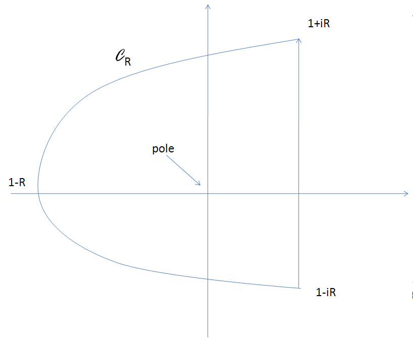
Figure 2. Contour of integration ${\mathcal{C}}_{R}$ for the integral in (3.18).

∎

It suffices to consider the case $m^{\prime}=m+1$ for all values of $m$ above a fixed threshold. In fact, given this particular case, the general statement can be derived with an iterative argument. To this end, we introduce a renormalization group transformation based on the notion of decorating path.

Definition 1.

(Decorating Paths.) Let $m\geq m_{0}$ and let $\gamma=\{y_{0},y_{1},y_{2},....\}$ be a symbolic sequence in $\Gamma_{m}$. A decorating path around $\gamma$ is defined as a symbolic sequence $\gamma^{\prime}=\{y_{0},y_{1}^{\prime},y_{2}^{\prime},....\}$ with $y_{i}^{\prime}\in h_{m+1}{\mathbb{Z}}$ containing the sequence $\gamma$ as a subset and such that if $y_{j}^{\prime}=y_{i}$ and $y_{k}^{\prime}=y_{i+1}$, then all elements $y_{n}^{\prime}$ with $j<n<k$ are such that $\lvert y_{n}^{\prime}-y_{j}^{\prime}\lvert\leq h_{m+1}$. Let ${\mathcal{D}}_{m+1}(\gamma)$ be the set of all decorating sequences around $\gamma$. The decorated weights are defined as follows:

(3.21) $${\tilde{W}}_{m}(\gamma,q;t)=\sum_{q^{\prime}=q}^{\infty}\sum_{\begin{matrix}\gamma^{\prime}\in{\mathcal{D}}_{m+1}(\gamma)\\ \gamma^{\prime}_{q^{\prime}}=\gamma_{q}\end{matrix}}W_{m+1}(\gamma^{\prime},q^{\prime};t).$$

Finally, let us introduce also the following Fourier transform:

(3.22) $$\hat{W}_{m}(\gamma,q;\omega)=\int_{0}^{\infty}W_{m}(\gamma,q;0,t)e^{i\omega t}dt,\;\;\;\;\hat{\tilde{W}}_{m}(\gamma,q;\omega)=\int_{0}^{\infty}\tilde{W}_{m}(\gamma,q;t)e^{i\omega t}dt.$$

Definition 2.

(Notations.) In the following, we set $h=h_{m+1}$ so that $h_{m}=2h$. We also use the Landau notation $O(h^{n})$ to indicate a function $f(h)$ such that $h^{-n}f(h)$ is bounded in a neighborhood of $(0)$.

Lemma 3.

Let $x,y\in A_{m}$ and let ${\mathcal{C}_{-}}$ be an integration contour as in Fig. 1. Then

(3.23) $$\bigg{\lvert}\bigg{(}\int_{{\mathcal{C}}_{-}}2G_{m+1}(x,y;\omega)-G_{m}(x,y;\omega)\bigg{)}e^{i\omega t}{d\omega\over 2\pi}\bigg{\lvert}=O(h^{2}).$$

Proof.

We have that

(3.24) $$2G_{m+1}(x,y;\omega)-G_{m}(x,y;\omega)= {1\over h}\sum_{q=1}^{\infty}2^{-q}\sum_{\begin{matrix}\gamma\in\Gamma_{m}:\gamma_{0}=x,\gamma_{q}=y\\ \lvert\gamma_{j}-\gamma_{j-1}\lvert=1\forall j\geq 1\end{matrix}}\left(2\hat{\tilde{W}}_{m}(\gamma,q;\omega)-\hat{W}_{m}(\gamma,q;\omega)\right).$$

The number of paths over which the summation is extended is

(3.25) $$N(\gamma,q;x,y)\equiv\sharp\{\gamma\in\Gamma_{m}:\gamma_{0}=x,\gamma_{q}=y,\lvert\gamma_{j}-\gamma_{j-1}\lvert=1\forall j\geq 1\}=\left(\begin{matrix}q\\ {q\over 2}+k\end{matrix}\right)$$

where $k={\lvert y-x\lvert\over h_{m}}.$ Applying Stirling’s formula we find

(3.26) $$N_{\gamma}\lesssim 2^{q}\sqrt{2\over\pi q}.$$

Hence

$$\bigg{\lvert}\int_{{\mathcal{C}}_{-}}\bigg{(}2G_{m+1}(x,y;\omega)-G_{m}(x,y;\omega)\bigg{)}e^{i\omega t}{d\omega\over 2\pi}\bigg{\lvert}$$

$$\leq{c\over h}\sum_{q=1}^{\infty}\sqrt{1\over q}\max_{\begin{matrix}\gamma\in\Gamma_{m}:\gamma_{0}=x,\gamma_{q}=y\\ \lvert\gamma_{j}-\gamma_{j-1}\lvert=1\forall j\geq 1\end{matrix}}\bigg{\lvert}\int_{{\mathcal{C}}_{-}}\bigg{(}2\hat{\tilde{W}}_{m}(\gamma,q;\omega)-\hat{W}_{m}(\gamma,q;\omega)\bigg{)}e^{i\omega t}{d\omega\over 2\pi}\bigg{\lvert}.$$

for some constant $c\approx\sqrt{2\over\pi}>0$. It suffices to extend the summation over $q$ only up to

(3.28) $$q_{\rm max}\equiv{e^{2}\Sigma_{1}^{2}t\over 2h^{2}}.$$

To resum beyond this threshold, one can use the previous lemma. More precisely, we have that

$$\bigg{\lvert}\int_{{\mathcal{C}}_{-}}\bigg{(}2G_{m+1}(x,y;\omega)-G_{m}(x,y;\omega)\bigg{)}e^{i\omega t}{d\omega\over 2\pi}\bigg{\lvert}$$

$$\leq{c\sqrt{q_{\rm max}}\over h}\max_{\begin{matrix}q,\gamma\in\Gamma_{m}:\gamma_{0}=x,\gamma_{q}=y\\ \lvert\gamma_{j}-\gamma_{j-1}\lvert=1\forall j\geq 1\end{matrix}}\bigg{\lvert}\int_{{\mathcal{C}}_{-}}\bigg{(}2\hat{\tilde{W}}_{m}(\gamma,q;\omega)-\hat{W}_{m}(\gamma,q;\omega)\bigg{)}e^{i\omega t}{d\omega\over 2\pi}\bigg{\lvert}.$$

Let $v(x)=\sigma(x)^{2}$. To evaluate the resummed weight function, let us form the matrix

(3.30) $$\bar{\mathcal{L}}(x;h)=\left(\begin{matrix}-{v\left(x+h\right)\over h^{2}}&&{v\left(x+h\right)\over 2h^{2}}-{\mu(x+h)\over 2h}&&0\\ {v\left(x\right)\over 2h^{2}}+{\mu(x)\over 2h}&&-{v\left(x\right)\over h^{2}}&&{v\left(x\right)\over 2h^{2}}-{\mu(x)\over 2h}\\ 0&&{v\left(x-h\right)\over 2h^{2}}+{\mu(x-h)\over 2h}&&-{v\left(x-h\right)\over h^{2}}\end{matrix}\right)$$

and decompose it as follows:

(3.31) $$\bar{\mathcal{L}}(x;h)={1\over h^{2}}\bar{\mathcal{L}}_{0}(x)+{1\over h}\bar{\mathcal{L}}_{1}(x)+\bar{\mathcal{L}}_{2}(x)+h\bar{\mathcal{L}}_{3}(x)+O(h^{2}).$$

where

(3.32) $$\bar{\mathcal{L}}_{0}(x)=\left(\begin{matrix}-v(x)&&{1\over 2}{v(x)}&&0\\ {1\over 2}{v(x)}&&-{v(x)}&&{1\over 2}{v(x)}\\ 0&&{1\over 2}{v(x)}&&-{v(x)}\end{matrix}\right),$$

(3.33) $$\bar{\mathcal{L}}_{1}(x)=\left(\begin{matrix}-v^{\prime}(x)&&{1\over 2}v^{\prime}(x)-{1\over 2}\mu(x)&&0\\ {1\over 2}\mu(x)&&0&&-{1\over 2}\mu(x)\\ 0&&-{1\over 2}v^{\prime}(x)+{1\over 2}\mu(x)&&v^{\prime}(x)\end{matrix}\right),$$

(3.34) $$\bar{\mathcal{L}}_{2}(x)=\left(\begin{matrix}-{1\over 2}v^{\prime\prime}(x)&&{1\over 4}v^{\prime\prime}(x)-{1\over 2}\mu^{\prime}(x)&&0\\ 0&&0&&0\\ 0&&{1\over 4}v^{\prime\prime}(x)-{1\over 2}\mu^{\prime}(x)&&-{1\over 2}v^{\prime\prime}(x)\end{matrix}\right).$$

and

(3.35) $$\bar{\mathcal{L}}_{3}(x)=\left(\begin{matrix}-{1\over 6}v^{\prime\prime\prime}(x)&&{1\over 12}v^{\prime\prime\prime}(x)-{1\over 4}\mu^{\prime\prime}(x)&&0\\ 0&&0&&0\\ 0&&-{1\over 12}v^{\prime\prime\prime}(x)+{1\over 4}\mu^{\prime\prime}(x)&&{1\over 6}v^{\prime\prime\prime}(x)\end{matrix}\right).$$

Let us introduce the sign variable $\tau=\pm 1$, the functions

(3.36) $$\phi_{0}(t,x,\tau) \equiv 2{\mathcal{L}}_{m}(x,x+2\tau h)e^{t{\mathcal{L}}_{m}(x,x)}1(t\geq 0)$$

(3.37) $$\phi_{1}(t,x,\tau) \equiv 2{\mathcal{L}}_{m+1}(x+\tau h,x+2\tau h)e^{t\bar{\mathcal{L}}(x;h)}(x,x+\tau h)1(t\geq 0)$$

and their Fourier transforms

$$\hat{\phi}_{0}(\omega,x,\tau) =\left({v(x)\over 4h^{2}}+\tau{\mu(x)\over 2h}\right)\left({v(x)\over 4h^{2}}+i\omega\right)^{-1}$$

$$\hat{\phi}_{1}(\omega,x,\tau) =\left({v(x)\over h^{2}}+\tau{\mu(x)+v^{\prime}(x)\over h}+{v^{\prime\prime}(x)+\mu^{\prime}(x)\over 2}+\left({v^{\prime\prime\prime}(x)\over 6}+{\mu^{\prime\prime}(x)\over 2}\right)\tau h+O(h^{2})\right)$$

(3.38) $$\hskip 227.62204pt<x\lvert\left(-\bar{\mathcal{L}}(x;h)+i\omega\right)^{-1}\lvert x+\tau h>.$$

where

(3.39) $$\lvert x>=\left(\begin{matrix}0\\ 1\\ 0\end{matrix}\right),\;\;\;\;{\rm and}\;\;\;\;\lvert x+\tau h>=\left(\begin{matrix}\delta_{\tau,1}\\ 0\\ \delta_{\tau,-1}\end{matrix}\right).$$

We also require the functions

(3.40) $$\psi_{0}(t,x)\equiv e^{t{\mathcal{L}}_{m}(x,x)}1(t\geq 0),\;\;\;\;\;\;\psi_{1}(t,x)\equiv e^{t\bar{\mathcal{L}}(y;h)}(x,x)1(t\geq 0)$$

and the corresponding Fourier transforms

(3.41) $$\hat{\psi}_{0}(\omega,x)=\left({v(x)\over 4h^{2}}+i\omega\right)^{-1},\;\;\;\;\;\hat{\psi}_{1}(\omega,x)=<x\lvert\left(-\bar{\mathcal{L}}(x;h)+i\omega\right)^{-1}\lvert x>.$$

If $\gamma$ is a symbolic sequence, then

(3.42) $$\hat{W}_{m}(\gamma,q;\omega) =\hat{\psi}_{0}(\omega,\gamma_{q})\prod_{j=0}^{q-1}\hat{\phi}_{0}(\omega;\gamma_{j},{\rm sgn}(\gamma_{j+1}-\gamma_{j}))$$

(3.43) $$\hat{\tilde{W}}_{m}(\gamma,q;\omega) =\hat{\psi}_{1}(\omega,\gamma_{q})\prod_{j=0}^{q-1}\hat{\phi}_{1}(\omega;\gamma_{j},{\rm sgn}(\gamma_{j+1}-\gamma_{j})).$$

Let us estimate the difference between the functions $\hat{\phi}_{1}(\omega,x,\tau)$ and $\hat{\phi}_{2}(\omega,x,\tau)$ assuming that $\omega$ is in the contour ${\mathcal{C}}_{-}$ in Fig. 2. Retaining only terms up to order up to $O(h^{3})$, we find

$$\hat{\phi}_{0}(\omega,x,\tau)=1+{2\mu(x)\tau h\over v(x)}-{4i\omega h^{2}\over v(x)}-8\mu(x){i\omega\tau h^{3}\over v(x)^{2}}-{16\omega^{2}h^{4}\over v(x)^{2}}+O(h^{5}).$$

A lengthy but straightforward calculation which is best carried out using a symbolic manipulation program, gives

$$\hat{\phi}_{1}(\omega,x,\tau)=1+{2\mu(x)\tau h\over v(x)}-{4i\omega h^{2}\over v(x)}-\big{[}8\mu(x)-v^{\prime}(x)\big{]}{i\omega\tau h^{3}\over v(x)^{2}}$$

$$\hskip 170.71652pt+r(x)\cdot h^{3}\tau+i\omega h^{4}p(x)-{14\omega^{2}h^{4}\over v(x)^{2}}+O(h^{5})$$

where

$$r(x)={1\over 2v(x)^{3}}\big{[}\mu^{\prime\prime}(x)v(x)-4\mu(x)^{3}+2v^{\prime}(x)\mu(x)^{2}-2v^{\prime}(x)v(x)\mu^{\prime}(x)$$

$$\hskip 170.71652pt-\big{(}2\mu(x)\mu^{\prime}(x)+v^{\prime\prime}(x)v(x)-2v^{\prime}(x)^{2}\big{)}\mu(x)\big{]}.$$

$$p(x)={1\over v(x)^{3}}\big{[}4\mu(x)^{2}-2v^{\prime}(x)\mu(x)+4v(x)\mu^{\prime}(x)+v^{\prime\prime}(x)v(x)-2v^{\prime}(x)^{2}\big{]}.$$

We have that

$$\sum_{j=0}^{q-1}\bigg{(}\log\hat{\phi}_{0}(\omega;\gamma_{j},{\rm sgn}(\gamma_{j+1}-\gamma_{j}))-\log\hat{\phi}_{1}(\omega;\gamma_{j},{\rm sgn}(\gamma_{j+1}-\gamma_{j}))\bigg{)}$$

$$=\sum_{j=0}^{q-1}\bigg{(}{i\omega v^{\prime}(\gamma_{j})\over v(\gamma_{j})^{2}}+r(\gamma_{j})\bigg{)}h^{3}{\rm sgn}(\gamma_{j+1}-\gamma_{j})+\big{(}\lvert\omega\lvert\lvert\lvert p\lvert\lvert_{\infty}+2\lvert\omega\lvert^{2}\lvert\lvert v^{-2}\lvert\lvert_{\infty}\big{)}O(h^{4}q)$$

$$=i\omega h^{2}\log\bigg{(}{v(\gamma_{q})\over v(\gamma_{0})}\bigg{)}+h^{2}\big{(}R(\gamma_{q})-R(\gamma_{0})\big{)}+\big{(}\lvert\omega\lvert\lvert\lvert p\lvert\lvert_{\infty}+2\lvert\omega\lvert^{2}\lvert\lvert v^{-2}\lvert\lvert_{\infty}\big{)}O(h^{4}q)$$

where $R(x)$ is a primitive of $r(x)$, i.e.

(3.48) $$R(x)=\int^{x}r(z)dz.$$

We conclude that there is a constant $c>0$ such that

(3.49) $$\bigg{\lvert}\int_{{\mathcal{C}}_{-}}\bigg{(}\prod_{j=0}^{q-1}\hat{\phi}_{0}(\omega;\gamma_{j},{\rm sgn}(\gamma_{j+1}-\gamma_{j}))-\prod_{j=0}^{q-1}\hat{\phi}_{1}(\omega;\gamma_{j},{\rm sgn}(\gamma_{j+1}-\gamma_{j}))\bigg{)}e^{i\omega t}{d\omega\over 2\pi}\bigg{\lvert}\leq ch^{2}.$$

for all $q\leq q_{\max}$. Here we use the decay of $e^{i\omega t}$ in the upper half of the complex $\omega$ plane to offset the $\omega$ dependencies in the integrand. Similar calculations lead to the following expansions:

(3.50) $$\hat{\psi}_{0}(\omega,y)={4h^{2}\over v(y)}+O(\omega h^{4}),\;\;\;\;\;\hat{\psi}_{1}(\omega,y)={2h^{2}\over v(y)}+O(\omega h^{4})={1\over 2}\hat{\psi}_{0}(\omega,y)+O(\omega h^{4}).$$

Since $q<ch^{-2}$ and $\omega\leq\lvert\log h\lvert$, we find

(3.51) $$\bigg{\lvert}\int_{{\mathcal{C}}_{-}}\bigg{(}2G_{m+1}(x,y;\omega)-G_{m}(x,y;\omega)\bigg{)}e^{i\omega t}{d\omega\over 2\pi}\bigg{\lvert}\leq c{\sqrt{q_{\rm max}}\over h}h^{4}\leq ch^{2}.$$

This completes the proof of the Lemma and of the Theorem. ∎

By differentiating with respect to time in equation 3.52, we find that

(3.52) $${\partial\over\partial t}u_{m}(x,y;t)=\int_{{\mathcal{C}}_{-}}{d\omega\over 2\pi}i\omega G_{m}(x,y;\omega)e^{i\omega t}+\int_{{\mathcal{C}}_{+}}{d\omega\over 2\pi}i\omega G_{m}(x,y;\omega)e^{i\omega t}.$$

All the derivations above carry through and we conclude that

(3.53) $$\bigg{\lvert}\int_{{\mathcal{C}}_{+}}{d\omega\over 2\pi}i\omega G_{m}(x,y;\omega)e^{i\omega t}\bigg{\lvert}\leq ch^{2}.$$

and also

(3.54) $$\bigg{\lvert}\int_{{\mathcal{C}}_{-}}i\omega\bigg{(}2G_{m+1}(x,y;\omega)-G_{m}(x,y;\omega)\bigg{)}e^{i\omega t}{d\omega\over 2\pi}\bigg{\lvert}\leq c{\sqrt{q_{\rm max}}\over h}h^{4}\leq ch^{2}.$$

Hence the first time derivatives of the kernel satisfy the same Cauchy convergence condition as the kernel itself.

4. Lesser Smooth Coefficients

In this section we assume coefficients are either Hölder continuous or obey the conditions in Theorem 2.

Lemma 4.

Let $f(x)$ be a continuous function in $[-L,L]$ satisfying periodic boundary conditions. Then, for all $h>0$, we have that

(4.1) $$f(x+h_{m})=f(x)+h_{m}\nabla^{m}_{x}f(x)+{h^{2}\over 2}\Delta^{m}_{x}f(x)$$

(4.2) $$f(x-h_{m})=f(x)-h_{m}\nabla^{m}_{x}f(x)+{h^{2}\over 2}\Delta^{m}_{x}f(x).$$

This is the result of a simple calculation, which is however useful as it allows one to extend the derivation in the previous section by making the following replacements:

(4.3) $$v^{\prime}(x)\to\nabla^{m}_{x}v(x),\;\;\;\;v^{\prime\prime}(x)\to\Delta^{m}v(x),\;\;\;\;v^{\prime\prime\prime}(x)\to 0$$

(4.4) $$\mu^{\prime}(x)\to\nabla^{m}_{x}\mu(x),\;\;\;\;\mu^{\prime\prime}(x)\to\Delta^{m}_{x}\mu(x).$$

In fact,

(4.5) $$\bar{\mathcal{L}}(x;h)={1\over h^{2}}\bar{\mathcal{L}}_{0}(x)+{1\over h}\bar{\mathcal{L}}_{1}(x)+\bar{\mathcal{L}}_{2}(x)+h\bar{\mathcal{L}}_{3}(x)$$

without any $O(h^{3})$ corrections as long as one re-defines the matrices on the right hand side as follows:

(4.6) $$\bar{\mathcal{L}}_{0}(x)=\left(\begin{matrix}-v(x)&&{1\over 2}{v(x)}&&0\\ {1\over 2}{v(x)}&&-{v(x)}&&{1\over 2}{v(x)}\\ 0&&{1\over 2}{v(x)}&&-{v(x)}\end{matrix}\right),$$

(4.7) $$\bar{\mathcal{L}}_{1}(x)=\left(\begin{matrix}-\nabla_{x}^{m}v(x)&&{1\over 2}\nabla_{x}^{m}v(x)-{1\over 2}\mu(x)&&0\\ {1\over 2}\mu(x)&&0&&-{1\over 2}\mu(x)\\ 0&&-{1\over 2}\nabla_{x}^{m}v(x)+{1\over 2}\mu(x)&&\nabla_{x}^{m}v(x)\end{matrix}\right),$$

(4.8) $$\bar{\mathcal{L}}_{2}(x)=\left(\begin{matrix}-{1\over 2}\Delta_{x}^{m}v(x)&&{1\over 4}\Delta_{x}^{m}v(x)-{1\over 2}\nabla_{x}^{m}\mu(x)&&0\\ 0&&0&&0\\ 0&&{1\over 4}\Delta_{x}^{m}v(x)-{1\over 2}\nabla_{x}^{m}\mu(x)&&-{1\over 2}\Delta_{x}^{m}v(x)\end{matrix}\right).$$

and

(4.9) $$\bar{\mathcal{L}}_{3}(x)=\left(\begin{matrix}0&&-{1\over 4}\Delta_{x}^{m}\mu(x)&&0\\ 0&&0&&0\\ 0&&{1\over 4}\Delta_{x}^{m}\mu(x)&&0\end{matrix}\right).$$

All derivations in the previous section go through formally unchanged and one arrives at the following expressions

$$\hat{\phi}_{0}(\omega,x,\tau)=1+{2\mu(x)\tau h\over v(x)}-{4i\omega h^{2}\over v(x)}-8\mu(x){i\omega\tau h^{3}\over v(x)^{2}}-{16\omega^{2}h^{4}\over v(x)^{2}}+O(h^{5}).$$

and

$$\hat{\phi}_{1}(\omega,x,\tau)=1+{2\mu(x)\tau h\over v(x)}-{4i\omega h^{2}\over v(x)}-\big{[}8\mu(x)-\nabla^{m}_{x}v(x)\big{]}{i\omega\tau h^{3}\over v(x)^{2}}$$

$$\hskip 170.71652pt+r(x)\cdot h^{3}\tau+i\omega h^{4}p(x)-{14\omega^{2}h^{4}\over v(x)^{2}}+O(h^{5})$$

where

$$r(x)={1\over 2v(x)^{3}}\big{[}\Delta^{m}_{x}\mu(x)v(x)-4\mu(x)^{3}+2\nabla^{m}_{x}v(x)\mu(x)^{2}-2\nabla^{m}_{x}v(x)v(x)\nabla^{m}_{x}\mu(x)$$

$$\hskip 170.71652pt-\big{(}2\mu(x)\nabla^{m}_{x}\mu(x)+\Delta^{m}_{x}v(x)v(x)-2\nabla^{m}_{x}v(x)^{2}\big{)}\mu(x)\big{]}.$$

$$p(x)={1\over v(x)^{3}}\big{[}4\mu(x)^{2}-2\nabla^{m}_{x}v(x)\mu(x)+4v(x)\nabla^{m}_{x}\mu(x)+\Delta^{m}_{x}v(x)v(x)-2\nabla^{m}_{x}v(x)^{2}\big{]}.$$

We have that

$$\bigg{\lvert}\sum_{j=0}^{q-1}\bigg{(}\log\hat{\phi}_{0}(\omega;\gamma_{j},{\rm sgn}(\gamma_{j+1}-\gamma_{j}))-\log\hat{\phi}_{1}(\omega;\gamma_{j},{\rm sgn}(\gamma_{j+1}-\gamma_{j}))\bigg{)}\bigg{\lvert}$$

$$\leq\bigg{\lvert}\sum_{j=0}^{q-1}\bigg{(}{i\omega\nabla^{m}_{\gamma_{j}}v(\gamma_{j})\over v(\gamma_{j})^{2}}+r(\gamma_{j})\bigg{)}h^{3}{\rm sgn}(\gamma_{j+1}-\gamma_{j})\bigg{\lvert}+\big{(}\lvert\omega\lvert\lvert\lvert p\lvert\lvert_{\infty}+2\lvert\omega\lvert^{2}\lvert\lvert v^{-2}\lvert\lvert_{\infty}\big{)}O(h^{4}q).$$

$$\leq 2Lh^{2}\sup_{x\in A_{m}}\bigg{\lvert}{i\omega\nabla^{m}_{x}v(x)\over v(x)^{2}}+r(x)\bigg{\lvert}+\big{(}\lvert\omega\lvert\lvert\lvert p\lvert\lvert_{\infty}+2\lvert\omega\lvert^{2}\lvert\lvert v^{-2}\lvert\lvert_{\infty}\big{)}O(h^{4}q)\leq ch^{\gamma}.$$

where in the last step we made use of the Hölder continuity assumptions of Theorem 1. The other bounds staying the same, we arrive at

(4.14) $$\bigg{\lvert}\int_{{\mathcal{C}}_{-}}\bigg{(}2G_{m+1}(x,y;\omega)-G_{m}(x,y;\omega)\bigg{)}e^{i\omega t}{d\omega\over 2\pi}\bigg{\lvert}\leq c{\sqrt{q_{\rm max}}\over h}h^{2+\gamma}\leq ch^{\gamma}.$$

Under the weaker assumption of Theorem 2, the bound that applies is instead

(4.15) $$\bigg{\lvert}\int_{{\mathcal{C}}_{-}}\bigg{(}2G_{m+1}(x,y;\omega)-G_{m}(x,y;\omega)\bigg{)}e^{i\omega t}{d\omega\over 2\pi}\bigg{\lvert}\leq c{\sqrt{q_{\rm max}}\over h}h^{2}\rho(h)\leq c\rho(h).$$

Similar bounds also extend to the case of the first time derivative, since multiplication by a factor $i\omega$ inside of the contour integral is immaterial as far as establishing a bound of this sort is concerned. This completes the proof of Theorem 1 and Theorem 2.

5. Explicit Euler Scheme

In this section we prove Theorem 3. A Dyson expansion can also be obtained for the time-discretized kernel and has the form

$$u_{m}^{\delta t}(y_{1},y_{2};t)= {1\over h_{m}}\sum_{q=1}^{\infty}\sum_{\gamma\in\Gamma_{m}:\gamma_{0}=x,\gamma_{q}=y}\sum_{k_{1}=1}^{N}\sum_{k_{2}=k_{1}+1}^{N}...\sum_{k_{q}=k_{q-1}+1}^{N}$$

(5.1) $$\bigg{(}1+\delta t{\mathcal{L}}_{m}(\gamma_{0},\gamma_{0})\bigg{)}^{k_{1}-1}(\delta t)^{q}\prod_{j=1}^{q}{\mathcal{L}}_{m}(\gamma_{j-1},\gamma_{j})\bigg{(}1+\delta t{\mathcal{L}}_{m}(\gamma_{j},\gamma_{j})\bigg{)}^{k_{j+1}-k_{j}-1}$$

where $t_{q+1}=t$ and $k_{q+1}=N$. In this case, the propagator can be expressed through a Fourier integral as follows:

(5.2) $$u_{m}^{\delta t}(y_{1},y_{2};t)=\int_{-{\pi\over\delta t}}^{\pi\over\delta t}G_{m}^{\delta t}(y_{1},y_{2};\omega)e^{i\omega t}{d\omega\over 2\pi}$$

where

(5.3) $$G_{m}^{\delta t}(y_{1},y_{2};\omega)=\delta t\sum_{j=0}^{t\over\delta t}u_{m}^{\delta t}(y_{1},y_{2};j\delta t)e^{-i\omega j\delta t}.$$

The propagator can also be represented as the limit

(5.4) $$u_{m}^{\delta t}(y_{1},y_{2};t)=\lim_{H\to\infty}\int_{{\mathcal{C}}_{H}}G_{m}^{\delta t}(y_{1},y_{2};\omega)e^{i\omega t}{d\omega\over 2\pi}$$

where ${\mathcal{C}}_{H}$ is the contour in Fig. 3. This is due to the fact that the integral along the segments $BC$ and $DA$ are the negative of each other, while the integral over $CD$ tends to zero exponentially fast as $\Im(\omega)\to\infty$, where $\Im(\omega)$ is the imaginary part of $\omega$. Using Cauchy’s theorem, the contour in Fig. 3 can be deformed into the contour in Fig. 1. To estimate the discrepancy between the time-discretized kernel and the continuous time one, one can thus compare the Green’s function along such contour. Again, the only arc that requires detailed attention is the arc $BCD$, as the integral over rest of the contour of integration can be bounded from above as in the previous section.

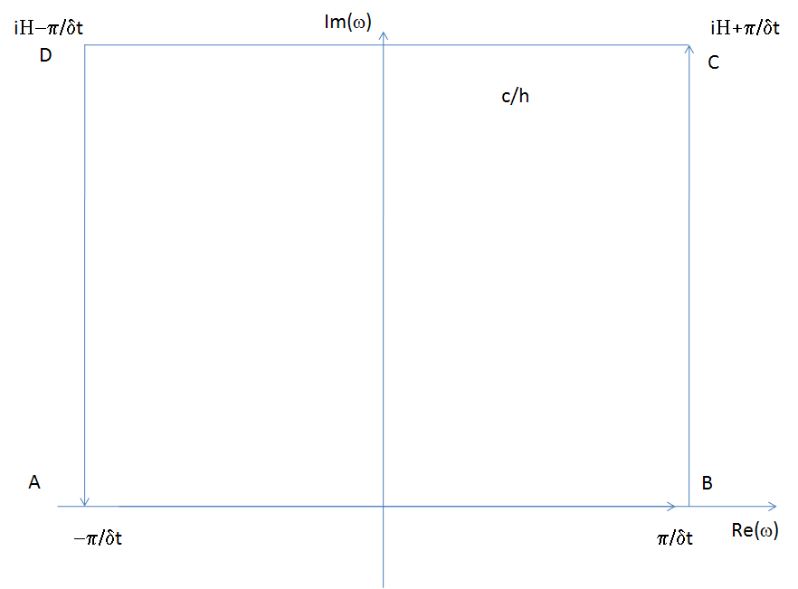
Figure 3. Contour of integration for the integral in (5.4).

Let $h=h_{m}$ and let us introduce the two functions

(5.5) $$\phi_{0}(t,x,\tau) \equiv 2{\mathcal{L}}_{m}(x,x+\tau h)e^{t{\mathcal{L}}_{m}(x,x)}1(t\geq 0),$$

(5.6) $$\phi_{\delta t}(j,x,\tau) \equiv 2{\mathcal{L}}_{m}(x,x+\tau h)\big{(}1+\delta t{\mathcal{L}}_{m}(x,x)\big{)}^{j-1}.$$

and the corresponding Fourier transforms

(5.7) $$\hat{\phi}_{0}(\omega,x,\tau) =\int_{0}^{\infty}\phi_{0}(t,x,\tau)e^{-i\omega t}{d\omega\over 2\pi}=\left({v(x)\over h^{2}}+\tau{\mu(x)\over h}\right)\left({v(x)\over h^{2}}+i\omega\right)^{-1}$$

(5.8) $$\hat{\phi}_{\delta t}(\omega,x,\tau) =\sum_{j=0}^{t\over\delta t}\phi_{\delta t}(j,x,\tau)e^{-i\omega j\delta t}=\left({v(x)\over h^{2}}+\tau{\mu(x)\over h}\right)\left(e^{i\omega\delta t}-1+\delta t{v(x)\over h^{2}}\right)^{-1}.$$

We have that

$$\hat{\phi}_{\delta t}(\omega,x,\tau) =\left({v(x)\over h^{2}}+\tau{\mu(x)\over h}\right)\left(i\omega+{v(x)\over h^{2}}-{\omega^{2}\over 2}\delta t+O(\delta t^{2})\right)^{-1}$$

(5.9) $$=\hat{\phi}_{0}(\omega,x,\tau)+{\omega^{2}\over 2v(x)}h^{2}\delta t+O(h^{2}\delta t^{2}).=\hat{\phi}_{0}(\omega,x,\tau)+O(h^{4}),$$

where the last step uses the fact that $\delta t=O(h^{2})$.

Let us also introduce the functions

(5.10) $$\psi_{0}(t,x,\tau) \equiv e^{t{\mathcal{L}}_{m}(x,x)}1(t\geq 0),\hskip 28.45274pt\psi_{\delta t}(j,x,\tau)\equiv\sum_{k=1}^{j}\big{(}1+\delta t{\mathcal{L}}_{m}(x,x)\big{)}^{j-1}.$$

and the corresponding Fourier transforms

(5.11) $$\hat{\psi}_{0}(\omega,x,\tau) =\left({v(x)\over h^{2}}+i\omega\right)^{-1},\hskip 28.45274pt\hat{\psi}_{\delta t}(\omega,x,\tau)=\left(e^{i\omega\delta t}-1+\delta t{v(x)\over h^{2}}\right)^{-1}.$$

Again we find that

(5.12) $$\hat{\psi}_{0}(\omega,x,\tau)=\hat{\psi}_{\delta t}(\omega,x,\tau)+O(h^{4}).$$

If $\gamma$ is a symbolic sequence, then let us set

(5.13) $$\hat{W}_{m}(\gamma,q;\omega) =\hat{\psi}_{0}(\omega,\gamma_{q})\prod_{j=0}^{q-1}\hat{\phi}_{0}(\omega;\gamma_{j},{\rm sgn}(\gamma_{j+1}-\gamma_{j}))$$

(5.14) $$\hat{W}_{m}^{\delta t}(\gamma,q;\omega) =\hat{\psi}_{\delta t}(\omega,\gamma_{q})\prod_{j=0}^{q-1}\hat{\phi}_{\delta t}(\omega;\gamma_{j},{\rm sgn}(\gamma_{j+1}-\gamma_{j})).$$

We have that

(5.15) $$G^{\delta t}_{m}(x,y;\omega)-G_{m}(x,y;\omega)= {1\over h}\sum_{q=1}^{\infty}2^{-q}\sum_{\begin{matrix}\gamma\in\Gamma_{m}:\gamma_{0}=x,\gamma_{q}=y\\ \lvert\gamma_{j}-\gamma_{j-1}\lvert=1\forall j\geq 1\end{matrix}}\left(\hat{W}_{m}^{\delta t}(\gamma,q;\omega)-\hat{W}_{m}(\gamma,q;\omega)\right).$$

The integration over the contour in Fig. 1 can again be split into an integration over the countour ${\mathcal{C}}_{-}$ and an integration over ${\mathcal{C}}_{+}$. The integral over ${\mathcal{C}}_{+}$ can be bounded from above thanks to Lemma 1. Furthermore, we have that

$$\bigg{\lvert}\int_{{\mathcal{C}}_{-}}\bigg{(}G^{\delta t}_{m}(x,y;\omega)-G_{m}(x,y;\omega)\bigg{)}e^{i\omega t}{d\omega\over 2\pi}\bigg{\lvert}$$

$$\leq ch^{-1}\sqrt{q_{\rm max}}\max_{\begin{matrix}q,\gamma\in\Gamma_{m}:\gamma_{0}=x,\gamma_{q}=y\\ \lvert\gamma_{j}-\gamma_{j-1}\lvert=1\forall j\geq 1\end{matrix}}\bigg{\lvert}\int_{{\mathcal{C}}_{-}}\bigg{(}\hat{W}_{m}^{\delta t}(\gamma,q;\omega)-\hat{W}_{m}(\gamma,q;\omega)\bigg{)}e^{i\omega t}{d\omega\over 2\pi}\bigg{\lvert}.$$

(5.16) $$\leq ch^{2}$$

To bound the time derivative, we have to consider

$$\bigg{\lvert}\int_{{\mathcal{C}}_{-}}\bigg{(}{e^{i\omega\delta t}-1\over\delta t}G^{\delta t}_{m}(x,y;\omega)-i\omega G_{m}(x,y;\omega)\bigg{)}e^{i\omega t}{d\omega\over 2\pi}\bigg{\lvert}$$

But, since $\delta t=O(h^{2})$, also this difference is $O(h^{2})$.

6. Conclusions

We obtained bounds on convergence rates for explicit discretization schemes to the kernel of one-dimensional diffusion equations with continuous coefficients. We consider both semidiscrete triangulations with continuous time and explicit Euler schemes with time step small enough for the method to be stable. The proof is constructive and based on a new technique of path conditioning for Markov chains and a renormalization group argument. Convergence rates depend on the degree of smoothness and Hölder differentiability of the coefficients. The method is of more general applicability and will be extended in future work.

References

[1]\harvarditem[Albanese and Mijatovic]Albanese and
Mijatovic2006AlbaneseMijatovicBM
Albanese, C. and A. Mijatovic (2006). Convergence Rates for Diffusions on
Continuous-Time Lattices. preprint, available at
www.level3finance.com.
[2]\harvarditem[Baker et al.]Baker et al.1977BakerBrambleThomte
Baker, G., J. Bramble and V. Thomee (1977). Single Step Galerkin
Approximations for Parabolic Problems. Math. Comp.31, 818–847.
[3]\harvarditem[Ethier and Kurtz]Ethier and Kurtz1986EthierKurtz
Ethier, S.N. and T.G. Kurtz (1986). Markov processes: Characterization
and convergence. John Wiley and Sons, New York.
[4]\harvarditem[Fabes and Riviere]Fabes and Riviere1966FabesRiviere
Fabes, E. B. and N. M. Riviere (1966). Parabolic Partial Differential
Equations with Uniformly Continuous Coefficients. Bull. Amer.
Math. Soc.72, 116–117.
[5]\harvarditem[Feller]Feller1936Feller1936
Feller, W. (1936). Zur theorie der stochastischen prozesse [existenz und
eindeutigkeitssatze]. Math. Ann.113, 113–160.
[6]\harvarditem[Feller]Feller1952Feller52
Feller, W. (1952). The parabolic differential equations and tke associated
semi-groups of transformutions. Ann. of Math.55, 468–519.
[7]\harvarditem[Friedrichs]Friedrichs1958Friedrichs
Friedrichs, K. O. (1958). Symmetric positive linear differential equations.
Cornm. Pure Appl. Math.11, 333–418.
[8]\harvarditem[Hille]Hille1948Hille
Hille, E. (1948). Functional analysis and semi-groups. Amer. Math. Soc.
Colloquium Publications.
[9]\harvarditem[Ito]Ito1957Ito57
Ito, K. (1957). Fundamental solutions of parabolic differential equations and
boundary value problems. Jap. J. Math.27, 55–102.
[10]\harvarditem[Kato]Kato1966Kato
Kato, T. (1966). perturbation Theory for Linear Operators. Springer, New
York.
[11]\harvarditem[Kolmogorov]Kolmogorov1931Kolmogorov1931
Kolmogorov, A. N. (1931). Uber die analytischen methoden in der
wahrscheinlichkeitsrechnung. Math. Ann.104, 415–458.
[12]\harvarditem[Kurtz]Kurtz1969Kurtz
Kurtz, T. (1969). Extensions of Trotter’s operator semigroup approximation
theorems. J. Funct. Anal.3, 354–375.
[13]\harvarditem[Lax and Phillips]Lax and Phillips1960LaxPhilips
Lax, P. D. and R. S. Phillips (1960). Local boundary conditions for
dissipative symmetric linear differential operators. Cornm. Pure Appl.
Math.13, 427–455.
[14]\harvarditem[Luskin and Rannacher]Luskin and Rannacher1978LuskinRannacher
Luskin, M. and R. Rannacher (1978). On the Smoothing Property of the
Galerkin Method for Parabolic Equations. Proc. Japan Acad. Ser.
A Math. Sci.54, 326–331.
[15]\harvarditem[Mingyou and Thomee]Mingyou and Thomee1982MingyouThomee
Mingyou, H. and V. Thomee (1982). On the Backward Euler Method for
Parabolic Equations with Rough Initial Data. SIAM J. Numer.
Anal19, 599–603.
[16]\harvarditem[Palencia]Palencia1996Palencia
Palencia, C. (1996). Maximum Norm Analysis of Completely Discrete
Finite Element Methods for Parabolic Problems. SIAM Journal on
Numerical Analysis33, 1654–1668.
[17]\harvarditem[Philips]Philips1961Philips
Philips, R. S. (1961). On the integration of the diffusion equation with
boundary conditions. Transactions of the American Mathematical Society98, 62–84.
[18]\harvarditem[Sova]Sova1967Sova
Sova, M. (1967). Convergence d’operations lineaires non bornees. Rev.
Roumaine Math. Pures Appliq.12, 373–389.
[19]\harvarditem[Stroock and Varadhan]Stroock and Varadhan1969SV1969
Stroock, D.W. and S.R.S. Varadhan (1969). Diffusion processes with continuous
coefficients, i and ii.. Comm. Pure Appl. Math.22, 345–400,
479–530.
[20]\harvarditem[Stroock and Varadhan]Stroock and Varadhan1979SV
Stroock, D.W. and S.R.S. Varadhan (1979). Multidimensional diffusion
processes. Springer-Verlag, Berlin.
[21]\harvarditem[Suzuki]Suzuki1978Suzuki
Suzuki, T. (1978). On the Rate of Convergence of the Difference Finite
Element Approximation for Parabolic Equations. Proc. Japan Acad.
Ser. A Math. Sci.54, 326–331.
[22]\harvarditem[Yosida]Yosida1951Yosida
Yosida, K. (1951). Integration of fokker-planck’s equation with a boundary
condition. J. Math. Soc. Japan3, 69–73.
[23]
Conversion to HTML had a Fatal error and exited abruptly. This document may be truncated or damaged.