Free Fermions and Thermal AdS/CFT

Abstract:

The dynamics of finite temperature $U(N)$ gauge theories on $S^{3}$ can be described, at weak coupling, by an effective unitary matrix model. Here we present an exact solution to these models, for any value of $N$, in terms of a sum over representations. Taking the large $N$ limit of this solution provides a new perspective on the deconfinement transition which is supposed to be dual to the Hawking-Page transition. The large $N$ phase transition manifests itself here in a manner similar to the Douglas-Kazakov phase transition in $2d$ Yang-Mills theory. We carry out a complete analysis of the saddle representation in the simplest case involving only the order parameter ${\rm Tr}U$. We find that the saddle points corresponding to thermal $AdS$, the small black hole and the large black hole can all be described in terms of free fermions. They all admit a simple phase space description a la the BPS geometries of Lin, Lunin and Maldacena.

1 Introduction

Though we know of many instances where a gauge theory is a holographic description of a gravitational theory, we are yet to understand the precise way in which a local diffeomorphism invariant theory in one higher dimension is encoded in the dynamics of the gauge theory. In a sense, the redundancy of diffeomorphisms has been largely eliminated in the gauge theory description. But this has come at the cost of losing information about the locality of the bulk description. Is there a natural way in the gauge theory to restore the redundancies which characterise the geometrical description of the bulk?

A partial hint comes from the beautiful work of Lin, Lunin and Maldacena [1] who showed that the geometry of a class of half-BPS solutions of the bulk theory is completely fixed by specifying a single function of two of the bulk coordinates. This function, which takes values either zero or one in the entire two dimensional plane, was identified with the phase space distribution of free fermions describing the half BPS dynamics in the gauge theory. In other words, the configuration space of the bulk, with its redundancies, was identified with the phase space of the boundary degrees of freedom. In fact, the quantisation of the space of BPS configurations on the gravity side agrees with those of the free fermions [2][3]. Notice that the fermionic phase space description is also a redundant one since it is the shape of the perimeter of the ”filled fermi” sea that completely determines everything. The phase space picture therefore appears to be a step in the right direction.

However, the half-BPS case seems to be very special and the picture of free fermions is not likely to be generally applicable. It is therefore a bit of a surprise that, in this paper, we find a similar free fermion phase space description in the non-supersymmetric context of finite temperature AdS/CFT. It is very well known [4] that the thermal partition function of the gauge theory exhibits a behaviour which is qualitatively similar to the Hawking-Page [5] phase diagram on the gravity side. In particular, we find a free fermionic description in the weakly coupled gauge theory, for each of the saddle points that correspond to Thermal AdS, the (unstable) ”small” AdS Schwarschild black hole as well as the ”big” AdS black hole. In each case there is a simple region in phase space which is the filled fermi sea.

Our starting point is the effective unitary matrix model that describes the holonomies of the Polyakov loop at weak gauge coupling [6][8]. As was argued in [8], in the free $U(N)$ Yang-Mills theory on $S^{3}$ at finite temperature, all modes are massive and can be exactly integrated out, except for the zero mode of $A_{0}$. The dynamics of this interacting mode is naturally expressed in terms of a unitary matrix model for the holonomy $U$, along the thermal $S^{1}$. At weak coupling, we can continue to integrate out all the other modes and end up with (a more complicated) effective matrix model for $U$. These matrix models have been well analysed, in the large $N$ limit, in terms of the collective field $\sigma(\theta)$ which is the eigenvalue density of $U$. They have been shown to exhibit a phase structure which describes the deconfinement transition and is qualitatively very similar to that of the Hawking-Page description of AdS gravity at finite temperature [8][9][10].

In this paper, we present an exact solution to the partition function of these matrix models, which is valid for any finite $N$. The answer is in terms of characters of the conjugacy classes of the symmetric group with a sum over different representations and classes. While explicit, the expressions are, in general, quite complicated. At large $N$ we expect the answer to show the non-analytic behaviour, as one varies the temperature, which is characteristic of a phase transition. This is seen in our expressions from the fact that at large $N$, there is a dominant saddle point in the sum over representations. The nature of this saddle point exhibits non-analytic jumps as one varies the temperature. This is similar to how the large $N$ phase transition of Douglas-Kazakov [12], in $2d$ Yang-Mills theory, manifests itself.

The quantitative method of analysis, as in $2d$ Yang-Mills, introduces a density $u(h)$ for the Young tableaux that label the representations. This essentially measures the number of boxes in the rows of the tableaux. One can write an effective action for $u(h)$ in the large $N$ limit and study its saddle points. We do this analysis very explicitly for the simplest and physically important case where one has only terms involving $\textrm{\tiny\large Tr}U$ and $\textrm{\tiny\large Tr}U^{\dagger}$. The actual saddle point equations are close to that of models studied by Kazakov, Staudacher and Wynter [13], though those cases did not exhibit a phase transition. In our case, one finds, not surprisingly, exactly the phase diagram obtained by the usual eigenvalue density analysis.

However, what is of interest in the present analysis, is the nature of the saddle point representations $u_{0}(h)$, in both the low and high temperature phases. It turns out that they bear a simple relation to the saddle point eigenvalue densities $\sigma_{0}(\theta)$. Essentially the two turn out to be functional inverses of each other. The best way, in fact, to state the relation between the two is to view $(h,\theta)$ as coordinates on a two dimensional phase space and define an appropriate region $R$ with constant fermion density $\rho(h,\theta)={1\over 2\pi}$ in its interior and zero outside. It then turns out that

$$\int\rho(h,\theta)dh = \sigma_{0}(\theta)$$

$$\int\rho(h,\theta)d\theta = u_{0}(h).$$ (1)

In other words, the region $R$ is determined by the shape $h_{0}(\theta)$ which is obtained from inverting the equation $\theta=\pi u_{0}(h)$.

It turns out that the region $R$ corresponding to thermal $AdS$ is given by the unit disk in phase space. This is indeed what one also obtains in the LLM picture [1] for the global $AdS$ spacetime. The regions corresponding to the small black hole and and the big black hole are more complicated kidney-shaped geometries as shown in Figs.7-9. The shape of these regions is not modified in functional form when one includes perturbative corrections in terms of an effective action involving only the relevant winding number one modes. Thus at least in the weak coupling expansion this geometry of the phase space distribution is robust and therefore can be expected to capture some essential features of the corresponding bulk geometries. It would be very interesting to learn what these features might be. In particular, it is natural to ask whether there is a direct translation into a supergravity solution like in the LLM case. Gaining an understanding of these points might help us learn why the matrix models capture the dynamics of the gravity phase transition so well.

The plan of the paper is as follows. In the next section (Sec.2) we review the unitary matrix models that describe the finite temperature dynamics at weak coupling. We also recapitulate the results that follow from a large $N$ analysis in terms of the eigenvalue density $\sigma(\theta)$ and the correspondence with the phase diagram on the gravity side. In Sec.3 we write down the exact finite $N$ solution to the models at zero coupling and also show how the method of solution generalises to the weakly coupled case. In Sec.4 we analyse the large $N$ limit of the exact solution for models involving only $\textrm{\tiny\large Tr}U$ and $\textrm{\tiny\large Tr}U^{\dagger}$. We do this in terms of the Young Tableaux density $u(h)$ and find a phase transition as expected. We find the expressions for the saddle points $u_{0}(h)$ that dominate at both low and high temperature and compute their free energies to find agreement with the results of the eigenvalue density analysis. In Sec.5.1, we show how the results of Sec.4 imply a relation of $u_{0}(h)$ with the saddle point eigenvalue densities $\sigma_{0}(\theta)$. We show how this relation can be simply understood in terms of a free fermionic phase space picture in Sec.5.2. In Sec.6 we close with various comments on the possible implications of these results which need to be fleshed out in the future. Appendices contain details of some of the calculations as well as some generalisations.

2 The Finite Temperature Partition Function for Gauge Theories on $S^{3}$

2.1 The Effective Action for the Holonomy

In the AdS/CFT correspondence the four dimensional gauge theory lives on the boundary $S^{3}$ (together with the $R$ direction for time) of the $AdS_{5}$ spacetime. In the finite temperature version, the (Euclidean) gauge theory now has a thermal $S^{1}$ instead of $R$. Studying the dynamics of the thermal gauge theory on $S^{3}\times S^{1}$ offers some important simplifications. In the free gauge theory (defined as the $\lambda=g_{YM}^{2}N\rightarrow 0$ limit), most of the modes are massive with a scale set by the radius of the $S^{3}$. There is a single massless mode which is the zero mode of the temporal component of the gauge field.

$$\alpha={1\over V_{S^{3}}}\int_{S^{3}}A_{0}.$$ (2)

This mode is therefore strongly self-interacting even at arbitrarily weak ’tHooft coupling $\lambda$. Consequently, one can, in the free theory, exactly integrate out all the massive modes and obtain an exact effective action for the mode $\alpha$. This analysis was carried out in [8] and one obtains a unitary matrix model in terms of the holonomy

$$U=e^{i\beta\alpha},$$ (3)

where $\beta={1\over T}$ is the radius of the thermal circle.

One finds that the gauge theory partition function  (with $U(N)$ gauge group and restricting to adjoint matter fields) on $S^{3}\times S^{1}$ is given by,

$$Z(\beta)=\int[dU]\exp\left[\sum_{n=1}^{\infty}{a_{n}(T)\over n}\textrm{\tiny\large Tr}(U^{n})\textrm{\tiny\large Tr}(U^{\dagger n})\right],$$ (4)

where the coefficients $a_{n}(T)$ are given, in terms of $x=e^{-{\beta}}$, by

$$a_{n}(T)=z_{\textrm{\tiny B}}(x^{n})+(-1)^{n+1}z_{\textrm{\tiny F}}(x^{n}).$$ (5)

Here $z_{\textrm{\tiny B}}(x)$ and $z_{\textrm{\tiny F}}(x)$ are single particle partition functions of the bosonic and fermionic.modes respectively. They completely capture the field content of the gauge theory. The explicit expressions for $z_{\textrm{\tiny B}}(x)$ and $z_{\textrm{\tiny F}}(x)$, for fields of different spin are given in [8].

The above expression was derived at zero coupling where one has only a one loop contribution from integrating out all the massive modes. For weak ’t Hooft coupling, one may continue to integrate out the massive modes and obtain a more general (and more complicated effective action for the holonomy $U$). The structure of the effective action is now [8]

$$Z(\beta,\lambda)=\int[dU]\exp S_{eff}(U)$$ (6)

where

$$S_{eff}(U)=\sum_{\{n_{i}\}}a_{\{n_{i}\}}(\lambda,T,N){1\over N^{k}}\prod_{i=1}^{k}\textrm{\tiny\large Tr}U^{n_{i}}$$ (7)

with the integers $n_{i}$ obeying $\sum_{i}n_{i}=0$ and the coefficients $a_{\{n_{i}\}}$, of a term with $k$ traces, making their first appearance at $(k-1)$ loops in perturbation theory and consequently having a planar contribution starting with $\lambda^{k-2}$.

Therefore, in perturbation theory, all the non-trivial low energy dynamics of the finite temperature theory on $S^{3}$ is captured by this unitary matrix model. It is the properties of this general class of unitary matrix models that we will study in this paper.

However, one can make a further important simplification. The order parameter for the large $N$ phase transition exhibited by these models (reviewed in the next subsection) is ${\rm Tr}U$. Consequently, one can also imagine integrating out all the ${\rm Tr}U^{n}$ (with $n\neq\pm 1$) and obtaining an effective action purely in terms of ${\rm Tr}U{\rm Tr}U^{\dagger}$. This is not easy to carry out explicitly. Therefore one can consider toy models of the form [10]

$$Z=\int[dU]\textrm{\tiny\large e}^{N^{2}S_{\textrm{\tiny eff}}(x)}\ ,\quad x={1\over N^{2}}\textrm{\tiny\large Tr}U\textrm{\tiny\large Tr}U^{\dagger}\ ,$$ (8)

where

$$S_{\textrm{\tiny eff}}(U)=a_{1}(\lambda,\textrm{\tiny\large T})\textrm{\tiny\large Tr}U\textrm{\tiny\large Tr}U^{\dagger}+{b_{1}(\lambda,\textrm{\tiny\large T})\over N^{2}}(\textrm{\tiny\large Tr}U\textrm{\tiny\large Tr}U^{\dagger})^{2}+{c_{1}(\lambda,\textrm{\tiny\large T})\over N^{4}}\ (\textrm{\tiny\large Tr}U\textrm{\tiny\large Tr}U^{\dagger})^{3}+\ \cdot\cdot\cdot$$ (9)

with $S(x)$ being convex and $S^{\prime}(x)$ being concave. The simplest such model is the so-called $(a,b)$ model [10] in which one keeps only the first two coefficients in the $S_{\textrm{\tiny eff}}$ given in Eq.9.

$$Z(a_{1},b_{1})=\int[dU]\exp\left[a_{1}\textrm{\tiny\large Tr}U\textrm{\tiny\large Tr}U^{\dagger}+{b_{1}\over N^{2}}\left(\textrm{\tiny\large Tr}U\textrm{\tiny\large Tr}U^{\dagger}\right)^{2}\right],$$ (10)

where $a_{1}$ and $b_{1}$ are functions of temperature $T$ and $\lambda$.

2.2 Eigenvalue Density Analysis at Large $N$

The above unitary matrix models can be analysed using standard techniques in the large $N$ limit. We briefly review the results [8][10] in this subsection.

One introduces the eigenvalue density

$$\sigma(\theta)={1\over N}\sum_{i=1}^{N}\delta(\theta-\theta_{i})$$ (11)

where the holonomy matrix $U$ takes the diagonal form

$$U=diag(e^{i\theta_{i}}).$$ (12)

Let us start with the free partition function  Eq.4. It can be expressed in terms of a functional $S[\sigma(\theta)]$

$$Z(\beta)=\int[D\sigma]\textrm{\tiny\large e}^{N^{2}S[\sigma(\theta)]},$$ (13)

where

$$S[\sigma(\theta)]=\int d\theta_{1}\int d\theta_{2}\sigma(\theta_{1})\sigma(\theta_{2})V(\theta_{1}-\theta_{2}).$$ (14)

Here, the two body potential $V(\theta,T)$ is given by

$$V(\theta,T)=\ln[2]+\sum_{n=1}^{\infty}{1\over n}(1-a_{n}(T))\cos(n\theta).$$ (15)

The general case for arbitrary $a_{n}$ is actually quite cumbersome to analyse. A self consistent method was given in [8]. See also [17] for a more general method. As mentioned above the crucial order parameter is ${\rm Tr}U$, therefore we will often concentrate on the case where we keep only the terms with $\textrm{\tiny\large Tr}U,\textrm{\tiny\large Tr}U^{\dagger}$. In other words, we set $a_{n}=0$ for $n>1$. For this case where only $a_{1}\neq 0$, one can explicitly obtain the saddle points for the above functional 14. One finds the following

• For $a_{1}<1$, the minimum action is for the eigenvalue density

  $$\sigma(\theta)={1\over 2\pi}.$$ (16)

  The free energy is zero for this configuration (to order $N^{2}$).

• For $a_{1}=1$, there is a continuous family of minimum action configurations (labeled by a parameter $\xi$) for which the eigenvalue distribution is,

  $$\sigma(\theta)={1\over 2\pi}(1+2\xi\cos\theta)\ \ \ \ 0\leq 2\xi\leq 1\ .$$ (17)

  All these configurations also have free energy zero.

• For $a_{1}>1$, there is a new saddle point whose eigenvalue distribution function is given by

  $$\sigma(\theta)={1\over\pi\ \textrm{\tiny\large sin}^{2}\left({\theta_{0}\over 2}\right)}\sqrt{\textrm{\tiny\large sin}^{2}\left({\theta_{0}\over 2}\right)-\textrm{\tiny\large sin}^{2}\left({\theta\over 2}\right)}\textrm{\tiny\large cos}\left({\theta\over 2}\right)$$ (18)

  where,

  $$\textrm{\tiny\large sin}^{2}\left({\theta_{0}\over 2}\right)=1-\sqrt{1-{1\over a_{1}(T)}}\equiv{1\over 2\xi}.$$ (19)

  Note that this configuration is gapped unlike the above ones. The free energy for this configuration is (expressed in terms of $\xi$)

  $$F=-N^{2}T\left[\xi-{1\over 2}\ln(2\xi)-{1\over 2}\right]\ .$$ (20)

Thus we see that there is a first order phase transition at $a_{1}=1$, which corresponds to a temperature $T=T_{H}$.

This was for zero coupling. Perturbatively, we have more complicated matrix models Eq.7. Restricting to models of the form Eq.8, such as the $(a,b)$ model, we can once again carry out a saddle point analysis of the eigenvalue density, using a Hartree-Fock approach. We now review the results (see [10] for more details).

The large $N$ saddlepoint equation for the model 8 is

$${-\hskip-12.0pt\int}\sigma(\theta)d\phi\textrm{\tiny\large cot}\left({\theta-\phi\over 2}\right)=2S_{eff}^{\prime}(\sigma_{1}^{2})\sigma_{1}\textrm{\tiny\large sin}\ \theta$$ (21)

where

$$\sigma_{1}={1\over N}{\rm Tr}U\ .$$

The solutions of this saddle equation are given by,

$$\sigma_{1}=S_{\textrm{\tiny eff}}^{\prime}(\sigma_{1}^{2})\sigma_{1}\ ,{\hskip 62.59596pt}0\leq\sigma_{1}\leq{1\over 2}$$ (22)

and

$$S_{\textrm{\tiny eff}}^{\prime}(\sigma_{1}^{2})={1\over 4\sigma_{1}(1-\sigma_{1})}\ ,{\hskip 28.45274pt}{1\over 2}\leq\sigma_{1}\leq 1\ .$$ (23)

The phase structure is as follows:

• (i) For sufficiently low temperature the only possible solution is of Eq.22

  $$\sigma_{1}=0\ .$$ (24)

  This stable saddlepoint in fact has the uniform distribution Eq.16. It is identified with the thermal AdS saddlepoint on the gravity side.

• (ii) At a higher temperature $T_{0}$, we find two new solutions, now of Eq.23 and thus with non-zero $\sigma_{1}$. The eigenvalue distribution for both these distributions are of the same form as Eq.18 (with different values of the parameter $\xi$). One of these is stable and the other unstable. On the gravity side, they can be identified with the small black hole (SBH) and the big black hole (BBH) respectively.

• (iii) There exists a temperature $T_{1}>T_{0}$ where the stable saddle points of (i) and (ii) exchange dominance. This temperature corresponds to the Hawking-Page temperature where the BBH has a lower free energy than thermal AdS in the semi-classical gravity path integral.

• (iv) At some temperature $T_{c}>T_{0}$, the eigenvalue distribution of the unstable saddlepoint in (ii) changes from the gapped one in 18 to the ungapped one in 17. This Gross-Witten-Wadia(GWW) like phase transition has been identified by the authors of [10] with the black-hole string transition (see also [11]).

• (v) And finally there exists a temperature $T_{H}$, the Hagedorn temperature, when the unstable saddlepoint merges with the saddle point in (i). Above $T_{H}$ the saddlepoint in (i) becomes tachyonic.

It is quite remarkable how the general class of matrix models 8 captures all the detailed qualitative features of the Hawking-Page phase diagram. This has been subsequently generalised to the case where one has a charge or chemical potential [21] [22] (see also [23]). One of the main new features [21] argued in the case of fixed charge is that we have a term in $S_{eff}(U)$ of Eq.9 which is of the form $\ln((\textrm{\tiny\large Tr}U\textrm{\tiny\large Tr}U^{\dagger})$. This has the effect that we no longer have the saddle point (i) above with uniform distribution. This matches with the known feature of the charged case that we never have thermal $AdS$ as a saddlepoint. The only saddlepoints are of the form 18 and 17 and correspond to different kinds of black holes, small and big, stable and unstable. We refer the reader to [21] [22] for the details of the matching with the gravity phase diagram.

3 Exact Solution at Finite $N$

In this section we will obtain an exact expression for the gauge theory partition function 4 of the free theory. As we will see the method of solution can be straightforwardly generalised to the general case described by Eq.7.

Starting with the matrix model which captures the free gauge theory,

$$Z=\int[dU]\exp\left[\sum\limits_{n=1}^{\infty}{a_{n}(T)\over n}\textrm{\tiny\large Tr}U^{n}\textrm{\tiny\large Tr}U^{\dagger n}\right]\ ,$$ (25)

we can expand the exponential to obtain for the integrand

$$\exp\left[\sum\limits_{n=1}^{\infty}{a_{n}(T)\over n}\textrm{\tiny\large Tr}U^{n}\textrm{\tiny\large Tr}U^{\dagger n}\right]=\sum\limits_{\vec{k}}{1\over z_{\vec{k}}}\prod_{j}a_{j}^{k_{j}}\mit\Upsilon_{\vec{k}}(U)\mit\Upsilon_{\vec{k}}(U^{\dagger}).$$ (26)

Here,

$$z_{\vec{k}}=\prod\limits_{j}k_{j}!j^{k_{j}}$$ (27)

and

$$\mit\Upsilon_{\vec{k}}(U)=\prod\limits_{j=1}^{\infty}(\textrm{\tiny\large Tr}U^{j})^{k_{j}}.$$ (28)

It is convenient to write this in terms of group characters using the Frobenius formula,

$$\mit\Upsilon_{\vec{k}}(U)=\sum\limits_{R}\chi_{R}(C(\vec{k}))\ \textrm{\tiny\large Tr}_{R}U,$$ (29)

where $\chi_{R}(C(\vec{k}))$ is the character of the conjugacy class $C(\vec{k})$ of the permutation group $S_{K}$, ($K=\sum jk_{j}$), in the representation $R$ of $U(N)$.

Now we can carry out the integral over the holonomy using the orthogonality relation between the characters of $U(N)$,

$$\int[dU]\ \textrm{\tiny\large Tr}_{R}(U)\ \textrm{\tiny\large Tr}_{R^{\prime}}(U^{\dagger})=\delta_{RR^{\prime}}\ .$$ (30)

Therefore we obtain

$$Z(\beta)=\sum_{\vec{k}}{\prod_{j}a_{j}^{k_{j}}\over z_{\vec{k}}}\sum_{R}\left[\chi_{R}(C(\vec{k}))\right]^{2}\ .$$ (31)

This is an exact expression for any $\beta$ and $N$ for the partition function of the free gauge theory. In the next section we will further analyse the properties of this solution. However, it should be noted that the answer is completely explicit. The sum over representations of $U(N)$ can be labelled by Young Tableaux with $N$ rows and arbitrary numbers of boxes in each row. The characters of the conjugacy class are determined recursively by the Frobenius formula [18]. Explicit expressions for the most general case are not simple but have been given in the literature [19].

In the strict $N=\infty$ limit where the sum over representations is unrestricted, we can use the group theory identity for the orthogonality of characters of different conjugacy classes (see for instance, [18] pg.110) to obtain

$$Z(\beta)=\sum_{\vec{k}}\prod_{j}a_{j}^{k_{j}}=\prod_{j}(1-a_{j})^{-1}\ .$$ (32)

This agrees with the exact $N=\infty$ answer derived in [8].

In the special case where only $a_{1}\neq 0$, the exact answer 31 is given by the simpler expression,

$$Z(\beta)=\sum\limits_{k=0}^{\infty}\sum\limits_{R}{1\over k!}\left[d_{R}(S_{k})\right]^{2}a_{1}^{k}\ .$$ (33)

In this case the only conjugacy class that contributes is the trivial or identity class consisting of $k$ one cycles. The character of this class is nothing but the dimension $d_{R}(S_{k})$ of the representation $R$ for the permutation group $S_{k}$.

It is clear that the above method of solution can be straightforwardly generalised to the matrix models 7 which describe the perturbative gauge theory at finite temperature. We can similarly expand the exponential and carry out the unitary integrals after using the Frobenius relations. The general answer for the finite $N$ matrix model can once again be explicitly written though the actual expressions will now be more cumbersome. As a special case consider the $(a,b)$ model 10.

$$Z(a_{1},b_{1})=\int[dU]\exp\left[a_{1}\textrm{\tiny\large Tr}U\textrm{\tiny\large Tr}U^{\dagger}+{b_{1}\over N^{2}}\left(\textrm{\tiny\large Tr}U\textrm{\tiny\large Tr}U^{\dagger}\right)^{2}\right]\ .$$ (34)

Expanding the exponential as before and using a similar logic as before, we can write the partition function  as,

$$Z(a_{1},b_{1})=\sum\limits_{k=0}^{\infty}\sum\limits_{l=0}^{k/2}{a_{1}^{k-2l}b_{1}^{l}k!\over N^{2l}l!(k-2l)!}\sum_{R}{d_{R}^{2}(S_{k})\over k!}\ .$$ (35)

For the more general case of models Eq.8 with

$$S_{\textrm{\tiny eff}}(U)=\sum_{k=1}^{\infty}{\alpha_{k}\over N^{2(k-1)}}(\textrm{\tiny\large Tr}U\textrm{\tiny\large Tr}U^{\dagger})^{k}\ .$$ (36)

We can again go through the same steps to obtain

$$Z(\{\alpha_{i}\})=\sum\limits_{\{k_{l}=0\}}^{\infty}\prod_{l}\left({\alpha_{l}^{k_{l}}\over N^{2k_{l}(l-1)}k_{l}!}\right)\sum_{R}d_{R}^{2}(S_{K})\ ;\ \ \ \ \ \ K=\sum\limits_{l=1}lk_{l}.$$ (37)

These are the cases whose large $N$ limit we will be analysing in some detail in what follows.

Finally, we should remark that matrix models of the form Eq.25 also appear in the counting of BPS states [31]. In fact, it is not difficult to use certain standard identities for the completeness of group characters to evaluate the answer Eq.31 in the case where $a_{n}=a_{1}^{n}$. One reproduces the usual generating function for the half BPS states given in [31]. It would be interesting to use the exact answer for finite $N$ to evaluate some of the partition functions/indices of interest in ${\cal N}=4$ Super Yang-Mills theory [31].

4 Taking the large $N$ Limit

We start by analysing the large $N$ behaviour of the exact answer (for the free gauge theory) given in 31. We should be able to see the large $N$ phase transition that was obtained from the analysis of the eigenvalue density (reviewed in Sec.2). We can see, in general, from the form of the solution that, in the large $N$ limit, there is likely to be a dominant representation contributing in the sum over representations. Essentially, this can be viewed as a statistical mechanical system in which the group characters behave like an entropy contribution (roughly favouring representations with a large number of boxes in the Young Tableaux ). And the $a_{i}$ are the Boltzmann suppression factors which disfavour representations with a large number of boxes. The balance between them leads to a dominant representation at any particular value of the temperature. A large $N$ phase transition would occur when the nature of this dominant representation undergoes a qualitative change as one varies the temperature. As mentioned earlier, the Douglas-Kazakov [12][14] phase transition and its generalisations in $2d$ Yang-Mills theory can be understood this way. We will now see all these features explicitly in our matrix models, specialising for simplicity to the special case where only $a_{1}\neq 0$. As mentioned in Sec. 2.2, this case captures all the essential physics of the finite temperature theory.

In the special case where $a_{n}=0$  for  $n>1$, the exact answer is given by Eq.33

$$Z(\beta)=\sum\limits_{k=0}^{\infty}\sum\limits_{R}{1\over k!}\left[d_{R}(S_{k})\right]^{2}a_{1}^{k}\ .$$ (38)

To proceed, we will write the sum over representations of $U(N)$ in terms of the number of boxes of the corresponding Young Tableaux

$$\sum\limits_{R}\rightarrow\sum\limits_{k=1}^{\infty}\sum\limits_{\{n_{i}\}=0}^{\infty}\ \delta\left(\Sigma_{i=1}^{N}n_{i}-k\right)\ \ \textrm{\tiny\large with}\ \ n_{1}\geq n_{2}\geq...\geq n_{N}\geq 0\ ,$$ (39)

where $n_{i}$ is the number of boxes in the $i^{th}$ row of Young Tableaux (there being only $N$ rows for a representation of $U(N)$). Also $k$ is the total number of boxes in the representation. Therefore the partition function  reads as

$$Z(\beta)=\sum\limits_{k=0}^{\infty}\sum\limits_{\{n_{i}\}=0}^{\infty}{1\over k!}\left[d_{R}(S_{k})\right]^{2}a_{1}^{k}\ \delta(\Sigma_{i=1}^{N}n_{i}-k)\ .$$ (40)

The dimension $d_{R}(S_{k})$ is given by the Frobenius-Weyl formula [18]

$$d_{R}(S_{k})={k!\over h_{1}!h_{2}!...h_{N}!}\prod\limits_{i<j}(h_{i}-h_{j})\ ,$$ (41)

where,

$$h_{i}=n_{i}+N-i\ ,$$ (42)

with

$$h_{1}>h_{2}>...>h_{N}\geq 0\ .$$ (43)

4.1 The Continuum Limit and Saddlepoint Equations

In the $N\rightarrow\infty$ limit we can define, following Douglas and Kazakov [12], continuous functions which describes each young tableaux

$$n(x)={n_{i}\over N},\ \ h(x)={h_{i}\over N}\ ,\ \ \ \ x={i\over N}\ ,$$ (44)

where $x\in[0,1]$. The function $n(x)$ or equivalently $h(x)$ captures the profile of the large $N$ Young tableaux. In this limit Eq. 42 can be written as,

$$h(x)=n(x)+1-x\ .$$ (45)

Note that the condition $n_{1}\geq n_{2}\geq..\geq n_{N}$ implies a strict monotonicity for $h(x)$

$$h(x)>h(y)\ \ \ \textrm{\tiny\large for}\ \ \ y>x.$$ (46)

In this limit the total number of boxes in a Young Tableaux is given by,

$$k=\sum_{i=1}^{N}n_{i}\ \rightarrow\ N^{2}\left(\int_{0}^{1}dx\ [h(x)+x-1]\right)=N^{2}\left(\int_{0}^{1}dxh(x)-{1\over 2}\right)\ .$$ (47)

Since $k^{\prime}\equiv\int_{0}^{1}dxh(x)-{1\over 2}$ will generically be ${\cal O}(1)$, we see that the number of boxes $k=N^{2}k^{\prime}$, in a generic representation, is of the order of $N^{2}$ in this limit.

The partition function  Eq.40 can be written, using Eq. 41, as

$$Z(\beta)=\sum_{\{h_{i}\}}\exp\left(\ln(k!)+\ln a_{1}+\sum_{i\neq j}\ln|h_{i}-h_{j}|-2\sum_{i}\ln(h_{i}!)\right).$$ (48)

In the large $N$ limit, using Stirling’s approximation for the factorials and Eq.47, the partition function can be expressed as

$$Z=\int[dh(x)]\textrm{\tiny\large e}^{-N^{2}S_{\textrm{\tiny eff}}},$$ (49)

where,

$$-S_{\textrm{\tiny eff}} = \int_{0}^{1}dx\ {-\hskip-11.5pt}\int_{0}^{1}dy\ln|h(x)-h(y)|$$ (50)

$$- 2\int_{0}^{1}dxh(x)\ln h(x)+k^{\prime}\ln\left({a_{1}k^{\prime}}\right)+k^{\prime}+1\ .$$

Recall that $k^{\prime}\equiv\int_{0}^{1}dxh(x)-{1\over 2}$.

Now we are in a position to carry out a saddlepoint analysis for the effective action functional $S_{\textrm{\tiny eff}}[h(x)]$ (50). Varying $S_{\textrm{\tiny eff}}$ with respect to $h(x)$, we obtain the saddlepoint equation,

$${-\hskip-12.0pt}\int_{0}^{1}{dy\over h(x)-h(y)}=\ln h(x)-{1\over 2}\ln\left[a_{1}k^{\prime}\right].$$ (51)

Introduce, again following [12], the density of boxes in the Young Tableaux  $u(h)$ defined by

$$u(h)=-{\partial x(h)\over\partial h}.$$ (52)

By definition, it obeys the normalisation

$$\int_{h_{L}}^{h_{U}}dhu(h)=1,$$ (53)

where the interval of support $[h_{L},h_{U}]$ of $u(h)$ is specified by $h_{L}=h(1)$ and $h_{U}=h(0)$. From the monotonicity of $h(x)$ Eq.46, it follows that $u(h)$ obeys the constraint

$$u(h)\leq 1\ .$$ (54)

In terms of the density $u(h)$, the saddle-equation (51) can be written in the more familiar form,

$${-\hskip-12.0pt}\int_{h_{L}}^{h_{U}}dh^{\prime}{u(h^{\prime})\over h-h^{\prime}}=\ln[h]-{1\over 2}\ln\left[a_{1}k^{\prime}\right]=\ln\left[{h\over\xi}\right]$$ (55)

where $\xi^{2}\equiv a_{1}k^{\prime}$. Note that the parameter $\xi$ involves $k^{\prime}$ given by

$$k^{\prime}=\int_{0}^{1}dxh(x)-{1\over 2}=\int hu(h)dh-{1\over 2}$$ (56)

which in turns depends on the (first moment of the) density $u(h)$. We will therefore have to solve the equation self-consistently.

4.2 The Saddlepoint Densities

The solution to the integral equation 55 for the Young Tableaux density $u(h)$ is obtained along similar lines to the usual solution for the eigenvalue density. The main point to additionally take into account is the presence of the constraint Eq.54. Thus we will find that the solutions to 55 are of two different kinds depending on the value of the parameter $\xi$.

Solution Class 1:

$$0\leq u(h)<1;\ \ \ \ \ h\in[q,p]\ .$$ (57)

A typical representation corresponding to such a Young Tableaux density is plotted in fig1. There are always a nonzero number of boxes in each row.

Solution Class 2:

$$u(h) = \ 1{\hskip 28.45274pt}h\in[0,q]$$ (58)

$$= \tilde{u}(h){\hskip 15.6491pt}h\in[q,p]$$

with $0\leq\tilde{u}(h)<1$. A typical young tableau for a solution of this class has been plotted in Fig.1. The representations are such that a finite fraction of the rows are empty.

Figure 1: Young Tableaux

As we vary $\xi$, the constraint 54 will come into play and one will have to switch from one of the branches to the other. At this point, as we will see explicitly, there will be a non-analyticity, for example in the free energy and we will have a large $N$ phase transition.

We will now solve the saddle-equation in the conventional way by introducing the resolvent $H(h)$ defined by

$$H(h)=\int_{h_{L}}^{h_{U}}dh^{\prime}{u(h^{\prime})\over h-h^{\prime}}\ .$$ (59)

The resolvent has the following properties,

• (i)  It is analytic in the complex $h$ plane with a branch cut along the positive real interval $(h_{L},h_{U})$.

• (ii)  It is real for real positive $h$ outside the interval.

• (iii)  $H(h)\sim{1\over h}+(k^{\prime}+{1\over 2}){1\over h^{2}}$   (as $h\rightarrow\infty$). This follows from the moment expansion of the resolvent at large $h$ and using Eq.56.

• (iv)  $H(h+i\epsilon)+H(h-i\epsilon)=2\ln\left[{h\over\xi}\right]$ for real $h$ .

• (v)   $u(h)=-{1\over 2\pi i}\left[H(h+i\epsilon)-H(h-i\epsilon)\right]$ for $h\in[q,p]$.

One can therefore solve for $H(h)$ in terms of its real part by writing it as a contour integral. In fact, the equations we need to solve are very close to the equations that arise in a class of matrix models studied by Kazakov, Staudacher and Wynter[13] (see also [25] for the solution of a similar equation). We now exhibit this solution in both the classes mentioned above.

4.2.1 Solution Class 1:

In branch $1$ using the ansatz 57 the saddle equation becomes,

$${-\hskip-12.0pt}\int_{q}^{p}dh^{\prime}{u(h^{\prime})\over h-h^{\prime}}=\ln\left[{h\over\xi}\right]\ ,{\hskip 14.22636pt}h\in[q\ ,p].$$ (60)

The resolvent (Eq. 59) in this branch is given by (see [13],[20] for a general discussion),

$$H(h)=-\sqrt{(h-p)\ (h-q)}\oint{ds\over 2\pi i}{\ln\ \left(s/\xi\right)\over(s-h)\sqrt{(s-p)\ (s-q)}}\ .$$ (61)

Figure 2: Contour for Solution class 1

The contour of integration is shown in Fig.2. Carrying out the contour integration we obtain the resolvent for class 1,

$$H(h)=\ln\left[{2\ h^{2}-(\sqrt{p}-\sqrt{q})^{2}\ h+2\ q\ p-2\ (h+\sqrt{q\ p})\sqrt{(h-p)(h-q)}\over\xi\ (\sqrt{p}+\sqrt{q})^{2}}\right]\ .$$ (62)

Using this, we can readily find the discontinuity and thus the Young Tableaux density function $u(h)$,

$$u(h) = {1\over\pi}\textrm{\tiny\large cos}^{-1}\left[{h-1\over 2\ \xi}+{\left(\xi-{1\over 2}\right)^{2}\over 2\ \xi\ h}\right]\$$ (63)

$${\hskip 184.9429pt}\textrm{\tiny\large for}\ h\in[q,p]$$

$$= {2\over\pi}\textrm{\tiny\large cos}^{-1}\left[{h+\xi-1/2\over 2\sqrt{\xi h}}\right].$$

Fig.3 shows the plot of $u(h)$ vs. h for this solution class.

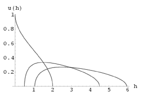
Figure 3: Plot of $u(h)$ vs. h for Solution Class 1. The value of $\xi$ increases from 0.5 as one goes from the leftmost graph to the right.

The support of $u(h)$ as well as $k^{\prime}$ is determined by expanding $H(h)$ for large $h$ and matching with property (iii) of $H(h)$ listed above.

$$H(h\rightarrow\infty)\sim\ln\left[{(\sqrt{q}+\sqrt{p})^{2}\over 4\ \xi}\right]+{(\sqrt{p}-\sqrt{q})^{2}\over 2}{1\over h}+\left(\sqrt{qp}+{3\over 4}\right){1\over h^{2}}\ .$$ (64)

We therefore obtain

$$\sqrt{q} = \sqrt{\xi}-{1\over\sqrt{2}},$$ (65)

$$\sqrt{p} = \sqrt{\xi}+{1\over\sqrt{2}}$$ (66)

and

$$k^{\prime}=\sqrt{qp}+{1\over 4}$$ (67)

which implies

$$a_{1}={4\xi^{2}\over 4\xi-1}$$ (68)

using the definition $\xi^{2}=a_{1}k^{\prime}$. Since $q$ is a real positive quantity, Eq.65 implies that this solution branch exists for $\xi\geq{1\over 2}$. From Eq.68, we therefore conclude that this class of solutions only exist for $a_{1}\geq 1$.

4.2.2 Solution Class 2:

Using the ansatz 58 the saddle equation becomes,

$${-\hskip-12.0pt}\int_{q}^{p}dh^{\prime}{\tilde{u}(h^{\prime})\over h-h^{\prime}}=\ \ln\left[{h\over\xi}\right]-\ln\left[{h\over h-q}\right]{\hskip 14.22636pt}\textrm{\tiny\large where,}\ h\in[q,p]\ .$$ (69)

The full resolvent $H(h)$ now takes the form,

$$H(h)=\ln\left[{h\over h-q}\right]+\int_{q}^{p}dh^{\prime}{\tilde{u}(h^{\prime})\over h-h^{\prime}}\ .$$ (70)

$H(h)$ can once again be written as a contour integral,

$$H(h)=\ln\left[{h\over h-q}\right]-\sqrt{(h-p)\ (h-q)}\oint{ds\over 2\pi i}{\ln\left(s/\xi\right)-\ln\left[s/(s-q)\right]\over(s-h)\sqrt{(s-p)\ (s-q)}}\ .$$ (71)

The contour is shown in fig 4.

Figure 4: Contour for Solution Class 2

Carrying out the integration gives the answer

$$H(h)=\ln\left[{h\over\xi}\right]+\ln\left[{\sqrt{p}-\sqrt{q}\over\sqrt{p}+\sqrt{q}}\right]+\ln\left[{h+\sqrt{qp}-\sqrt{(h-1)^{2}-4\xi^{2}}\over h-\sqrt{qp}+\sqrt{(h-1)^{2}-4\xi^{2}}}\right]\ .$$ (72)

Hence, the Young Tableaux density is given by,

$$\tilde{u}(h)={1\over\pi}\textrm{\tiny\large cos}^{-1}\left[{h-1\over 2\xi}\right]\ .$$ (73)

Fig.5 shows the plot of $\tilde{u}(h)$ vs. h for this solution class.

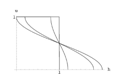
Figure 5: Plot of $\tilde{u}(h)$ vs. h for Solution Class 2. The value of $\xi$ decrease from 0.5 to 0 as one goes from the rightmost to the leftmost graph.

As before, expanding $H(h)$ for large $h$ we find the values of $q$, $p$ and $k^{\prime}$ as follows,

$$q = 1-2\xi\ ,$$ (74)

$$p = 1+2\xi$$ (75)

and

$$k^{\prime}=\xi^{2}\ .$$ (76)

From the definition $a_{1}k^{\prime}=\xi^{2}$ we obtain

$$\textrm{\tiny\large either}\ \xi = 0$$

$$\textrm{\tiny\large or},a_{1} = 1.$$ (77)

The former implies the uniform distribution

$$u(h)=1\ \ \ \ h\in[0,1].$$ (78)

This is therefore a saddlepoint for any value of $a_{1}$. This is in fact the density corresponding to the trivial representation $n_{i}=0$.

The latter corresponds to a family of saddlepoints labelled by $\xi$ which exists only at $a_{1}=1$. From Eq. (74) it is clear that this family exists for $\xi\leq 1/2$.

To summarise, we see that there are three different saddlepoint configurations of Young Tableau densities.

• The trivial representation corresponding to the uniform distribution for $u(h)$, Eq. 78. This exists for any value of $a_{1}$, i.e. for any temperature.

• The continuous family Eq. 73 which exists only for $a_{1}=1$. Here a finite fraction of the rows of the Young Tableau are empty.

• The representation Eq. 63 which exists only for $a_{1}>1$, i.e. only for high enough temperature. Now all the $N$ rows of the Young Tableaux are filled.

We see that the saddlepoints are exactly in correspondence with the saddlepoints of the eigenvalue density, as summarised in Sec.2.2. We will now indeed verify that the large $N$ free energy of these saddle points is also exactly the same as that seen from the eigenvalue density analysis.

4.3 The Free Energy of the Free Theory

In the large $N$ limit the free energy of the partition function Eq. 49 is given by,

$$F=-T\ln Z\ =N^{2}TS_{\textrm{\tiny eff}}^{0}\ .$$ (79)

where $S_{\textrm{\tiny eff}}^{0}$ is the value of effective action at the (dominant) saddlepoint. The effective action given in 50 can be re-expressed as a functional of $u(h)$

$$-S_{\textrm{\tiny eff}}=\int_{h_{L}}^{h_{U}}dh{-\hskip-12.0pt}\int_{h_{L}}^{h_{U}}dh^{\prime}u(h)u(h^{\prime})\ln|h-h^{\prime}|-2\int_{h_{L}}^{h_{U}}dh\ u(h)\ h\ \ln[h]+k^{\prime}+1+k^{\prime}\ \ln[a_{1}k^{\prime}].$$ (80)

We only need to evaluate this functional on the different saddlepoint configurations we have found. In evaluating the expressions it is useful to use the corresponding saddlepoint equations to eliminate the quadratic term in $u(h)$ in the effective action. We thus obtain:

• Solution Class 1: Using the saddle equation Eq. (60), $S_{\textrm{\tiny eff}}$ becomes

  $$-S_{\textrm{\tiny eff}}^{0}=-\int_{q}^{p}dhu(h)h\ln h+\left(\xi-{3\over 4}\right)\ln[\xi]+{1\over 2}+{\cal C}_{1}\ ,$$ (81)

  where the constant ${\cal C}_{1}$ is given by,

  $${\cal C}_{1}={1\over 2}\ln[\xi/2]+\xi-{1\over 2}.$$ (82)

  Evaluating the integral (details can be found in Appendix A) gives finally for the effective action,

  $$F=N^{2}TS_{\textrm{\tiny eff}}^{0}=-N^{2}T\left[\xi-{1\over 2}\ln(2\xi)-{1\over 2}\right]\leq 0.$$ (83)

  This exactly agrees with the free energy computed in [8] for the deconfined phase saddlepoint which was quoted in Sec.2.2.

• Solution class 2 :

  Here the free energy is easy to compute since we have a continuous family labelled by $\xi$ which are all saddlepoints and thus must have the same free energy when $a_{1}=1$. In particular the constant configuration Eq.78 is a limiting member of this family for which the effective action is readily computed to be zero. Therefore the entire family of saddlepoints in Eq.73 must have zero free energy. This is explicitly verified in appendix A. Once again this matches with the results of the eigenvalue analysis for the confined phase saddlepoint.

We see from this that there is an exchange of dominance of the saddle points at $a_{1}\geq 1$, where one gets a new saddlepoint Eq.63, which has less free energy compared to the uniform density saddlepoint that exists for all values of $a_{1}$. Therefore as the temperature increases we get a transition when the saddlepoint switches giving rise to the confinement-deconfinement transition. We see that this is nothing bu the analogue of the Douglas-Kazakov transition in our approach. We have thus reproduced the usual saddlepoints as well as the phase diagram of the zero coupling Yang-Mills theory from our method of taking the large $N$ limit of the exact solution.

4.4 Extension to Non-zero Coupling

The general interacting unitary matrix model Eq.7 for perturbative gauge theory can also be solved exactly using the technique of Sec.3 and a large $N$ limit can then be taken along the lines described in this section. However, the analysis is going to be technically much more involved. But as described in Sec.2, the essentials of the physics is in any case captured by models involving only ${\rm Tr}U$. In particular, the $(a,b)$ model Eq.10 already does a good job in getting the detailed form of the Hawking-Page phase diagram[10]. Here we will sketch how its exact solution Eq.35 shows all the features described in Sec.2.2 when we take the large $N$ limit as described in this section.

Let’s write the answer Eq.35 as

$$Z(a_{1},b_{1}) = \sum\limits_{k=0}^{\infty}\sum\limits_{l=0}^{k/2}{a_{1}^{k-2l}b_{1}^{l}k!\over N^{2l}l!(k-2l)!}\sum\limits_{\{n_{i}\}}{d_{\{n_{i}\}}^{2}(S_{k})\over k!}\delta(k-\Sigma_{i}n_{i})$$ (84)

$$= \sum\limits_{k=0}^{\infty}f(k)\sum\limits_{\{n_{i}\}}{d_{\{n_{i}\}}^{2}(S_{k})\over k!}\delta(k-\Sigma_{i}n_{i})\ ,$$

where, as usual, $\{n_{i}\}$ label the number of boxes in the Young Tableaux and

$$f(k)=\sum\limits_{l=0}^{k/2}{a_{1}^{k-2l}b_{1}^{l}k!\over N^{2l}l!(k-2l)!}.$$ (85)

Since the total number of boxes $k$ is of order $N^{2}$, we can replace the sum in Eq. 85 by the saddlepoint value. Doing this gives

$$f(k)={k\over 2}\left({a_{1}\over 1-x}\right)^{k}e^{-{kx\over 2}}\equiv{k\over 2}{\tilde{a}_{1}}^{k}$$ (86)

where $x$ is determined by the equation

$${x\over(1-x)^{2}}={2b_{1}k^{\prime}\over a_{1}^{2}}$$ (87)

with $k=N^{2}k^{\prime}$. Therefore the partition function

$$Z(a_{1},b_{1})=\sum\limits_{\{n_{i}\}}{k\over 2}{\tilde{a}_{1}}^{k}\ {d_{\{n_{i}\}}^{2}(S_{k})\over k!},$$ (88)

(with $k=\sum_{i}n_{i}$) takes essentially the same form as Eq.40 except that we have ${\tilde{a}_{1}}$ instead of $a_{1}$.

We can now take the large $N$ limit as before to obtain

$$Z(a_{1},b_{1})=\int[dh(x)]\ \textrm{\tiny\large e}^{-N^{2}S_{\textrm{\tiny eff}}},$$ (89)

where $S_{\textrm{\tiny eff}}$ is the same as in Eq.50 with the replacement of $a_{1}$ by ${\tilde{a}_{1}}$.

Since ${\tilde{a}_{1}}$ depends on $k^{\prime}$ or $h(x)$ (see 86 and below), the saddle equations are modified a bit. Taking into account this additional dependence on $h(x)$, the saddle equation becomes,

$${-\hskip-12.0pt}\int_{h_{L}}^{h_{U}}dh^{\prime}{u(h^{\prime})\over h-h^{\prime}}=\ln\left[h(x)\over\tilde{\xi}\right]\ \ \textrm{\tiny\large where}\ \ \tilde{\xi}^{2}=\tilde{a}_{1}k^{\prime}\textrm{\tiny\large e}^{x\over 2}.$$ (90)

Since the saddle equations are of the same form as Eq.55, (with the replacement of $\xi$ by $\tilde{\xi}$) the saddlepoint configurations for the Young Tableaux density are also the same in form. Namely, we obtain the three different configurations of Sec.4.2. In fact, we can redo this analysis for the class of models Eq.8 for which the exact solution was given in Eq.37. This is performed in Appendix B. We see from the analysis there that the saddlepoint equations give once again the same saddlepoint configurations. Moreover, we obtain the same Hartree-Fock equations as Eq. 22 and Eq. 23. Thus the phase diagram turns out to be the same as that given by the eigenvalue density analysis. For instance in the case of the $(a,b)$ model we find

• A low temperature saddlepoint which is characterised by $\tilde{\xi}=0$ which is the uniform distribution corresponding to thermal $AdS$. This has zero free energy.

• Then there is a saddlepoint of the form Eq. 73 when $\tilde{\xi}^{2}=k^{\prime}$ i.e. ${\tilde{a}_{1}}e^{x\over 2}=1$ and $\tilde{\xi}\leq{1\over 2}$. This implies that

  $$\tilde{\xi}^{2}={1-a_{1}\over 2b_{1}}\leq{1\over 4}\ .$$ (91)

  This is actually the unstable saddlepoint corresponding to the small black hole (in the phase where it is to be viewed as an excited string state) and has positive free energy

  $$F=N^{2}T{(1-a_{1})^{2}\over 4b_{1}}\ .$$ (92)

  This saddlepoint exists in a temperature range $T_{c}\leq T\leq T_{H}$.

• Finally there is the saddlepoint of the form Eq. 63 which obeys

  $${a_{1}\over 1-x} = {4\tilde{\xi}^{2}\over 4\tilde{\xi}-1}$$

  $$\textrm{\tiny\large and}\ \ k^{\prime} = \tilde{\xi}-{1\over 4}\ .$$ (93)

  The two solutions to this equation give rise to the BBH as well as the SBH (in the actual black hole regime). The BBH solution exists for all temperatures greater than the minimum $T_{0}$ for which this solution exists. While the (gapped) SBH solution exists in the interval $T_{o}\leq T\leq T_{c}$. At $T_{c}$ which corresponds to $\tilde{\xi}={1\over 2}$, this solution goes over into the ungapped solution. The free energy in this phase is given by,

  $$F=-N^{2}T\left[\tilde{\xi}-{1\over 2}\ln[2\tilde{\xi}]-{1\over 2}-b_{1}\left(1-{1\over 4\tilde{\xi}}\right)^{4}\right].$$ (94)

One of the points to note in our analysis is that the saddle configurations for $u(h)$ are all of the same form as in the free theory. It is only that $\xi$ is a different function of the temperature. This is a mirror of the same phenomenon in the eigenvalue density analysis that the functional form of the saddle configurations of $\sigma(\theta)$ are not changed as one turns on the perturbative coupling. This robust character of the saddle point configurations is a positive indication in trying to extract universal features from these results.

Finally, we should mention that the extension to non-zero charges also follows in a straightforward way. As argued in [21], the effective matrix model has a logarithmic term which results in there no longer being a uniform eigenvalue density saddle point corresponding to thermal $AdS$. In our approach, as argued in Appendix B for a general matrix model of the form Eq.7, we find the same saddle point equations as in the eigenvalue analysis and thus the same phase diagram.

5 Free Fermionic Phase Space Description

5.1 Relation between the Young Tableaux and Eigenvalue distributions

Our analysis of the exact answer has been very different from the usual eigenvalue analysis reviewed in Sec.2. It turns out, rather remarkably, that there is nevertheless, a simple relationship between the saddlepoint configurations $u(h)$, in both the high and low temperature phases, with the corresponding saddlepoint eigenvalue densities. We will now describe this relation.

Consider first the low temperature saddlepoint $u(h)=1$. The corresponding saddlepoint for the eigenvalue density is $\sigma(\theta)={1\over 2\pi}$. From the graph of these two distributions, we notice that they are functional inverses of each other (flip the horizontal and vertical axes of one to get the other). In other words, we can make the identification

$$u = {\theta\over\pi}$$

$${h\over 2\pi} = \sigma(\theta)\ .$$ (95)

This case may seem a little trivial, so let us consider the family of saddlepoints that correspond to the unstable small black hole Eq.73

$$u(h)={1\over\pi}\textrm{\tiny\large cos}^{-1}\left[{h-1\over 2\xi}\right]{\hskip 22.76228pt}h\in[q,p];\ \ 2\xi\leq 1\ .$$ (96)

together with $u(h)=1$ for $h\in[0,p]$. Applying relations 5.1 to this case, we get immediately $\sigma(\theta)={1\over 2\pi}(1+2\xi\cos\theta)$ which is the same as Eq.17. Thus the identification holds in this case. The two distributions are again functional inverses of each other.

We finally come to the non-trivial saddlepoint corresponding to the big black hole Eq.63

$$u(h)={1\over\pi}\textrm{\tiny\large cos}^{-1}\left[{h-1\over 2\xi}+{\left(\xi-{1\over 2}\right)^{2}\over 2\xi\ h}\right]\ \ \ \ h\in[q,p]\ .$$ (97)

In this case, we have to be more careful. We see from the plot of $u(h)$ that the functional inverse is ambiguous. For a given value of $u$, there are two values of $h$. This can be directly seen from the fact that Eq.97 implies the quadratic relation

$$h^{2}-\left[1+2\xi\cos\left(\pi u(h)\right)\right]h+\left(\xi-{1\over 2}\right)^{2}=0\ .$$ (98)

If we take the difference between the two solutions $h_{+}$ and $h_{-}$, we obtain

$$h_{+}-h_{-}=2\sqrt{2\xi}\sqrt{1-2\xi\textrm{\tiny\large sin}^{2}\left({\pi u\over 2}\right)}\textrm{\tiny\large cos}\left({\pi u\over 2}\right)\ .$$ (99)

We see that if we define

$$\textrm{\tiny\large sin}^{2}{\theta_{0}\over 2}={1\over 2\xi}$$ (100)

and modify the identifications Eq.5.1 to

$$u = {\theta\over\pi}$$

$${h_{+}-h_{-}\over 2\pi} = \sigma(\theta)\ ,$$ (101)

then we obtain precisely the eigenvalue distribution in Eq.18

$$\sigma(\theta)={1\over\pi\textrm{\tiny\large sin}^{2}\left({\theta_{0}\over 2}\right)}\sqrt{\textrm{\tiny\large sin}^{2}\left({\theta_{0}\over 2}\right)-\textrm{\tiny\large sin}^{2}\left({\theta\over 2}\right)}\textrm{\tiny\large cos}\left({\theta\over 2}\right)\ .$$ (102)

5.2 Fermionic Phase Space

The relations Eq.5.1 and 5.1 between the saddlepoint eigenvalue densities and the young tableau densities have a very natural interpretation in terms of a free fermionic picture. This fermionic picture is suggested by the fact that the eigenvalues of the holonomy matrix behave like fermions. At the same time, the representations of $U(N)$ also have an interpretation in the language of non-interacting fermions with the number of boxes of the Young tableaux being like the momentum (See [24], for example). This suggests that the eigenvalue density is like a position distribution while the Young Tableau density is like a momentum distribution. Therefore, it is natural to consider a phase space distribution which gives rise to these individual distributions. In the classical (i.e. large $N$) limit, we can describe this system of $N$ fermions in terms of an incompressible fluid occupying a region of the two dimensional phase space (see [30] for a recent overview and references to the large literature on the subject).

Therefore let us assume that the saddlepoints are all described by some configuration in phase space, i.e. some region $R$ of the two dimensional plane such that the phase space density $\rho(h,\theta)$ obeys

$$\rho(h,\theta) = {1\over 2\pi}\ ;\ \ \ (h,\theta)\in R$$ (103)

$$= 0\ ;\ \ \ {\rm otherwise}.$$

We can then define the partial densities

$$u(h) = \int_{-\pi}^{\pi}\rho(h,\theta)d\theta$$

$$\sigma(\theta) = \int_{0}^{\infty}\rho(h,\theta)dh$$ (104)

where the first integral is at constant $h$ and the second at constant $\theta$. Note that

$$\int\rho(h,\theta)dhd\theta=1\ .$$ (105)

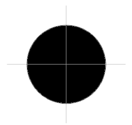
Figure 6: Phase space distribution for Thermal AdS: $\xi$ =0

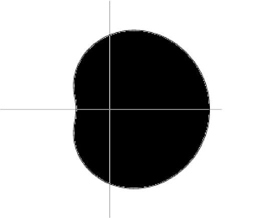
Figure 7: Phase space distribution for SBH in ungapped phase: $\xi$ =0.4

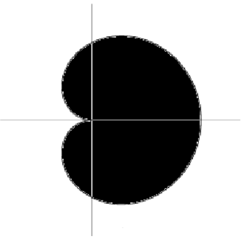
Figure 8: Phase space distribution at GWW transition point : $\xi=0.5$

Let us now take the boundary of the region $R$ to be defined by a curve $C(h,\theta)=0$.We now see that there can be different situations depending on whether the solution $h=h(\theta)$ is single valued or multiple valued. Thus for a single valued $h=h(\theta)$, we see from Eqs.103 and 5.2 that the identification Eq.5.1 follows. When we have multiple values for the solution $h(\theta)$ then the identification between the different densities is a little more non-trivial. For instance, when we have two solutions $h_{+}(\theta)$ and $h_{-}(\theta)$ with $h_{+}\geq h_{-}$, then it follows from Eqs.103, 5.2 that the relation between the young tableaux density and the eigenvalue densities is that in Eq.5.1. Thus we have an interpretation for the relationships that we observed in the previous subsection.

We therefore see that the large $N$ saddlepoints of the gauge theory effective action, which correspond to the Thermal AdS, the small black hole and the big black hole can each be thought of in terms of a particular configuration in a free fermionic phase space. There is a particular shape associated to each of them. This shape, which is determined by the curve $C(h,\theta)=0$, can, in general, only be inferred from the knowledge of both $\sigma(\theta)$ and $u(h)$. For the different saddlepoints that we have discussed, the particular shapes are given in Figs.6-9. We have plotted the regions in polar coordinates $(r,\theta)$ after making the identification in footnote 13.

The shape corresponding to thermal $AdS$ is a disk $h(\theta)=1$ (Fig. 6) which is exactly like that in the Lin, Lunin, Maldacena description for global $AdS$. For the big black hole we have a shape Fig. 9 which corresponds to a double valued $h(\theta)$. The equation of the curve is given by, Eq. 98 with $\pi u(h)$ replaced by $\theta$. Note that the origin of phase space is not contained in this region. For the unstable saddlepoint (SBH) we have the black hole regime where the shape is qualitatively the same as the BBH, except that it is closer to the origin. At the temperature $T_{c}$, the shape continuously changes to that in Fig.8. The excited string state beyond this transition occupies a region which includes the origin given by the curve $h(\theta)=1+2\xi\cos\theta$ (Fig. 7). We observe that the shapes are qualitatively of two different kinds with the limiting shape $h={r^{2}\over 2}=(1+\cos\theta)$ at the GWW transition point that separates the two classes. Note that the boundary of the limiting configuration is a separatrix between two different kinds of trajectories in the fermi sea.

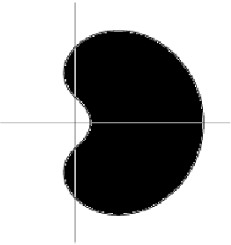
Figure 9: Phase space distribution for SBH (in the gapped phase)/BBH

6 Conclusions

We have studied thermal gauge theory by evaluating its partition function at finite $N$. Taking the large $N$ limit of the full answer gives us a new perspective on some already known facts about the phase diagram of the gauge theory. The various phases and the transitions between them can be viewed in terms of different dominant representations of $U(N)$ that contribute to the partition function. They are obtained as saddlepoints of an effective functional, $S[u(h)]$ (like that given in Eq.80) of a young tableau density. These representations can be viewed as excitations of a one dimensional fermi sea whose ground state corresponds to (thermal) AdS. In fact, a complete picture emerges when we combine the saddlepoint representation $u(h)$ with the saddlepoint $\sigma(\theta)$ of the eigenvalue density analysis. One obtains a phase space picture which neatly combines both these answers into a single two dimensional region with uniform density $\rho(h,\theta)$. An important point to emphasise is that in general, one needs both $u(h)$ and $\sigma(\theta)$ to obtain the curve $C(h,\theta)=0$ which delineates the region $R$ of phase space which is occupied. In a way, as we have seen, $u(h)$ is more basic since it contains the information to reconstruct $\sigma(\theta)$ through Eq.5.1 but not vice versa.

This suggests that it is more natural to look for a description of the dynamics directly in terms of the phase space density $\rho(h,\theta)$. In particular, it would be nice to find a phase space functional $S[\rho(h,\theta)]$ which reduces to the two different functionals $S[u(h)]$ and to $S[\sigma(\theta)]$ on appropriately integrating out. It would seem that the formalism reviewed for example in [30], would be the appropriate one.

Such a formulation is likely to help in moving towards the goal of reconstructing the local theory in the bulk with all its redundancies. Note that the configurations we are considering in the thermal history are all $S^{3}$ invariant. Thus the only non-trivial directions in the bulk are those of the thermal $S^{1}$ and the radial direction. It is tempting to identify these two directions with the phase space directions of the fermions. In fact, the eigenvalues of the fermions can be viewed as positions on the T-dual to the thermal circle and the momenta should correspond to the radial direction as per the usual AdS/CFT correspondence. As a first step it would be nice to see how the topology of the bulk is encoded in the geometry of the phase space regions corresponding to the different saddlepoints. Note that we argued that the shape of the regions is fairly robust against coupling effects and so should be telling us something generic about the bulk geometries even when they are subject to all kinds of $\alpha^{{}^{\prime}}$ corrections.

It may seem a little confusing to talk about phase space without talking about time. But since we are describing euclidean gravity configurations in terms of euclidean gauge theory, time does not enter directly. A closely similar situation arises in the study of Euclidean $2d$ Yang-Mills theory on the torus. Its free fermion representation was interpreted [26] in terms of contributions from different ”baby universe” saddle points of the Euclidean gravity partition function of the dual geometry (in this case a 4d extremal black hole in an ${\cal N}=2$ theory)[27].

As mentioned in the introduction, the LLM scenario was one of the inspirations for many of these ideas. It would be nice to see if there was a concrete connection to be made between those cases and those studied here. At first sight they seem to be very different. However one possible link between them is that unitary matrix models very similar to those studied here give the partition functions that count BPS states. In fact, it would be nice to apply our finite $N$ answers for these models to these countings.

Another interesting direction to generalise might be to the gauge theory on spatial sections which are for instance, $S^{1}\times R^{2}$ rather than $S^{3}$. We now have a matrix quantum mechanics [28]. Toy matrix models for this case have been studied for example in [29]. In these cases a free fermionic description has been employed to study the matrix quantum mechanics.

Acknowledgement: We benefitted very much from conversations with J. R. David, A. Dhar, S. Minwalla, K. S. Narain and S. Wadia. We also appreciate helpful comments by O. Aharony, S. Minwalla and S. Wadia on the draft. One of us (R.G.) also acknowledges the hospitality of IFT, Sao Paulo, where a portion of this work was completed. We also thank the participants of the ISM07 workshop on string theory for their comments. Finally, we are both beholden to the people of India for the unstinting support lent to fundamental research.

——————————————————–

Appendix

Appendix A Details of the Evaluation of the Free Energy

A.1 Free Energy for solution class 1

The effective action is given by

$$-S_{\textrm{\tiny eff}}=\int_{h_{L}}^{h_{U}}dh{-\hskip-12.0pt}\int_{h_{L}}^{h_{U}}dh^{\prime}u(h)u(h^{\prime})\ln|h-h^{\prime}|-2\int_{h_{L}}^{h_{U}}dh\ u(h)\ h\ln(h)+k^{\prime}+1+k^{\prime}\ln(a_{1}k^{\prime})$$ (106)

For solution class 1, $h_{L}=q$ and $h_{U}=p$. $u(h)$ has support only for $q\leq h\leq p$.

Using the following saddle equation of motion we can replace the double integration by a single integration,

$${-\hskip-12.0pt}\int_{q}^{p}dh^{\prime}\ln[h-h^{\prime}]\ u(h^{\prime})=h\ln\left[{h\over\xi}\right]-h+{\cal C}_{1}\ .$$ (107)

Hence the effective action becomes,

$$-S_{\textrm{\tiny eff}}^{0}=-\int_{q}^{p}dhhu(h)\ln[h]+\xi\ln[\xi]-{3\over 4}\ln[\xi]+{1\over 2}+{\cal C}_{1}\ .$$ (108)

The constant ${\cal C}_{1}$ can be evaluated from the equation 107 at $h=p$.

$${\cal C}_{1}=p+p\ln\left[{p\over\xi}\right]+\int_{q}^{p}dh^{\prime}\ln[p-h^{\prime}]\ u(h^{\prime})\ .$$ (109)

After some algebra we find,

$$\int_{q}^{p}dhhu(h)\ln[h]=\xi\ln[\xi]+{1\over 4}\ln[\xi]+{1\over 2}$$ (110)

and

$${\cal C}_{1}={1\over 2}\ln[\xi/2]+\xi-{1\over 2}\ .$$ (111)

Finally we get,

$$S_{\textrm{\tiny eff}}^{0} = \ln[\xi]-{\cal C}_{1}$$ (112)

$$= -\left[\xi-{1\over 2}\ln[2\xi]-{1\over 2}\right]\ .$$

A.2 Free Energy for solution class 2

The effective action for the solutions in class 2 is given by,

$$-S_{\textrm{\tiny eff}}=\int_{0}^{p}dh{-\hskip-12.0pt\int}_{0}^{p} dh^{\prime} u(h)u(h^{\prime})\ln|h-h^{\prime}|-2\int_{0}^{p}dhu(h)h\ln(h)$$ (113)

$$+ k^{\prime}+1+k^{\prime}\ln(a_{1}k^{\prime}).$$

Breaking the $h$ integration into two pieces, we can write the effective action as,

$$-S_{\textrm{\tiny eff}} = \int_{0}^{q}dh{-\hskip-12.0pt\int}_{0}^{p}dh^{\prime}u(h)u(h^{\prime})\ln|h-h^{\prime}|+\int_{q}^{p}dh{-\hskip-12.0pt\int}_{0}^{q}dh^{\prime}u(h)u(h^{\prime})\ln|h-h^{\prime}|$$ (114)

$$- 2\int_{0}^{p}dhu(h)h\ln(h)+k^{\prime}+1+k^{\prime}\ln(a_{1}k^{\prime}).$$

In the second term on the right hand side, one can use the saddle equation Eq. (55) with $h_{L}=0$ and $h_{U}=p$. This gives

$$\int_{q}^{p}dh{-\hskip-12.0pt\int}_{0}^{p}dh^{\prime}u(h)u(h^{\prime})\ln|h-h^{\prime}|=\int_{q}^{p}dhu(h)\left(h\ln[h]-h\ln[\xi]-h-{\cal C}_{2}\right),$$ (115)

where the constant ${\cal C}_{2}$ is given by,

$${\cal C}_{2}=p-p\ \ln\left[{p\over\xi}\right]+{-\hskip-12.0pt\int}_{0}^{p}dh^{\prime}\ u(h^{\prime})\ \ln|h-h^{\prime}|\ .$$ (116)

After some algebra we get,

$${\cal C}_{2}=\ln[\xi]\ .$$ (117)

Therefore

$$\int_{q}^{p}dh{-\hskip-12.0pt\int}_{0}^{p}dh^{\prime}u(h)u(h^{\prime})\ln|h-h^{\prime}| = \int_{q}^{p}dhhu(h)\ln[h]$$ (118)

$$- (1+\ln[\xi])\left(k^{\prime}+{1\over 2}-{q^{2}\over 2}\right)+{\cal C}_{2}(1-q).$$

Calculating the first term on the right hand side of Eq. (114) we get,

$$\int_{0}^{q}dh{-\hskip-12.0pt\int}_{0}^{p}dh^{\prime}u(h)u(h^{\prime})\ln|h-h^{\prime}| = -{q^{2}\over 2}+q^{2}\ln[q]+\int_{q}^{p}dh^{\prime}h^{\prime}u(h^{\prime})\ln[h^{\prime}]$$ (119)

$$- q+\int_{q}^{p}dh^{\prime}u(h^{\prime})(q-h^{\prime})\ln[h^{\prime}-q]\ .$$

Calculating other terms in on the right hand side of Eq. (114) we finally see that the on-shell effective action in second branch vanishes. Hence the free energy in this branch is zero.

Appendix B A Class of General Matrix Model Actions

In this appendix we will generalize the result of section 4 to a generic effective action which is a function of $\textrm{\tiny\large Tr}U\textrm{\tiny\large Tr}U^{\dagger}$. We will expand the effective action in a power series in $x$, where $x=\textrm{\tiny\large Tr}U\textrm{\tiny\large Tr}U^{\dagger}$.

$$-S_{\textrm{\tiny eff}}=\sum\limits_{n=1}{a_{n}x^{n}\over N^{2(n-1)}}=N^{2}\sum\limits_{n=1}{a_{n}x^{n}\over N^{2n}}.$$ (120)

Using this form of $S_{\textrm{\tiny eff}}$, we can write

$$\textrm{\tiny\large e}^{-S_{\textrm{\tiny eff}}}=\prod\limits_{i}^{m}\sum\limits_{k_{i}=0}^{\infty}{(a_{i})^{k_{i}}\ x^{(\sum_{i=1}^{\infty}ik_{i})}\over k_{i}!N^{2(i-1)}}.$$ (121)

The partition function   is given by,

$$Z=\int[dU]\textrm{\tiny\large e}^{-S_{\textrm{\tiny eff}}},$$ (122)

can be evaluated using the methods of Sec.3 and Sec.4,

$$Z=\sum\limits_{\{k_{i}\}=0}^{\infty}{a_{1}^{k_{1}}\cdot\cdot a_{m}^{k_{m}}\over k_{1}!\cdot\cdot k_{m}!}\left[{\sum\limits_{R}d_{R}^{2}(S_{k})\over N^{2\sum\limits_{l=1}^{m}k_{l}(l-1)}}\right]\ \ ,\ \ k=\sum\limits_{l=1}lk_{l}\ .$$ (123)

Define,

$$f(k) = \sum\limits_{\{k_{i}\}=0}^{\infty}{a_{1}^{k_{1}}\cdot\cdot a_{m}^{k_{m}}\cdot\over k_{1}!\cdot\cdot k_{m}!\cdot}{k!\over N^{2\sum\limits_{l=1}k_{l}(l-1)}}$$ (124)

$$= \sum\limits_{\{k_{i}\}=0}^{\infty}\textrm{\tiny\large e}^{G(\{k_{i}\})}\ ,$$

where $G(\{k_{i}\})$ is given by,

$$G(\{k_{i}\})=\sum\limits_{i=1}k_{i}\ln[a_{i}]-\sum\limits_{i=1}^{m}\left(k_{i}\ln[k_{i}]-k_{i}\right)+k\ln[k]-k-2\sum\limits_{i=1}^{m}k_{i}(i-1)\ln[N].$$ (125)

In the large $N$ limit the partition function  receives its dominant contribution only from the extremum value of $G$. Minimising $G$ with respect to $k_{i}$, remembering to introduce a Lagrange multiplier for the constraint $\sum\limits_{i=1}ik_{i}=k$, we get,

$$k_{i}^{\prime}=a_{i}\beta^{i}\ ,$$ (126)

where $k_{i}^{\prime}={k_{i}\over N^{2}}$ and $\beta=\textrm{\tiny\large e}^{-(\alpha+2\ln N)}$ where $\alpha$ is the Lagrange multiplier enforcing the constraint.

$\beta$ is determined through the following relation,

$$k^{\prime} = \sum\limits_{i=1}^{\infty}ik_{i}^{\prime}$$ (127)

$$= \sum\limits_{i=1}ia_{i}\beta^{i}$$

$$= \beta\tilde{S}^{\prime}(\beta)\ ,$$

where $\tilde{S}^{\prime}(\beta)$ is given by,

$$\tilde{S}(\beta)=\sum\limits_{i=1}a_{i}\beta^{i}\ .$$ (128)

Once we fix the undetermined multiplier, then $G$ can be written as,

$${G\over N^{2}}=k^{\prime}\ln[k^{\prime}]-k^{\prime}-k^{\prime}\ln[\beta]+\tilde{S}(\beta)\ .$$ (129)

Hence $f(k)$ is given (upto multiplicative factors which are unimportant in the large $N$ limit).

$$f(k)\propto\textrm{\tiny\large e}^{N^{2}(k^{\prime}\ln[{k^{\prime}\over\beta}]-1)}\textrm{\tiny\large e}^{N^{2}\tilde{S}(\beta)}\ .$$ (130)

So the partition function  can be written as,

$$Z=\sum\limits_{k=0}^{\infty}{\tilde{a}^{k}\over k!}\sum\limits_{R}d_{R}^{2}(S_{k})\ ,$$ (131)

where $\tilde{a}^{k}=\textrm{\tiny\large e}^{k\ln[k^{\prime}/\beta]-k+N^{2}\tilde{S}(\beta)}$. Like before we will write the partition function  in the following form,

$$Z=\int[dh(x)]\exp[-N^{2}S_{\textrm{\tiny eff}}],$$ (132)

where $S_{\textrm{\tiny eff}}$ is given by,

$$-S_{\textrm{\tiny eff}} = {-\hskip-12.0pt}\int_{0}^{1}dx\int_{0}^{1}dy\ln|h(x)-h(y)|$$ (133)

$$- 2\int_{0}^{1}dxh(x)\ln h(x)\ +\ k^{\prime}\ln\left({\tilde{a}\ k^{\prime}}\right)+k^{\prime}+1\ .$$

Hence the saddlepoint equation is given by,

$${-\hskip-12.0pt}\int_{h_{L}}^{h_{U}}dh^{\prime}{u(h^{\prime})\over h-h^{\prime}}=\ln({h\over\tilde{\xi}}),$$ (134)

where $\tilde{\xi}$ is given by,

$$\tilde{\xi}^{2}=k^{\prime}\tilde{S}^{\prime}(\beta)\ .$$ (135)

For this generic effective action the solutions of the saddle equation are given by,

$$\beta\tilde{S}^{\prime}(\beta) = \beta{\hskip 65.44142pt}\textrm{\tiny\large for}\ \ \beta\in[0,{1\over 4}]$$

$$\tilde{S}^{\prime}(\beta) = {1\over 4\sqrt{\beta}(1-\sqrt{\beta})}\ \ \textrm{\tiny\large for}\ \ \beta\in[{1\over 4},1]\ .$$ (136)

For $\beta\in[0,{1\over 4}]$, $\xi=\sqrt{\beta}$ and for $\beta\in[{1\over 4},1]$, $\xi={1\over 4(1-\sqrt{\beta})}$.

These equations are identical to those obtained by the Hartree-Fock analysis of eigenvalue density Eq. 22 and Eq. 23.

References

- [1] H. Lin, O. Lunin and J. M. Maldacena, “Bubbling AdS space and 1/2 BPS geometries,” JHEP 0410, 025 (2004) [arXiv:hep-th/0409174].
- [2] G. Mandal, “Fermions from half-BPS supergravity,” JHEP 0508, 052 (2005) [arXiv:hep-th/0502104].
- [3] L. Grant, L. Maoz, J. Marsano, K. Papadodimas and V. S. Rychkov, “Minisuperspace quantization of ’bubbling AdS’ and free fermion droplets,” JHEP 0508, 025 (2005) [arXiv:hep-th/0505079].
- [4] E. Witten, “Anti-de Sitter space, thermal phase transition, and confinement in gauge theories,” Adv. Theor. Math. Phys. 2, 505 (1998) [arXiv:hep-th/9803131].
- [5] S. W. Hawking and D. N. Page, “Thermodynamics Of Black Holes In Anti-De Sitter Space,” Commun. Math. Phys. 87, 577 (1983).
- [6] B. Sundborg, “The Hagedorn transition, deconfinement and N = 4 SYM theory,” Nucl. Phys. B 573, 349 (2000) [arXiv:hep-th/9908001].
- [7] J. Hallin and D. Persson, “Thermal phase transition in weakly interacting, large N(c) QCD,” Phys. Lett. B 429, 232 (1998) [arXiv:hep-ph/9803234].
- [8] O. Aharony, J. Marsano, S. Minwalla, K. Papadodimas and M. Van Raamsdonk, “The Hagedorn / deconfinement phase transition in weakly coupled large N gauge theories,” Adv. Theor. Math. Phys. 8, 603 (2004) [arXiv:hep-th/0310285].
- [9] H. Liu, “Fine structure of Hagedorn transitions,” arXiv:hep-th/0408001.
- [10] L. Alvarez-Gaume, C. Gomez, H. Liu and S. Wadia, “Finite temperature effective action, AdS(5) black holes, and 1/N expansion,” Phys. Rev. D 71, 124023 (2005) [arXiv:hep-th/0502227].
- [11] Takehiro Azuma, Pallab Basu, Spenta R. Wadia, “Monte Carlo Studies of the GWW Phase Transition in Large-N Gauge Theories,” arXiv:0710.5873[hep-th].
- [12] M. R. Douglas and V. A. Kazakov, “Large N phase transition in continuum QCD in two-dimensions,” Phys. Lett. B 319, 219 (1993) [arXiv:hep-th/9305047].
- [13] V. A. Kazakov, M. Staudacher and T. Wynter, “Character expansion methods for matrix models of dually weighted graphs,” Commun. Math. Phys. 177, 451 (1996) [arXiv:hep-th/9502132].
- [14] D. J. Gross and A. Matytsin, “Some Properties Of Large N Two-Dimensional Yang-Mills Theory,” Nucl. Phys. B 437, 541 (1995) [arXiv:hep-th/9410054].
- [15] D. J. Gross and E. Witten, “Possible Third Order Phase Transition In The Large N Lattice Gauge Theory,” Phys. Rev. D 21 (1980) 446.
- [16] S. R. Wadia, “N = Infinity Phase Transition In A Class Of Exactly Soluble Model Lattice Gauge Theories,” Phys. Lett. B 93, 403 (1980).
- [17] L. Alvarez-Gaume, P. Basu, M. Marino and S. R. Wadia, “Blackhole / string transition for the small Schwarzschild blackhole of AdS(5) x S**5 and critical unitary matrix models,” Eur. Phys. J. C 48, 647 (2006) [arXiv:hep-th/0605041].
- [18] Morton Hamermesh, “Group Theory and its Application to Physical Problems,” Dover publications.
- [19] Michel Lasalle, ”‘Explicitation of Characters of the Symmetric Group,”’ C. R. Acad. Sci. Paris, Ser I341, 529-534 (2005).
- [20] M. Marino, “Les Houches lectures on matrix models and topological strings,” arXiv:hep-th/0410165.
- [21] P. Basu and S. R. Wadia, “R-charged AdS(5) black holes and large N unitary matrix models, Phys. Rev. D 73, 045022 (2006)” [arXiv:hep-th/0506203].
- [22] D. Yamada and L. G. Yaffe, “Phase diagram of N = 4 super-Yang-Mills theory with R-symmetry chemical potentials,” JHEP 0609, 027 (2006) [arXiv:hep-th/0602074]. T. Harmark and M. Orselli, “Quantum mechanical sectors in thermal N = 4 super Yang-Mills on R x S**3,” Nucl. Phys. B 757, 117 (2006) [arXiv:hep-th/0605234].
- [23] T. Harmark, K. R. Kristjansson and M. Orselli, JHEP 0709, 115 (2007) [arXiv:0707.1621 [hep-th]].
- [24] M. R. Douglas, “Conformal field theory techniques in large N Yang-Mills theory,” arXiv:hep-th/9311130.
- [25] X. Arsiwalla, R. Boels, M. Marino and A. Sinkovics, “Phase transitions in q-deformed 2d Yang-Mills theory and topological strings,” Phys. Rev. D 73, 026005 (2006) [arXiv:hep-th/0509002].
- [26] R. Dijkgraaf, R. Gopakumar, H. Ooguri and C. Vafa, “Baby universes in string theory,” Phys. Rev. D 73, 066002 (2006) [arXiv:hep-th/0504221].
- [27] C. Vafa, “Two dimensional Yang-Mills, black holes and topological strings,” arXiv:hep-th/0406058.
- [28] O. Aharony, J. Marsano, S. Minwalla, K. Papadodimas, M. Van Raamsdonk and T. Wiseman, “The phase structure of low dimensional large N gauge theories on tori,” JHEP 0601, 140 (2006) [arXiv:hep-th/0508077].
- [29] P. Basu, B. Ezhuthachan and S. R. Wadia, “Plasma balls / kinks as solitons of large N confining gauge theories,” JHEP 0701, 003 (2007) [arXiv:hep-th/0610257].
- [30] A. Dhar, “Bosonization of non-relativstic fermions in 2-dimensions and collective field theory,” JHEP 0507, 064 (2005) [arXiv:hep-th/0505084].
- [31] J. Kinney, J. M. Maldacena, S. Minwalla and S. Raju, “An index for 4 dimensional super conformal theories,” Commun. Math. Phys. 275, 209 (2007) [arXiv:hep-th/0510251].