Grassmannian Beamforming for MIMO Amplify-and-Forward Relaying

Abstract

In this paper, we derive the optimal transmitter/receiver beamforming vectors and relay weighting matrix for the multiple-input multiple-output amplify-and-forward relay channel. The analysis is accomplished in two steps. In the first step, the direct link between the transmitter (Tx) and receiver (Rx) is ignored and we show that the transmitter and the relay should map their signals to the strongest right singular vectors of the Tx-relay and relay-Rx channels. Based on the distributions of these vectors for independent identically distributed (i.i.d.) Rayleigh channels, the Grassmannian codebooks are used for quantizing and sending back the channel information to the transmitter and the relay. The simulation results show that even a few number of bits can considerably increase the link reliability in terms of bit error rate. For the second step, the direct link is considered in the problem model and we derive the optimization problem that identifies the optimal Tx beamforming vector. For the i.i.d Rayleigh channels, we show that the solution to this problem is uniformly distributed on the unit sphere and we justify the appropriateness of the Grassmannian codebook (for determining the optimal beamforming vector), both analytically and by simulation. Finally, a modified quantizing scheme is presented which introduces a negligible degradation in the system performance but significantly reduces the required number of feedback bits.

I Introduction

The multiple-input multiple-output (MIMO) technology provides a wireless system with a large number of degrees of freedom, which can be used for increasing the capacity and/or reliability of the wireless links. Relaying techniques, on the other hand, can extend the communication range and coverage, by supporting the shadowed users through the relay nodes, and reduce the transmission power required to reach the users far from the base station. These benefits make MIMO relaying techniques a powerful candidate for implementation in the next generation of wireless networks.

Considering a system with a single data stream and perfect channel knowledge at the receiver, several methods can be used to achieve the benefits of the MIMO link. Maximum ratio transmission and receiving (MRT-MRC) [1] is one of the simplest methods which can achieve full diversity order while providing considerable array gains compared to space-time codes [2]. This gain is obtained at the expense of the channel knowledge at the transmitter and therefore, the receiver needs to send the quantized channel information back to the transmitter. While a general purpose MMSE quantizer can be used to describe each channel matrix entry, it requires a large number of feedback bits and does not preserve the structure of the optimal beamforming vector [3]. A more efficient approach is to have a common beamforming-vector codebook with finite cardinality and send back the label of the best beamforming vector to transmitter. This codebook is designed offline and is known to the transmitter and the receiver. For the case of flat Rayleigh fading channel, the codebook design problem has been shown to be related to the Grassmannian line packing problem [4, 5, 6].

In this paper, we generalize the idea of MRT-MRC to a MIMO link with an amplify-and-forward relay station. The scenario, considered in this paper, comprises a transmitter (Tx), a receiver (Rx) and a relay which helps the transmitter to send its data to the receiver. A general information theoretic analysis of MIMO relay link has been presented in [7] and [8]. Although an efficient signaling through the relay channel requires a full-duplex relay with specific processing capabilities (e.g. encoding/decoding), amplify-and-forward (AF) relays are still attractive due to their lower complexity. Moreover, the full-duplex assumption cannot be realized by the current technology, as the input and output signals need to be separated in time or frequency at the relay. For these reasons, this paper focuses on the half-duplex AF relay system. In such a system, the transmitter sends out its symbol in the first time slot and the relay and the receiver receive their signal. In the second time slot, the transmitter remains silent and the relay multiplies its received signal by a matrix (amplification) and sends the resulting signal to the receiver. The receiver decodes the transmitted symbol based on the signals received in two consecutive slots.

The half-duplex MIMO AF scenario has been considered in [9] and [10], where the authors present different solutions for maximizing the instantaneous capacity with respect to the weighting (amplification) matrix of the relay. These papers assume no channel state information at the transmitter (CSIT) and consider uniform power allocation over the Tx antennas. The work in [11] considers the same problem with perfect CSIT and derives the optimal power allocation scheme for the transmitter and relay (without considering the Tx-Rx link). Our problem setup is different from these papers in two major aspects, listed below:

• The objective of the aforementioned references is the maximization of the instantaneous capacity. Our problem, however, can be categorized as a beamforming problem, where we optimize the Tx/Rx beamforming vectors and the relay matrix to maximize the signal-to-noise ratio (SNR) of a single data stream at the Rx output.

• The above papers assume either no channel information or complete channel information at the transmitter or the relay. Our work, however, focuses on a “limited feedback” system, where the receiver end of a link sends the properly quantized channel information back to the transmitter end.

The analysis in this paper starts by first ignoring the direct link between transmitter and receiver, where we show that the transmitter and the relay should map their symbols to the strongest right singular vectors of the Tx-relay and relay-Rx channels. For Rayleigh fading channels, these vectors are uniformly distributed on the unit sphere and therefore the Grassmannian criterion can be used separately for Tx-relay and relay-Rx codebook design.

In the second part of the paper, we include the direct link in the system model. As expected, one needs to know both Tx-relay and Tx-Rx channel matrices to determine the optimal Tx beamforming vector for this case. We first assume that such a knowledge is available (for example at the relay), and we derive the optimization problem that characterizes the optimal Tx beamforming vector. Although this problem does not appear to have an analytic solution, we are able to show that for i.i.d. Rayleigh channels the solution to this problem is uniformly distributed on the unit sphere, based on which, the appropriateness of the Grassmannian quantizer can be shown analytically.

In the next step, we relax the assumption of complete knowledge of the Tx-relay and Tx-Rx channels. Without this assumption, the Rx and relay should somehow exchange their information of the Tx-relay and Tx-Rx channels. We focus on a scheme, where the Rx quantizes the Tx-Rx channel matrix and sends it to the relay, which already knows the Tx-relay channel matrix. Assuming an ideal scalar quantizer for the singular values of the Tx-Rx channel matrix, we justify the use of the Grassmannian quantizer for quantizing the singular vectors. Finally, we present a modified quantizer, which only quantizes the strongest singular vector of the Tx-Rx channel and sends it to the relay. This quantizer requires fewer number of feedback bits and performs very close to the original quantizer.

The remainder of this paper is organized as follows. In Section II, we present a brief introduction to Grassmannian line packing problem and its connection to the MIMO beamforming codebook design. Section III presents the problem setup and the solution for the MIMO relay channel without considering the direct link. In Section IV, the beamforming codebook design problem is solved with the direct link included in the system model. The simulation results are discussed in Section V. Finally, Section VI concludes the paper.

Notations: $\mathds{R}$ and $\mathds{C}$ denote the set of real and complex numbers. Bold upper case and lower case letters denote matrices and vectors. $\mathbf{I}$ shows the identity matrix. $\mathcal{U}^{m}$ denotes the set of all unitary matrices in $\mathds{C}^{m\times m}$. $~{}~{}|\cdot|$ and $\|\cdot\|$ show the absolute value of a scalar and the Euclidean norm of a vector. $\|\cdot\|_{{}_{F}}$ denotes the Frobenius norm of a matrix. $(\cdot)^{T}$ and $(\cdot)^{H}$ denote the transpose and Hermitian of a matrix. The notation $\mathbf{\Phi}=\texttt{diag}_{m\times n}(\phi_{1},\phi_{2},\cdots,\phi_{r})$ with $r=\min\{m,n\}$ shows a rectangular diagonal matrix $\mathbf{\Phi}\in\mathds{C}^{m\times n}$ with $\mathbf{\Phi}(i,i)=\phi_{i}$ for $i=1,2,\cdots,r$ and $\mathbf{\Phi}(i,j)=0$ for $i\neq j$. For an arbitrary matrix $\mathbf{H}\in\mathds{C}^{m\times n}$, the singular value decomposition (SVD) of $\mathbf{H}$ is expressed as $\mathbf{H}=\mathbf{U}\mathbf{\Sigma}\mathbf{V}^{H}$, where $\mathbf{U}\in\mathcal{U}^{m}$ and $\mathbf{V}\in\mathcal{U}^{n}$ include the left and right singular vectors as their columns, and $\mathbf{\Sigma}=\texttt{diag}_{m\times n}(\sigma_{1},\sigma_{2},\cdots,\sigma_{r})$, where $r=\min\{m,n\}$ and $\sigma_{1}{\geq}\sigma_{2}{\geq}\cdots{\geq}\sigma_{r}{\geq}0$; if $R=\texttt{rank}(\mathbf{H})$, the first $R$ nonzero diagonal enteries of $\mathbf{\Sigma}$ are called the singular values of $\mathbf{H}$. $\mathcal{CN}(0,\mathbf{\Sigma})$ represents a circularly symmetric complex Gaussian distribution with zero mean and covariance matrix $\mathbf{\Sigma}$. Finally, $\mathrm{E}\{\cdot\}$ denotes the expectation operation.

II MIMO Beamforming Codebook Design and Grassmannian Line Packing

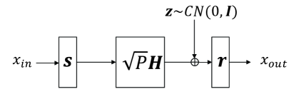
Figure 1: Single stream MIMO link with Tx and Rx beamforming.

The connection between Grassmannian line packing problem and beamforming codebook design for a Rayleigh fading channel has been independently observed in [5] and [6]. Consider the MIMO channel in Fig. 1. The transmitter maps the symbol $x_{in}$ to the antenna array using the beamforming vector $\mathbf{s}$. The signal passes through the channel $\sqrt{P}\mathbf{H}$ with complex Gaussian noise $\mathbf{z}\sim\mathcal{CN}(0,\mathbf{I})$. The receiver recovers the symbol $x_{out}$ using the receive beamforming vector $\mathbf{r}$. The matrix $\sqrt{P}\mathbf{H}\in\mathds{C}^{l\times m}$ models the flat fading channel and $m$ and $l$ are the number of the Tx and Rx antennas respectively. The entries of $\mathbf{H}$ are assumed to be independent and identically distributed according to $\mathcal{CN}(0,1)$. The coefficient $P$ is referred to as the “link signal-to-noise ratio (SNR)”. The output symbol can be expressed as

$$x_{out}=\sqrt{P}\mathbf{r}^{H}\mathbf{H}\mathbf{s}x_{in}+\mathbf{r}^{H}\mathbf{z}.$$

Assuming a transmission power constraint of $1$, satisfied by $\mathrm{E}\{|x_{in}|^{2}\}=1$ and $\|\mathbf{s}\|=1$, the received SNR $\gamma$ is:

$$\gamma=\frac{P|\mathbf{r}^{H}\mathbf{Hs}|^{2}}{\|\mathbf{r}\|^{2}},$$

which should be maximized with respect to $\mathbf{r}$ and $\mathbf{s}$. Maximization with respect to $\mathbf{r}$ is achieved by matching $\mathbf{r}=\mathbf{Hs}$, hence the optimal $\mathbf{s}$ should maximize $\gamma=P\|\mathbf{Hs}\|^{2}$. It is easy to show that the optimal $\mathbf{s}$ is the right singular vector of $\mathbf{H}$ corresponding to its largest singular value. If we denote the largest singular value and the corresponding right singular of $\mathbf{H}$ by $\sigma_{1}$ and $\mathbf{v}_{1}$, the optimal Tx beamforming vector is equal to $\mathbf{s}^{\star}=\mathbf{v}_{1}$ and the maximum SNR is $\gamma^{\star}=P\sigma_{1}^{2}$.

For the Rayleigh fading channel matrix $\mathbf{H}$, the singular vectors have been shown to be uniformly distributed on the unit sphere in $\mathds{C}^{m}$ (see [5], [12]). Therefore, a good quantizer of the optimal $\mathbf{s}$, in a sense, should place its codebook vectors uniformly on the unit sphere. This requirement can be shown to be related to the criterion used in the Grassmannian line packing problem, which we describe next.

Consider the complex space $\mathds{C}^{m}$ and let $\Omega$ be the unit sphere, $\Omega=\{\mathbf{w}\in\mathds{C}^{m}|\|\mathbf{w}\|=1\}$. Define the distance of two unit vectors to be sine of the angle between them:

$$d(\mathbf{w}_{1},\mathbf{w}_{2})=\sqrt{1-|\mathbf{w}_{1}^{H}\mathbf{w}_{2}|^{2}},$$ (1)

for $\mathbf{w}_{1},\mathbf{w}_{2}\in\Omega$. For a codebook $\mathbf{C}=\{\mathbf{w}_{1},\mathbf{w}_{2},\cdots,\mathbf{w}_{N}\}$ with $N$ distinct unit vectors, define $\delta(\mathbf{C})$ as the minimum distance of the codebook:

$$\delta(\mathbf{C})=\min_{\begin{subarray}{c}\mathbf{w}_{i},\mathbf{w}_{j}\in\mathbf{C}\\ i\neq j\end{subarray}}{d(\mathbf{w}_{i},\mathbf{w}_{j})}.$$

For a fixed dimension $m$ and codebook size $N$, the Grassmannian line packing problem [4] is that of finding a codebook $\mathbf{C}$ of size $N$ with the largest minimum distance. Many researchers have studied the solution to this problem for moderate values of $m$ and $N$ [13], [14]. However, there is no known standard way of finding these codebooks in general.

For the problem setup in Fig. 1, consider a beamforming codebook $\mathbf{C}(N,\delta)$ of size $N$ and minimum distance $\delta$. The receiver chooses the vector in this codebook that maximizes the SNR and sends the label of this vector back to the transmitter. Let $\tilde{\gamma}$ denote the resulting SNR: $\tilde{\gamma}=\max_{\mathbf{w}\in\mathbf{C}}{P\|\mathbf{H}\mathbf{w}\|^{2}}$. The authors in [5] have used the distribution of optimal beamforming vector $\mathbf{s}^{\star}$ to bound the average SNR loss as:

$$\mathrm{E}\{\gamma^{\star}\} - \mathrm{E}\{\tilde{\gamma}\}~{}\leq$$ (2)

$$P \mathrm{E}\{\sigma_{1}^{2}\}\left(1{-}N\left(\frac{\delta}{2}\right)^{2(m{-}1)}\left(1{-}\frac{\delta^{2}}{4}\right)\right),$$

where $m$ is the space dimension (number of Tx antennas). The upper bound in (2) is a decreasing function of $\delta$, for any $m>1$. Therefore, to minimize the upper bound of the SNR loss, we should maximize the minimum distance of the codebook. This is the same criterion used in the definition of the Grassmannian line packing problem and establishes the connection between the beamforming codebook design problem and the Grassmannian line packing.

Before concluding this section, we mention that the codebook design problem for the beamforming system in Fig. 1 has been generalized by [15] to the multiplexing systems, where the Tx transmits multiple substreams to the Rx. In such systems, the transmitter and receiver share a codebook of precoding matrices and the receiver sends back the label of the matrix that maximizes a certain performance criterion (e.g. the minimum substream SNR). In this paper, we take the first step in designing the limited feedback systems for beamforming over MIMO AF relay channels. The generalization of the relay problem to the case of multiple data streams is considered as the future work.

III MIMO Amplify and Forward Relay Channel without the Direct Link

In this section, we consider the MIMO amplify-and-forward (AF) relay channel without the direct link and derive the optimal transmitter/receiver beamforming vectors and relay weighting matrix in Subsection III.A. Next, we present the quantization scheme in Subsection III.B. It should be noted that if the relay performs decode-and-forward, the MIMO relay channel reduces to two MIMO links in series, therefore the optimal structure and the quantization scheme in Section I can be applied to each of the links separately. However, the derivation of the optimal unquantized scheme and designing the corresponding quantization scheme is not trivial when the relay performs amplify-and-forward.

III-A Optimal Unquantized Scheme

Consider the MIMO amplify-and-forward relay system in Fig. 2a, where the direct link between transmitter and receiver is ignored. The transmitter, the relay and the receiver are equipped with $m$, $n$ and $l$ antennas, respectively. The matrices $\sqrt{P_{1}}\mathbf{H}_{1}\in\mathds{C}^{n\times m}$ and $\sqrt{P_{2}}\mathbf{H}_{2}\in\mathds{C}^{l\times n}$ model the flat fading channels of the Tx-relay and relay-Rx links, respectively. The coefficients $P_{1}$ and $P_{2}$ are referred to as Tx-relay and relay-Rx “link SNRs”. The transmitter uses the vector $\mathbf{s}$ for beamforming. The relay multiplies its noisy received signal by the matrix $\mathbf{W}\in\mathds{C}^{l\times l}$ and sends it to the receiver. The receiver recovers its symbol using the receive beamforming (combining) vector $\mathbf{r}$. We assume power constraints equal to $1$ at the transmitter and the relay outputs.

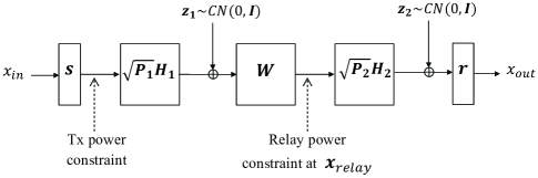
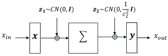
Figure 2: (a) MIMO amplify-and-forward relay channel model without the direct link, (b) The model after the change of variables $\mathbf{x}=\sqrt{P_{1}}\mathbf{V}^{H}\mathbf{H}_{1}\mathbf{s}$ and $\mathbf{y}=\sqrt{P_{2}}\mathbf{U}^{H}\mathbf{H}_{2}^{H}\mathbf{r}$.

The problem is to find the optimal $\mathbf{s}$, $\mathbf{W}$ and $\mathbf{r}$, to maximize the SNR at the receiver output subject to power constraints at the Tx and at the relay. For this problem setup, a reasonable solution is “matching”, as described below. The transmitter should map its symbol to the strongest right singular vector of $\mathbf{H}_{1}$ (as described in Section II). The relay should absorb maximum signal power by matching to the effective channel $\textbf{H}_{1}\textbf{s}$, scale the resulting (noisy) signal to meet its power constraint and transmit it through the strongest right singular vector of $\mathbf{H}_{2}$. Finally, the receiver should match to the relay-Rx link by using the strongest left singular vector of $\mathbf{H}_{2}$ as the Rx beamformer. This matching solution is depicted in Fig. 3a, in which

$$\mathbf{H}_{1}=\mathbf{A}\mathbf{\Phi}\mathbf{B}^{H},$$

$$\mathbf{H}_{2}=\mathbf{F}\mathbf{\Psi}\mathbf{G}^{H},$$ (3)

are the SVD decompositions of $\mathbf{H}_{1}$ and $\mathbf{H}_{2}$, and

$$\mathbf{A} {=} [\mathbf{a}_{1}|\mathbf{a}_{2}|\cdots|\mathbf{a}_{n}]\in\mathcal{U}^{n},$$ F = [f_1—f_2—⋯—f_l]∈U^l,

$$\mathbf{B} {=} [\mathbf{b}_{1}|\mathbf{b}_{2}|\cdots|\mathbf{b}_{m}]\in\mathcal{U}^{m},$$ G = [g_1—g_2—⋯—g_n]∈U^n,

$$\mathbf{\Phi} {=} \texttt{diag}_{n{\times}m}\{\phi_{1},\phi_{2},{\cdots},\phi_{r_{1}}\},$$ Ψ = diag_l× n{ψ_1,ψ_2,⋯,ψ_r_2},

where $r_{1}=\min\{n,m\}$, $r_{2}=\min\{l,n\}$. Although matching seems to be the natural solution to this problem, showing that the optimal $\mathbf{W}$ is a rank one matrix and that matching is optimal is not trivial. This is mainly due to the noise amplification at the relay, which generates colored noise at the receiver input. In the remainder of this section, we present a proof for the optimality of this scheme.

The relay and receiver output signals in Fig. 2a are:

$$x_{out} = \sqrt{P_{1}P_{2}}\mathbf{r}^{H}\mathbf{H}_{2}\mathbf{W}\mathbf{H}_{1}\mathbf{s}x_{in}+\sqrt{P_{2}}\mathbf{r}^{H}\mathbf{H}_{2}\mathbf{W}\mathbf{z}_{1}+\mathbf{r}^{H}\mathbf{z}_{2},$$

$$\mathbf{x}_{relay} = \sqrt{P_{1}}\mathbf{W}\mathbf{H}_{1}\mathbf{s}x_{in}+\mathbf{W}\mathbf{z}_{1},$$

where $\mathbf{z}_{1}\sim\mathcal{CN}(0,\mathbf{I})$ and $\mathbf{z}_{2}\sim\mathcal{CN}(0,\mathbf{I})$ are the complex Gaussian noise vectors at the relay and Rx input. The transmitter power constraint is satisfied by letting $\mathrm{E}\{|x_{in}|^{2}\}=1$ and $\|\mathbf{s}\|=1$. Also, the relay power constraint, which limits the power of the amplified signal and noise, can be expressed as:

$$\mathrm{E}\{\left\|{\mathbf{x}_{relay}}\right\|^{2}\}=P_{1}\left\|\mathbf{W}\mathbf{H}_{1}\mathbf{s}\right\|^{2}+\|\mathbf{W}\|_{{}_{F}}^{2}=1.$$

Finally, the “received SNR” can be written as:

$$\gamma=\frac{P_{1}P_{2}\left|\mathbf{r}^{H}\mathbf{H}_{2}\mathbf{W}\mathbf{H}_{1}\mathbf{s}\right|^{2}}{P_{2}\left\|\mathbf{W}^{H}\mathbf{H}_{2}^{H}\mathbf{r}\right\|^{2}+\|\mathbf{r}\|^{2}},$$

where we can assume $\|\mathbf{r}\|=1$, without loss of generality. The optimization problem can be summarized as:

$$\max~{}~{} {\frac{P_{1}P_{2}\left|\mathbf{r}^{H}\mathbf{H}_{2}\mathbf{W}\mathbf{H}_{1}\mathbf{s}\right|^{2}}{P_{2}\left\|\mathbf{W}^{H}\mathbf{H}_{2}^{H}\mathbf{r}\right\|^{2}+1}}$$ (4)

s.t.

$$\left\{\begin{array}[]{ll}\|\mathbf{s}\|=\|\mathbf{r}\|=1\\ P_{1}\left\|\mathbf{W}\mathbf{H}_{1}\mathbf{s}\right\|^{2}+\|\mathbf{W}\|_{{}_{F}}^{2}=1\\ {\mathbf{W}\in\mathds{C}^{l\times l},~{}\mathbf{s}\in\mathds{C}^{m},~{}\mathbf{r}\in\mathds{C}^{n}}.\end{array}\right.$$

Theorem 1

The optimal values of Tx/Rx beamforming vectors and relay weighting matrix for the SNR maximization problem in (4) are given by:

$$\mathbf{s}^{\star}=\mathbf{b}_{1},~{}~{}\mathbf{r}^{\star}=\mathbf{f}_{1},~{}~{}\mathbf{W}^{\star}=\sigma\mathbf{g}_{1}\mathbf{a_{1}}^{H},$$

where we have used the SVD equations in (3), and $\sigma={\left({1+P_{1}\phi_{1}^{2}}\right)}^{-\frac{1}{2}}$. Note that the optimal weighting matrix $\mathbf{W}^{\star}$ is a rank one matrix.

Proof:

The optimization is accomplished in two steps. In the first step, we fix $\mathbf{s}$ and $\mathbf{r}$ and maximize the objective with respect to $\mathbf{W}$. In the second step, optimal $\mathbf{s}$ and $\mathbf{r}$ are derived after substituting the optimal $\mathbf{W}$ in the SNR expression.

Step 1) Maximization with respect to $\mathbf{W}$:

Define $\mathbf{h}_{1}=\sqrt{P_{1}}\mathbf{H}_{1}\mathbf{s}$ and $\mathbf{h}_{2}=\sqrt{P_{2}}\mathbf{H}_{2}^{H}\mathbf{r}$. By fixing $\mathbf{s}$ and $\mathbf{r}$, $\mathbf{h}_{1}$ and $\mathbf{h}_{2}$ are also fixed. Let $c_{1}=\left\|\mathbf{h}_{1}\right\|$ and $c_{2}=\left\|\mathbf{h}_{2}\right\|$.

Consider $\mathbf{W}=\mathbf{U}\mathbf{\Sigma}\mathbf{V}^{H}$ as the SVD of $\mathbf{W}$, where $\mathbf{U},\mathbf{V}\in\mathcal{U}^{l}$ and $\mathbf{\Sigma}=\texttt{diag}_{l\times l}\{\sigma_{1},\sigma_{2},\cdots,\sigma_{l}\}$. The calculations provided below perform the optimization with respect to $\mathbf{U}$, $\mathbf{V}$ and $\mathbf{\Sigma}$.

Define $\mathbf{x}=\mathbf{V}^{H}\mathbf{h}_{1}$ and $\mathbf{y}=\mathbf{U}^{H}\mathbf{h}_{2}$, which impose the constraints $\|\mathbf{x}\|=\left\|\mathbf{h}_{1}\right\|=c_{1}$ and $\|\mathbf{y}\|=\left\|\mathbf{h}_{2}\right\|=c_{2}$ on $\mathbf{x}=\left[x_{1},x_{2},\cdots,x_{l}\right]^{T},\mathbf{y}=\left[y_{1},y_{2},\cdots,y_{l}\right]^{T}\in\mathds{C}^{l}$. The maximization with respect to $\mathbf{U}$, $\mathbf{V}$ and $\mathbf{\Sigma}$, i.e. (4), can now be rephrased as a maximization with respect to $\mathbf{x}$, $\mathbf{y}$ and $\mathbf{\Sigma}$:

$$\max~{}~{} {\frac{\left|\mathbf{y}^{H}\mathbf{\Sigma}\mathbf{x}\right|^{2}}{\left\|\mathbf{\Sigma}\mathbf{y}\right\|^{2}+1}}$$

s.t.

$$\left\{\begin{array}[]{ll}\|\mathbf{x}\|=c_{1}\\ \|\mathbf{y}\|=c_{2}\\ \sum_{i=1}^{l}{\sigma_{i}^{2}\left|x_{i}\right|^{2}}+\sum_{i=1}^{l}{\sigma_{i}^{2}}=1\\ x_{i},~{}y_{i}\in\mathds{C},~{}\sigma_{i}\geq 0,~{}i=1,2,\cdots,l\end{array}\right.$$

where the power constraint of the relay is computed as follows:

$$\begin{array}[]{lll}P_{1}\left\|\mathbf{W}\mathbf{H}_{1}\mathbf{s}\right\|^{2}+\|\mathbf{W}\|_{{}_{F}}^{2}&=&\left\|\mathbf{U}\mathbf{\Sigma}\mathbf{V}^{H}\mathbf{h}_{1}\right\|^{2}+\|\mathbf{W}\|_{{}_{F}}^{2}\\ &=&\left\|\mathbf{\Sigma}\mathbf{x}\right\|^{2}+\sum_{i}{\sigma_{i}^{2}}\\ &=&\sum_{i}{\sigma_{i}^{2}\left|x_{i}\right|^{2}}+\sum_{i}{\sigma_{i}^{2}}.\end{array}$$

The problem in (5) is exactly the SNR maximization problem for the (single-hop) MIMO link depicted in Fig. 2b, where $\mathbf{x}$ and $\mathbf{y}$ are the transmit and receive beamformers and $\mathbf{\Sigma}$ is the channel. Note that the only constraint on the receiver beamformer $\mathbf{y}$ is on its Euclidean norm, therefore, the optimal $\mathbf{y}$ is the minimum mean square error (MMSE) filter. Hence, the optimal $\mathbf{y}$ and the corresponding SNR are:

$$\mathbf{y} = c\left(\mathbf{\Sigma}^{2}+\frac{1}{c_{2}^{2}}\mathbf{I}\right)^{-1}\mathbf{\Sigma x}$$ (8)

$$\gamma = \mathbf{x}^{H}\mathbf{\Sigma}\left(\mathbf{\Sigma}^{2}+\frac{1}{c_{2}^{2}}\mathbf{I}\right)^{-1}\mathbf{\Sigma x},$$ (9)

where $\mathbf{\Sigma}^{2}+\frac{1}{c_{2}^{2}}\mathbf{I}$ is the covariance matrix of the equivalent noise and $\mathbf{\Sigma x}$ is the equivalent channel from the input symbol to the receiver input. The scalar $c$ is chosen to satisfy the constraint $\|\mathbf{y}\|=c_{2}$.

For the next step, we find an upper bound for the SNR expression in (7) by considering the constraints on $x_{i}$’s and $\sigma_{i}$’s, and we present the optimal values of $\mathbf{x}$ and $\mathbf{\Sigma}$ that achieve this upper bound. Considering (7), we get to the following maximization problem.

$$\max~{}~{} \sum_{i=1}^{l}{|x_{i}|^{2}\frac{\sigma_{i}^{2}}{\sigma_{i}^{2}+\frac{1}{c_{2}^{2}}}}$$ (10)

s.t.

$$\left\{\begin{array}[]{ll}\|\mathbf{x}\|=c_{1}\\ \sum_{i=1}^{l}{\sigma_{i}^{2}\left|x_{i}\right|^{2}}+\sum_{i=1}^{l}{\sigma_{i}^{2}}=1\\ x_{i}\in\mathds{C},~{}\sigma_{i}\geq 0,~{}i=1,2,\cdots,l\end{array}\right.$$

Define $\beta_{i}=\frac{|x_{i}|^{2}}{c_{1}^{2}}=\frac{|x_{i}|^{2}}{\|\mathbf{x}\|^{2}}$. Clearly, $0\leq\beta_{i}\leq 1$ and $\sum_{i=1}^{l}{\beta_{i}}=1$. Now, consider the objective function in (8):

$$\gamma = \sum_{i}{|x_{i}|^{2}\frac{\sigma_{i}^{2}}{\sigma_{i}^{2}+{1/{c_{2}^{2}}}}}=c_{1}^{2}\sum_{i}{\frac{|x_{i}|^{2}}{c_{1}^{2}}\frac{\sigma_{i}^{2}}{\sigma_{i}^{2}+{1/{c_{2}^{2}}}}}$$ (13)

$$= c_{1}^{2}\sum_{i}{\beta_{i}\frac{\sigma_{i}^{2}}{\sigma_{i}^{2}+{{1}/{c_{2}^{2}}}}}\leq c_{1}^{2}\frac{\sum_{i}{\beta_{i}\sigma_{i}^{2}}}{\sum_{i}{\beta_{i}\sigma_{i}^{2}}+{{1}/{c_{2}^{2}}}}$$

$$= c_{1}^{2}\frac{\sum_{i}{\sigma_{i}^{2}|x_{i}|^{2}}}{\sum_{i}{\sigma_{i}^{2}|x_{i}|^{2}}+{{c_{1}^{2}}/{c_{2}^{2}}}}=c_{1}^{2}\frac{\zeta}{\zeta+{{c_{1}^{2}}/{c_{2}^{2}}}},$$ (14)

where $\zeta\stackrel{{\scriptstyle def}}{{=}}\sum_{i}{\sigma_{i}^{2}|x_{i}|^{2}}$. The inequality in (9) is a result of the concavity of the function $\frac{t}{t+{1/c_{2}^{2}}}$ for $t\geq 0$.

Now, from the second constraint of the problem (8), we have:

$$1{-}\sum_{i}{\sigma_{i}^{2}}=\sum_{i}{\sigma_{i}^{2}|x_{i}|^{2}}\leq\sum_{i}{\sigma_{i}^{2}}~{}\cdot~{}\sum_{i}{|x_{i}|^{2}}=c_{1}^{2}\sum_{i}{\sigma_{i}^{2}}.$$

Therefore, $\sum_{i}{\sigma_{i}^{2}}\geq\frac{1}{1+c_{1}^{2}}$ and by applying the same constraint, we can bound $\zeta$:

$$\zeta=\sum_{i}{\sigma_{i}^{2}|x_{i}|^{2}}=1-\sum_{i}{\sigma_{i}^{2}}\leq\frac{c_{1}^{2}}{1+c_{1}^{2}}.$$ (15)

Finally, by combining (10) and (11), and noting that (10) is increasing in $\zeta$, we have the following upper bound for the SNR:

$$\gamma\leq\frac{c_{1}^{2}c_{2}^{2}}{1+c_{1}^{2}+c_{2}^{2}}.$$ (16)

By reconsidering the problem in (5), it is easy to check that the following choices of $\mathbf{x}$, $\mathbf{\Sigma}$ and $\mathbf{y}$ satisfy the constraints and achieve the upper bound in (12).

$$\mathbf{x}{=}{[}c_{1}{,}0{,}{\cdots}{,}0{]}^{T},~{}~{}\mathbf{y}{=}{[}c_{2}{,}0{,}{\cdots}{,}0{]}^{T},~{}~{}\mathbf{\Sigma}{=}\texttt{diag}_{l\times l}{\{}\sigma{,}0{,}{\cdots},{0}{\}},$$ (17)

where $\sigma=\left(1+c_{1}^{2}\right)^{-\frac{1}{2}}$. Recalling the definitions of $\mathbf{x}$, $\mathbf{y}$, $c_{1}$ and $c_{2}$, the optimal values in (13) can be achieved by:

$$\mathbf{V}{=}{[}\hat{\mathbf{h}}_{1}{|}\mathbf{v}_{1}{|}\cdots|\mathbf{v}_{l{-}1}{]},~{}~{}\mathbf{U}{=}{[}\hat{\mathbf{h}}_{2}{|}\mathbf{u}_{1}{|}\cdots{|}\mathbf{u}_{l{-}1}{]},$$

$$\mathbf{\Sigma}{=}\texttt{diag}_{l\times l}{\{}\sigma{,}0{,}{\cdots},{0}{\}}$$ (18)

where $\hat{\mathbf{h}}_{1}=\frac{\mathbf{h}_{1}}{\left\|\mathbf{h}_{1}\right\|}$, $\hat{\mathbf{h}}_{2}=\frac{\mathbf{h}_{2}}{\left\|\mathbf{h}_{2}\right\|}$ and $\sigma=(1+\left\|\mathbf{h}_{1}\right\|^{2})^{-\frac{1}{2}}$. Here $\{\mathbf{v}_{1},\cdots,\mathbf{v}_{l-1}\}$ and $\{\mathbf{u}_{1},\cdots,\mathbf{u}_{l-1}\}$ are arbitrary orthonormal basis for the null-spaces of the $\mathbf{h}_{1}$ and $\mathbf{h}_{2}$ respectively.

To summarize, having $\mathbf{s}$ and $\mathbf{r}$ fixed, the optimal structure of $\mathbf{W}=\mathbf{U}\mathbf{\Sigma}\mathbf{V}^{H}$ and the corresponding SNR value are:

$$\mathbf{W}=\sigma\hat{\mathbf{h}}_{2}{\hat{\mathbf{h}}_{1}}^{H}$$ (19)

$$\gamma=\frac{{\left\|\mathbf{h}_{1}\right\|}^{2}{\left\|\mathbf{h}_{2}\right\|}^{2}}{1+{\left\|\mathbf{h}_{1}\right\|}^{2}+{\left\|\mathbf{h}_{2}\right\|}^{2}},$$ (20)

where $\sigma=(1+\left\|\mathbf{h}_{1}\right\|^{2})^{-\frac{1}{2}}$, $\mathbf{h}_{1}=\sqrt{P_{1}}\mathbf{H}_{1}\mathbf{s}$, and $\mathbf{h}_{2}=\sqrt{P_{2}}\mathbf{H}_{2}^{H}\mathbf{r}$. This result finalizes the maximization with respect to $\mathbf{W}$.

Step 2) Maximization with respect to $\mathbf{s}$ and $\mathbf{r}$:
From (16) we see that $\gamma$ is increasing both in $\left\|\mathbf{h}_{1}\right\|$ and $\left\|\mathbf{h}_{2}\right\|$. Therefore, for maximizing the SNR, we should maximize $\left\|\mathbf{h}_{1}\right\|$ and $\left\|\mathbf{h}_{2}\right\|$, subject to $\|\mathbf{s}\|=\|\mathbf{r}\|=1$. Considering the definitions of $\mathbf{h}_{1}$ and $\mathbf{h}_{2}$, the optimal value is achieved by letting $\mathbf{s}$ be the strongest right singular vector of $\mathbf{H}_{1}$ and $\mathbf{r}$ be the strongest left singular vector of $\mathbf{H}_{2}$. This concludes the maximization in step 2. ∎

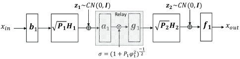
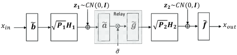
Figure 3: (a) Optimal unquantized scheme for MIMO AF without the direct link, where $\mathbf{H}_{1}=\mathbf{A}\mathbf{\Phi}\mathbf{B}^{H}$ and $\mathbf{H}_{2}=\mathbf{F}\mathbf{\Psi}\mathbf{G}^{H}$. (b) Quantized scheme for MIMO AF without the direct link.

Substituting the optimal solution, found in Theorem 1, in equation (16) reveals the optimal SNR:

$$\gamma^{\star}=\frac{\gamma_{1}^{\star}\gamma_{2}^{\star}}{1+\gamma_{1}^{\star}+\gamma_{2}^{\star}},$$ (21)

where

$$\gamma_{1}^{\star}=\max_{\|\mathbf{s}\|=1}{P_{1}\|\mathbf{H}_{1}\mathbf{s}\|^{2}}=P_{1}\phi_{1}^{2},$$

$$\gamma_{2}^{\star}=\max_{\|\mathbf{s}\|=1}{P_{2}\|\mathbf{H}_{2}\mathbf{s}\|^{2}}=P_{2}\psi_{1}^{2}.$$ (22)

The optimal solution in Theorem 1 verifies the optimality of the scheme in Fig. 3a, where the Tx and relay use the strongest right singular vectors of the Tx-relay and relay-Rx channel matrices for beamforming. Assuming that the relay knows $\mathbf{H}_{1}$ and the receiver knows $\mathbf{H}_{2}$, the optimal structure can be achieved if:

• The relay informs the transmitter of ${\mathbf{b}}_{1}$, the strongest right singular vector of $\mathbf{H}_{1}$.

• The receiver informs the relay of ${\mathbf{g}}_{1}$, the strongest right singular vector of $\mathbf{H}_{2}$.

Considering this, we continue the problem in Subsection III.B by characterizing the codebooks that should be used for quantizing the optimal beamforming vectors.

III-B Quantization Scheme

Fig. 3b presents a scheme which mimics the optimal scheme (Fig. 3a), with the difference that the Tx and relay beamforming vectors belong to certain codebooks with finite cardinality.

In Fig. 3b, the Tx beamforming vector $\tilde{\mathbf{b}}$ should belong to a codebook $\mathbf{C}_{1}(N_{1},\delta_{1})$ shared between the Tx and relay, and similarly, the relay beamforming vector $\tilde{\mathbf{g}}$ should belong to a possibly different codebook $\mathbf{C}_{2}(N_{2},\delta_{2})$, which is shared between the relay and Rx. The relay and Rx use $\tilde{\mathbf{a}}$ and $\tilde{\mathbf{f}}$ for receive beamforming, respectively. All transmit/receive vectors $\tilde{\mathbf{a}}$, $\tilde{\mathbf{b}}$, $\tilde{\mathbf{f}}$ and $\tilde{\mathbf{g}}$ are assumed to be of unit norm, and $\sigma=(1+P_{1}|\tilde{\mathbf{a}}^{H}\mathbf{H}_{1}\tilde{\mathbf{b}}|^{2})^{-1/2}$ in order to satisfy the relay power constraint. The received SNR of the quantized scheme can be easily shown to be equal to:

$$\gamma=\frac{\gamma_{1}\gamma_{2}}{1+\gamma_{1}+\gamma_{2}},$$ (23)

where $\gamma_{1}=P_{1}\left|\tilde{\mathbf{a}}^{H}\mathbf{H}_{1}\tilde{\mathbf{b}}\right|^{2}$ and $\gamma_{2}=P_{2}\left|\tilde{\mathbf{f}}^{H}\mathbf{H}_{2}\tilde{\mathbf{g}}\right|^{2}$ are the received SNRs of the Tx-relay and relay-Rx channels. As $\gamma$ is increasing both in $\gamma_{1}$ and $\gamma_{2}$, we should maximize these quantities to maximize the SNR of the quantized scheme. This is accomplished, as in Section II, by letting $\tilde{\mathbf{a}}$ and $\tilde{\mathbf{f}}$ to be matched to $\mathbf{H}_{1}\tilde{\mathbf{b}}$ and $\mathbf{H}_{2}\tilde{\mathbf{g}}$, and, choosing $\tilde{\mathbf{b}}$ and $\tilde{\mathbf{g}}$ based on: $\tilde{\mathbf{b}}=\arg\max_{\mathbf{w}\in{\mathbf{C}_{1}}}{P_{1}\|\mathbf{H}_{1}{\mathbf{w}}\|^{2}}$ and $\tilde{\mathbf{g}}=\arg\max_{\mathbf{w}\in{\mathbf{C}_{2}}}{P_{2}\|\mathbf{H}_{2}{\mathbf{w}}\|^{2}}$. The corresponding received SNR values are

$$\tilde{\gamma}_{1}=\max_{\mathbf{w}\in{\mathbf{C}_{1}}}{P_{1}\|\mathbf{H}_{1}{\mathbf{w}}\|^{2}},~{}~{}\tilde{\gamma}_{2}=\max_{\mathbf{w}\in{\mathbf{C}_{2}}}{P_{2}\|\mathbf{H}_{2}{\mathbf{w}}\|^{2}},$$ (24)

and the maximum received SNR of the quantized scheme $\tilde{\gamma}$ can be computed by substituting these quantities in (19):

$$\tilde{\gamma}=\frac{\tilde{\gamma}_{1}\tilde{\gamma}_{2}}{1+\tilde{\gamma}_{1}+\tilde{\gamma}_{2}}.$$ (25)

In Appendix II.A, we use the distributions of the optimal beamforming vectors $\mathbf{b}_{1}$ and $\mathbf{g}_{1}$ for Rayleigh channels to compute the following upper bound for the total loss in SNR caused by quantization.

$$\mathrm{E}\{\gamma^{\star}\}-\mathrm{E}\{\tilde{\gamma}\}\leq 2mnP_{1}\left(1{-}N_{1}\left(\frac{\delta_{1}}{2}\right)^{2(m{-}1)}\left(1{-}\frac{\delta_{1}}{2}\right)\right)$$

$$~{}~{}~{}~{}~{}~{}~{}~{}~{}~{}~{}~{}~{}+2nlP_{2}\left(1{-}N_{2}\left(\frac{\delta_{2}}{2}\right)^{2(n{-}1)}\left(1{-}\frac{\delta_{2}}{2}\right)\right),$$ (26)

This upper bound is decreasing in $\delta_{1}$ and $\delta_{2}$ for any $m>1$ and $n>1$. Therefore, to minimize this upper bound, we should maximize the minimum distances $\delta_{1}$ and $\delta_{2}$. This is exactly the criterion used in Grassmannian codebook design and proves the efficiency of these codebooks for quantizing the optimal beamforming vectors. In Section V, we present simulation results which compare the performance of the Grassmannian quantizers with the optimal (unquantized) scheme and other possible quantization schemes.

IV MIMO Amplify and Forward Relay Channel with the Direct Link

In this section the direct link is included in the system model (Fig. 4). The optimal unquantized scheme is derived in Subsection IV.A and the quantization scheme is presented in IV. B. Finally, in IV.C we introduce a modified quantized scheme, which significantly reduces the number of feedback bits with a negligible degradation in the system performance.

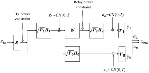
Figure 4: Half-duplex MIMO AF relay channel model with direct link between the transmitter and the receiver.

IV-A Optimal Unquantized Scheme

Consider the half-duplex MIMO-relay link in Fig. 4. At the first time slot, the relay is silent and the Rx receives its symbol. At the second time slot, the Tx is silent and the relay amplifies and forwards its signal (received in the first time slot) to Rx. The receiver has access to two received symbols $y_{0}$ and $y_{1}$ separated in time:

$$y_{0}=\sqrt{P_{0}}\mathbf{r}_{0}^{H}\mathbf{H}_{0}\mathbf{s}x+\mathbf{r}_{0}^{H}\mathbf{z}_{0}$$

$$y_{1}=\sqrt{P_{1}P_{2}}\mathbf{r}_{1}^{H}\mathbf{H}_{2}\mathbf{W}\mathbf{H}_{1}\mathbf{s}x+\mathbf{r}_{1}^{H}\left(\sqrt{P_{2}}\mathbf{H}_{2}\mathbf{W}\mathbf{z}_{1}+\mathbf{z}_{2}\right).$$

The receiver computes the linear MMSE combination of $y_{0}$ and $y_{1}$ to compute the output symbol $x_{out}$:

$$x_{out}=\alpha_{0}y_{0}+\alpha_{1}y_{1}.$$

By proper choice of $\alpha_{0}$ and $\alpha_{1}$ the output SNR is:

$$\gamma=\gamma_{0}+\gamma_{r},$$ (27)

where $\gamma_{0}$ and $\gamma_{r}$ are the received SNR values of the direct link and the Tx-relay-Rx link. Therefore, the total SNR is maximized if the received SNRs of the direct and relay links are maximized. The only common parameter in maximizing these two quantities is the Tx beamforming vector $\mathbf{s}$.

By fixing $\mathbf{s}$ and following the same steps in Sections II and III, the optimal values of other parameters can be easily derived, as showed in Fig. 5a. In the first time slot, the relay and the Rx should respectively match to $\mathbf{H}_{1}\mathbf{s}$ and $\mathbf{H}_{0}\mathbf{s}$ at their inputs. In the second time slot, the relay maps its normalized symbol to $\mathbf{g}_{1}$ the strongest right singular vector of $\mathbf{H}_{2}$ and the receiver uses $\mathbf{f}_{1}$, the strongest left singular vector of $\mathbf{H}_{2}$, for receive beamforming. The corresponding received SNRs of the direct link and relay link are:

$$\gamma_{0}=P_{0}\|\mathbf{H}_{0}\mathbf{s}\|^{2}$$

$$\gamma_{r}=\frac{\gamma_{1}\gamma_{2}^{\star}}{1+\gamma_{1}+\gamma_{2}^{\star}},$$ (28)

where $\gamma_{1}=P_{1}\|\mathbf{H}_{1}\mathbf{s}\|^{2}$ and $\gamma_{2}^{\star}$ is the maximum received SNR of the the relay-Rx link: $\gamma_{2}^{\star}=P_{2}\|\mathbf{H}_{2}\mathbf{g}_{1}\|^{2}=P_{2}\psi_{1}^{2}$. By combining (23) and (24) the total received SNR is:

$$\gamma=\frac{P_{1}\|\mathbf{H}_{1}\mathbf{s}\|^{2}\gamma_{2}^{\star}}{1+P_{1}\|\mathbf{H}_{1}\mathbf{s}\|^{2}+\gamma_{2}^{\star}}+P_{0}\|\mathbf{H}_{0}\mathbf{s}\|^{2},$$

and therefore, the optimal $\mathbf{s}$ can be expressed as:

$$\mathbf{s}^{\star}=\arg\max_{\|\mathbf{s}\|=1}{\frac{\|\mathbf{H}_{1}\mathbf{s}\|^{2}}{\|\mathbf{H}_{1}\mathbf{s}\|^{2}+\lambda}+\mu\|\mathbf{H}_{0}\mathbf{s}\|^{2}},$$ (29)

where $\lambda=\frac{1+\gamma_{2}^{\star}}{P_{1}}$ and $\mu=\frac{P_{0}}{\gamma_{2}^{\star}}$. The corresponding total received SNR is:

$$\gamma^{\star}=\frac{\gamma_{1}^{\star}\gamma_{2}^{\star}}{1+\gamma_{1}^{\star}+\gamma_{2}^{\star}}+\gamma_{0}^{\star},$$ (30)

where $\gamma_{0}^{\star}=P_{0}\|\mathbf{H}_{0}\mathbf{s}^{\star}\|^{2}$ and $\gamma_{1}^{\star}=P_{1}\|\mathbf{H}_{1}\mathbf{s}^{\star}\|^{2}$.

The objective function of the problem in (25) has multiple local maximum points and moreover, the global maximum point is not unique. This problem does not appear to have an analytic solution and as a result we use a numerical approach to perform this optimization, which will be described in Section V.

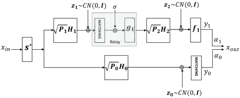
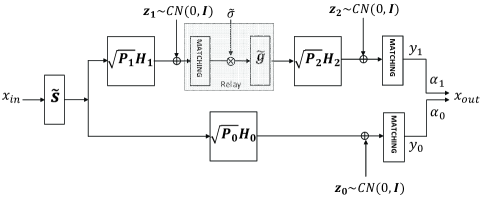
Figure 5: (a) Optimal unquantized scheme for MIMO AF with the direct channel. In the first time slot, the relay and the Rx match to $\mathbf{H}_{1}\mathbf{s}^{\star}$ and $\mathbf{H}_{0}\mathbf{s}^{\star}$, respectively. (b) Quantized scheme for MIMO AF with direct link. In the first time slot, the relay and the Rx match to $\mathbf{H}_{1}\tilde{\mathbf{s}}$ and $\mathbf{H}_{0}\tilde{\mathbf{s}}$, respectively. In the second time slot, the relay matches to $\mathbf{H}_{2}\tilde{\mathbf{g}}$. When $\tilde{\mathbf{s}}$ is replaced by $\tilde{\mathbf{s}}^{\star}$ in (31), we will refer to this system as the “properly quantized scheme”.

Despite the fact that we do not have a closed form expression for the solution of problem (25), we are still able to identify the distribution of the solution for Rayleigh fading channels. The main result of this section is the following theorem.

Theorem 2

For independent Rayleigh channel matrices $\mathbf{H}_{0}$ and $\mathbf{H}_{1}$, the optimal Tx beamforming vector $\mathbf{s}^{\star}$ that maximizes the total received SNR (or equivalently the objective function in (25)) is uniformly distributed on the unit sphere in $\mathds{C}^{m}$, where $m$ is the number of Tx antennas.

Proof:

See Appendix I. ∎

Note that if we had a single channel from the transmitter to the receiver, the optimal Tx beamforming vector would be uniformly distributed on the unit sphere in $\mathds{C}^{m}$ (see Section II). Interestingly, Theorem 2 states that the optimal Tx beamforming vector is still uniformly distributed on the unit sphere, when there are two independent parallel channels from the transmitter to the receiver. This is basically due to the independence of $\mathbf{H}_{0}$ and $\mathbf{H}_{1}$, and the specific properties of the Rayleigh channel matrices.

The result in Theorem 2 is used in Appendix II.B to derive an SNR loss upper bound, similar to (2) and (22), which justifies use of the Grassmannian codebook for quantizing the optimal Tx beamforming vector $\mathbf{s}^{\star}$.

IV-B Quantization Scheme

Having identified the optimal scheme, we continue by considering the quantization scheme in Fig. 5b. In the first time slot, the Tx uses $\tilde{\mathbf{s}}$ for beamforming, and relay and Rx match their receive vectors to $\mathbf{H}_{1}\tilde{\mathbf{s}}$ and $\mathbf{H}_{0}\tilde{\mathbf{s}}$. In the second time slot, the relay scales its symbol and uses $\tilde{\mathbf{g}}$ for beamforming and Rx matches to $\mathbf{H}_{2}\tilde{\mathbf{g}}$. The Tx-Rx, Tx-relay, relay-Rx and total received SNR values is given by:

$${\gamma}_{0}=P_{0}\|\mathbf{H}_{0}\tilde{\mathbf{s}}\|^{2},~{}~{}{\gamma}_{1}=P_{1}\|\mathbf{H}_{1}\tilde{\mathbf{s}}\|^{2},~{}~{}{\gamma}_{2}=P_{2}\|\mathbf{H}_{2}\tilde{\mathbf{g}}\|^{2}$$

$$\gamma=\frac{\gamma_{1}\gamma_{2}}{1+\gamma_{1}+\gamma_{2}}+{\gamma}_{0}.$$ (31)

We need to maximize (27) with respect to the Tx and relay beamforming vectors $\tilde{\mathbf{s}}$ and $\tilde{\mathbf{g}}$, which belong to certain codebooks with finite cardinalities. As in Section III, we assume that the codebooks $\mathbf{C}_{1}(N_{1},\delta_{1})$ and $\mathbf{C}_{2}(N_{2},\delta_{2})$ are shared between Tx-relay and relay-Rx, respectively. Clearly, $\tilde{\mathbf{g}}$ should be chosen to maximize ${\gamma}_{2}$:

$$\tilde{\mathbf{g}}=\arg\max_{\mathbf{w}\in\mathbf{C}_{2}}{P_{2}\|\mathbf{H}_{2}{\mathbf{w}}\|^{2}}.$$ (32)

The corresponding relay-Rx received SNR is: $\tilde{\gamma}_{2}=\max_{\mathbf{w}\in\mathbf{C}_{2}}{P_{2}\|\mathbf{H}_{2}{\mathbf{w}}\|^{2}}$.

For choosing the proper $\tilde{\mathbf{s}}$, we need to know both $\mathbf{H}_{0}$ and $\mathbf{H}_{1}$. We continue the problem here by assuming that the relay knows $\mathbf{H}_{0}$ in addition to its channel $\mathbf{H}_{1}$. This assumption will be relaxed in IV.B.2.

IV-B1 Complete Knowledge of $\mathbf{H}_{0}$ at the Relay

If the relay knows both $\mathbf{H}_{0}$ and $\mathbf{H}_{1}$, then based on (27) the best vector $\tilde{\mathbf{s}}$ should be chosen as follows:

$$\tilde{\mathbf{s}}=\arg\max_{\mathbf{w}\in\mathbf{C}_{1}}{\frac{\|\mathbf{H}_{1}\mathbf{w}\|^{2}}{\|\mathbf{H}_{1}\mathbf{w}\|^{2}+\tilde{\lambda}}+\tilde{\mu}\|\mathbf{H}_{0}\mathbf{w}\|^{2}},$$ (33)

where $\tilde{\lambda}=\frac{1+\tilde{\gamma}_{2}}{P_{1}}$ and $\tilde{\mu}=\frac{P_{0}}{\tilde{\gamma}_{2}}$. The maximum total received SNR of the quantized scheme $\tilde{\gamma}$ can be computed by substituting (28) and (29) in (27).

In Appendix II.B, we use the distribution of $\mathbf{s}^{\star}$, given in Theorem 2, to prove the following bound on the SNR loss caused by quantization.

$$\mathrm{E}\{\gamma^{\star}\}-\mathrm{E}\{\tilde{\gamma}\}$$

$$~{}~{}~{}\leq 2\left(mlP_{0}+mnP_{1}\right)\left(1{-}N_{1}\left(\frac{\delta_{1}}{2}\right)^{2(m{-}1)}\left(1{-}\frac{\delta_{1}}{2}\right)\right)$$

$$~{}~{}~{}~{}~{}~{}~{}~{}~{}~{}~{}~{}+2nlP_{2}\left(1{-}N_{2}\left(\frac{\delta_{2}}{2}\right)^{2(n{-}1)}\left(1{-}\frac{\delta_{2}}{2}\right)\right).$$ (34)

This upper bound is decreasing in $\delta_{1}=\delta(\mathbf{C}_{1})$ and $\delta_{2}=\delta(\mathbf{C}_{2})$ for any $m,n>1$ and justifies the use of Grassmannian codebooks, $\mathbf{C}_{1}$ and $\mathbf{C}_{2}$, for quantizing the optimal Tx and relay beamforming vectors, $\mathbf{s}^{\star}$ and $\mathbf{g}_{1}$.

IV-B2 Partial Knowledge of $\mathbf{H}_{0}$ at the Relay

As mentioned earlier, the computations in IV.B.1 are based on the assumption that the relay knows $\mathbf{H}_{0}$ completely. In reality, however, the Rx needs to quantize $\mathbf{H}_{0}$ and send it to the relay. We should note that, the only way that $\mathbf{H}_{0}$ contributes to the problem in (28) is through the term $\|\mathbf{H}_{0}\mathbf{w}\|^{2}$, which can be expanded as follows: $\|\mathbf{H}_{0}\mathbf{w}\|^{2}=\sum_{i=1}^{R_{0}}{\nu_{i}^{2}|\mathbf{e}_{i}^{H}\mathbf{w}|^{2}}$, where $\nu_{i}$’s and $\mathbf{e}_{i}$’s are the singular values and right singular vectors of $\mathbf{H}_{0}$ and $R_{0}=\texttt{rank}({\mathbf{H}_{0}})$. Therefore, the relay only needs to know the singular values and the right singular vectors of the direct link channel. Since our focus in this paper is on the vector quantization feedback schemes, we assume that the relay knows the singular values completely but has only access to the quantized versions of the singular vectors.

For quantizing the singular vectors, the Rx and the relay share a codebook $\mathbf{C}_{0}(N_{0},\delta_{0})$, which is possibly different from $\mathbf{C}_{2}$ (used for determining $\tilde{\mathbf{g}}$). We assume that the Rx quantizes each vector $\mathbf{e}_{i}$ to a vector $\tilde{\mathbf{e}}_{i}\in\mathbf{C}_{0}$ that is closest to $\mathbf{e}_{i}$.

$$\tilde{\mathbf{e}}_{i}=\arg\min_{\mathbf{w}\in\mathbf{C}_{0}}{d(\mathbf{w},\mathbf{e}_{i})}.$$

Having $\nu_{i}$’s and $\tilde{\mathbf{e}}_{i}$’s at the relay, the problem of finding the Tx beamforming vector $\tilde{\mathbf{s}}^{\star}$ can be reformulated as:

$$\tilde{\mathbf{s}}^{\star}=\arg\max_{\mathbf{w}\in\mathbf{C}_{1}}{\frac{\|\mathbf{H}_{1}\mathbf{w}\|^{2}}{\|\mathbf{H}_{1}\mathbf{w}\|^{2}+\tilde{\lambda}}+\tilde{\mu}{\sum_{i=1}^{R_{0}}{\nu_{i}^{2}|\tilde{\mathbf{e}}_{i}^{H}\mathbf{w}|^{2}}},}$$ (35)

where $\tilde{\lambda}=\frac{1+\tilde{\gamma}_{2}}{P_{1}}$, $\tilde{\mu}=\frac{P_{0}}{\tilde{\gamma}_{2}}$, and $\tilde{\gamma}_{2}=\max_{\mathbf{w}\in\mathbf{C}_{2}}{P_{2}\|\mathbf{H}_{2}{\mathbf{w}}\|^{2}}$. The total received SNR $\tilde{\gamma}^{\star}$ can be computed by substituting (28) and (31) in (27). Finally, the loss in the received SNR can be bounded as follows (see Appendix II.C).

$$\mathrm{E}\{\gamma^{\star}\}-\mathrm{E}\{\tilde{\gamma}^{\star}\}$$

$$~{}\leq 2\left(mlP_{0}+mnP_{1}\right)\left(1{-}N_{1}\left(\frac{\delta_{1}}{2}\right)^{2(m{-}1)}\left(1{-}\frac{\delta_{1}}{2}\right)\right)$$

$$~{}~{}~{}~{}~{}~{}~{}~{}~{}~{}+2nlP_{2}\left(1{-}N_{2}\left(\frac{\delta_{2}}{2}\right)^{2(n{-}1)}\left(1{-}\frac{\delta_{2}}{2}\right)\right)$$

$$~{}~{}~{}~{}~{}~{}~{}~{}~{}~{}+4mlP_{0}\left(1{-}N_{0}\left(\frac{\delta_{0}}{2}\right)^{2(m{-}1)}\left(1{-}\frac{\delta_{0}}{2}\right)\right).$$ (36)

The upper bound in (32) is decreasing in $\delta_{0}=\delta(\mathbf{C}_{0})$ for any $m>1$. This justifies use of the Grassmannian codebook to quantize the singular vectors of $\mathbf{H}_{0}$, since it has the maximum minimum distance $\delta_{0}$. The same conclusion holds for $\mathbf{C}_{1}$ and $\mathbf{C}_{2}$, since the upper bound in (32) is decreasing in $\delta_{1}$ and $\delta_{2}$ for any $m,n>1$.

To summarize the results, all three codebooks $\mathbf{C}_{0}$, $\mathbf{C}_{1}$ and $\mathbf{C}_{2}$ need to be Grassmannian codebooks to minimize the upper bound of the loss in the total received SNR. We refer to the scheme, determined by (31), as the “properly quantized scheme”. In the following we outline the steps in determining the beamforming vectors of the “properly quantized scheme” (Fig. 5b).

1. The Rx uses a Grassmannian codebook $\mathbf{C}_{2}$, shared between the Rx and the relay, to quantize $\mathbf{g}$, the strongest right singular vector of the relay-Rx channel $\mathbf{H}_{2}$. The label of the quantized vector is sent to the relay. The relay uses this vector for its beamforming in the second time slot. The Rx also sends the SNR value $\tilde{\gamma}_{2}$ to the relay. This will be used in step 3.

2. The Rx quantizes the right singular vectors of the Tx-Rx channel using a Grassmannian codebook $\mathbf{C}_{0}$, which is shared between the Rx and the relay. The labels of the quantized vectors and the singular values $\nu_{i}$’s are sent to the relay.

3. The relay forms the objective function in (31) and maximizes it over the Grassmannian codebook $\mathbf{C}_{1}$, which is shared between the Tx and the relay. The relay sends the label of the maximizing vector to the Tx. The transmitter uses this vector for its beamforming in the first time slot.

Before concluding Section IV, we introduce a modified scheme which performs very close to the “properly quantized scheme” but requires fewer number of feedback bits.

IV-C Modified Quantized Scheme

Consider the problem of determining the Tx beamforming vector for the quantized scheme in Fig. 5b (see equation (31)). There are two links between the transmitter and the receiver; the direct (Tx-Rx) link and the Tx-relay-Rx link, which we refer to as the relay link. If the direct link is much weaker than the relay link and can be ignored safely, our problem reduces to the problem in Section III and the relay does not need to know anything about the direct link channel $\mathbf{H}_{0}$. On the other hand, if the relay link is very weak and can be ignored, the only thing that we need to know about $\mathbf{H}_{0}$ is its strongest right singular vector. Therefore, in both of these extreme cases we do not need to have any knowledge of $\mathbf{H}_{0}$ other than its strongest right singular vector. Based on this intuition, we propose a new scheme, referred to as the “modified quantized scheme”, in which the Rx only quantizes the strongest right singular vector of $\mathbf{H}_{0}$ and sends the corresponding label (and the largest singular value $\nu_{1}$) to the relay. The relay then determines the proper Tx beamforming vector by forming the following problem.

$$\tilde{\mathbf{s}}_{modified}=\arg\max_{\mathbf{w}\in\mathbf{C}_{1}}{\frac{\|\mathbf{H}_{1}\mathbf{w}\|^{2}}{\|\mathbf{H}_{1}\mathbf{w}\|^{2}+\tilde{\lambda}}+\tilde{\mu}\nu_{1}^{2}|\tilde{\mathbf{e}}_{1}^{H}\mathbf{w}|^{2}},$$ (37)

where $\tilde{\lambda}$ and $\tilde{\mu}$ have the same definitions as in (31).

The “modified quantized scheme” requires much fewer number of bits, since it only quantizes one singular vector (see step 2 for the properly quantized scheme). Our simulation results show that the “modified quantized scheme” performs very close to the “properly quantized scheme”, as we will see in Section V.

V Simulation Results

In this section, we provide simulation results for the scenarios discussed in the Sections III and IV. The results are divided into two subsections. In V.A the direct link between the transmitter and the receiver is ignored, as in Section III (see Fig. 2). In V.B, the simulation results are presented for the case where the direct link is present in the model (Fig. 4).

The general setup for the simulations is as follows. The input symbols belong to a BPSK constellation with unit power. The entries of the channel matrices, which model the i.i.d Rayleigh fading channels, are generated independently according to $\mathcal{CN}(0,1)$. To model quasi-static fading channels, the simulation time is divided to $20,000$ coherence intervals, each consisting of $200$ symbols. The channels are assumed to be constant over each coherence interval and to be independent from one interval to the other. The simulation results compare different (quantized and unquantized) schemes from the bit-error-rate (BER) point of view.

V-A MIMO AF Relay Channel without the Direct Link

In this section, the direct link is not considered in the simulation model (Fig. 2). All of the stations (Tx, relay and Rx) are assumed to have two antennas ($m=n=l=2$). The relay-Rx link SNR is fixed at $P_{2}=8$dB and the BER values have been recorded for different values of the Tx-relay link SNR $P_{1}$. For the quantization purposes, the Tx and relay share a codebook $\mathbf{C}_{1}$ of size $N_{1}$. Similarly, the relay and Rx share a codebook $\mathbf{C}_{2}$ of size $N_{2}$.

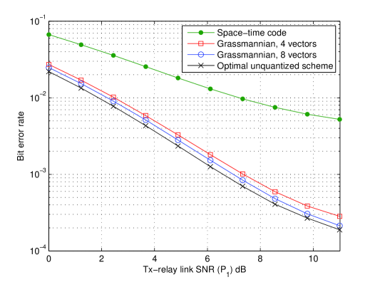
Figure 6: Comparison of the performance of Grassmannian quantization scheme with the optimal (unquantized) scheme and the Alamouti space-time coding. The relay-Rx link SNR is fixed at $8$dB.

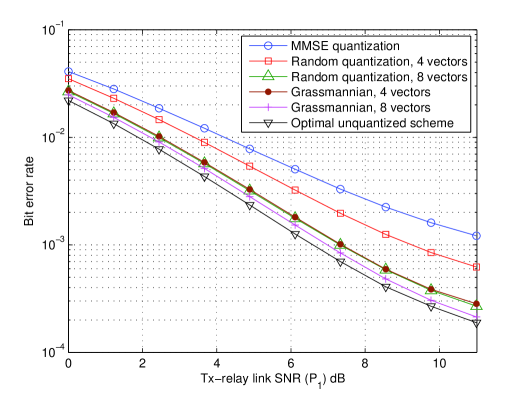
Figure 7: Comparison of the performance of the Grassmannian quantizer with the MMSE and random quantizers. The relay-Rx link SNR is fixed at $8$dB.

Fig. 6 compares the performance of the “optimal unquantized scheme” (Fig. 3a) with the performance of the Grassmannian codebooks $\mathbf{C}_{1}$ and $\mathbf{C}_{2}$ of sizes $N_{1}=N_{2}=4$ or $8$. The Grassmannian codebooks are adopted from [5]. The total number of the feedback bits used by the Grassmannian quantizer is $\log_{2}{N_{1}}+\log_{2}{N_{2}}$ which equals $4$ or $6$ bits for $N_{1}=N_{2}=4$ or $8$. As Fig. 6 shows, we can get very close to the optimal scheme with only a few number of bits per each coherence interval. We have also simulated the performance of the Alamouti code, to show the high power gain that can be achieved by using the Grassmannian codebooks compared to space-time codes.

In Fig. 7 we compare the performance of the Grassmannian quantizers with other quantization schemes. For the MMSE quantization scheme, the Rx and relay quantize every entry of the channel matrices $\mathbf{H}_{2}$ and $\mathbf{H}_{1}$ according to the MMSE criterion and send the quantized channel matrices to the relay and Tx, respectively. The Tx and the relay perform singular value decomposition on these quantized matrices and use the corresponding strongest right singular vectors for beamforming. We have assumed that the quantizer uses two bits to quantize each channel entry, i.e., one bit for each of the real and imaginary parts. For $m=n=l=2$ this results in $2(mn+nl)=16$ bits which should be compared to the small number of feedback bits in the Grassmannian scheme.

Fig. 7 also compares the Grassmannian quantizer with the random quantization scheme. The random quantizer uses a set of randomly selected vectors on the unit sphere as its quantization codebook. The performance of the random scheme has been averaged over ten such codebooks. As Fig. 7 shows, the Grassmannian scheme shows considerable gain as compared with the random quantizer. However, this gain decreases as the codebook sizes are increased from $4$ to $8$. The main advantage of the random codebooks is that they are easy to generate as compared with the Grassmannian codebooks.

V-B MIMO AF Relay Channel with the Direct Link

In this section, we simulate the system model in Section IV, where the direct link has been included in the analysis. All the stations are equipped with three antennas ($m=n=l=3$).

Fig. 8 compares the “optimal unquantized scheme” (Fig. 5a) with some other unquantized schemes. The Tx-relay and relay-Rx link SNR’s are fixed at $P_{1}=P_{2}=2$dB and the BER values are recorded for different values of the direct link SNR $P_{0}$. For the optimal scheme, we use the gradient descent method for determining the Tx beamforming vector from (25). The constraint $\|\mathbf{s}\|=1$ is eliminated by the change of variable $\mathbf{s}=\frac{\mathbf{u}}{\|\mathbf{u}\|}$.

The curve marked by $\triangledown$ shows the performance of the scheme that ignores the direct link in determining the Tx beamforming vector. For this scheme, the Tx beamforming vector is always set to the strongest right singular vector of the Tx-relay channel. As expected, the performance of this scheme diverges from the optimal scheme as the direct link gets stronger. The next curve, marked by $\square$, shows the performance of the scheme which considers only the stronger link for determining the Tx beamforming vector. In this scheme, the Tx switches between the strongest right singular vectors of the Tx-relay and Tx-Rx links depending on their received SNR values. The last scheme, called the “modified unquantized scheme”, has the same structure as the “optimal unquantized scheme” with the difference that the relay only considers the strongest singular value and singular vector of $\mathbf{H}_{0}$ in formulating the problem of determining the Tx beamforming vector. This problem is exactly the same as the problem (25), used by the optimal scheme, except that $\|\mathbf{H}_{0}\mathbf{s}\|^{2}$ is replaced by $\nu_{1}^{2}|\mathbf{e}_{1}^{H}\mathbf{s}|^{2}$, where $\nu_{1}$ and $\mathbf{e}_{1}$ are the strongest singular value and right singular vector of $\mathbf{H}_{0}$. In Appendix III, we show that the average SNR loss of this scheme with respect to the optimal scheme is at most $1.24$dB for the system with $m=n=l=3$ antennas. As the simulation results in Fig. 8 verify, the modified unquantized scheme performs very close to the optimal scheme. This unquantized scheme is the basis for a quantization scheme that has been referred to as the “modified quantized scheme” in Section IV (see (33)).

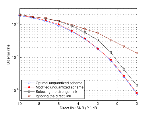
Figure 8: Comparison of the optimal unquantized scheme with other unquantized schemes. The Tx-relay and relay-Rx link SNRs are fixed at $P_{1}=P_{2}=2$dB.

In the next two simulation setups, we study the performance of the quantized schemes. As discussed in Section IV, the scheme consists of three codebooks $\mathbf{C}_{0}$, $\mathbf{C}_{1}$ and $\mathbf{C}_{2}$ of sizes $N_{0}$, $N_{1}$ and $N_{2}$. The codebook $\mathbf{C}_{0}$ is used for quantization of the direct link channel $\mathbf{H}_{0}$. The codebook $\mathbf{C}_{2}$ is used to determine the relay beamforming vector in the second time slot. The codebook $\mathbf{C}_{1}$ determines the Tx beamforming vector in the first time slot. Fig. 9 shows the performance of the “properly quantized scheme” with Grassmannian codebooks of sizes $N_{1}=N_{2}=N_{3}=8,16$ (see the three steps for properly quantized scheme in Section IV). The Tx-relay and relay-Rx link SNRs are fixed at $P_{1}=P_{2}=2$dB and the BER values have been recorded for different values of the direct link SNR $P_{0}$. The Grassmannian codebooks are adopted from [14].

The figure also shows the performance of the Grassmannian codebooks with “modified quantized scheme” (see (33)). This scheme shows a negligible performance degradation with respect to the “properly quantized scheme”, but requires fewer number of feedback bits. As an example, we compare the total number of bits required by the properly quantized and the modified quantized scheme. For quantization of the scalar values, we assume a hypothetical quantizer which requires $b$ bits for quantizing a scalar quantity. Recall the three steps of the properly quantized scheme in Section IV. For step one, we need $\log_{2}(N_{2})$ bits for quantizing $\mathbf{g}$ and $b$ bits for quantizing $\tilde{\gamma}_{2}$. In step two, we need $R_{0}(\log_{2}(N_{0})+b)$ for the “properly quantized scheme” and $\log_{2}(N_{0})+b$ bits for the “modified quantized scheme”, where $R_{0}=\texttt{rank}(\mathbf{H}_{0})$. Finally, for the third step, we need $\log_{2}(N_{1})$ bits for quantizing the Tx beamforming vector. Therefore, we need a total of $(1+R_{0})b+\log_{2}(N_{0}^{R_{0}}N_{1}N_{2})$ bits for the “properly quantized scheme” and $2b+\log_{2}(N_{0}N_{1}N_{2})$ bits for the “modified quantized scheme”. Table I compares these values for $N=N_{0}=N_{1}=N_{2}=8,~{}16$, and $m=n=l=3$. Here we have assumed a full rank channel matrix $\mathbf{H}_{0}$.

TABLE I: Comparison of the Number of the Feedback Bits for Different Quantization Schemes

Scheme	Number of feedback bits
	$~{}~{}N=8~{}~{}$	$N{=}16$
Properly quantized	$15+4b$	$20+4b$
Modified quantized	$9+2b$	$12+2b$
MMSE	$54+b$

Fig. 9 also shows the performance of the MMSE quantizer. This quantizer requires $2(mn+ml+ln)$ bits for quantizing the channel matrices and $b$ bits for quantizing $\tilde{\gamma}_{2}$.

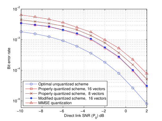
Figure 9: Comparison of the properly quantized scheme with modified quantized and MMSE quantization schemes. The Tx-relay and relay-Rx link SNRs are fixed at $P_{1}=P_{2}=2$dB.

Fig. 10 compares the performance of the same schemes of Fig. 9 in a different scenario. For this figure, the direct link and relay-Rx link SNR are fixed at $P_{0}=-4$dB and $P_{2}=2$dB. The BER values have been recorded for different values of the Tx-relay link SNR $P_{1}$. Once again, we see that the performance of the “modified quantized scheme” is very close to the “properly quantized scheme”.

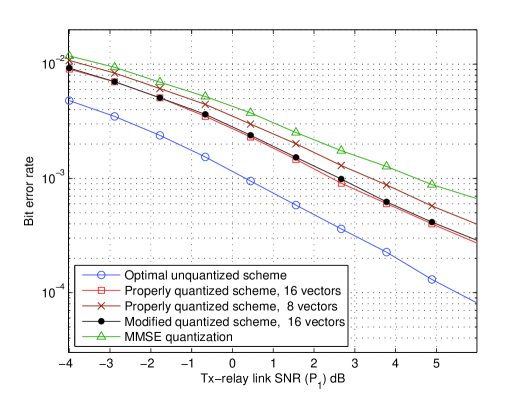
Figure 10: Comparison of the properly quantized scheme with modified quantized and MMSE quantization schemes. The direct link and relay-Rx link SNR are fixed at $P_{0}=-4$dB and $P_{2}=2$dB.

VI Conclusion

In this paper, we derived the optimal (unquantized) Tx/Rx beamforming vectors and the optimal relay weighting matrix to maximize the total received SNR of MIMO AF relay channel both with and without the direct Tx-Rx link. We showed that the Grassmannian codebooks are appropriate choices for the quantization codebooks in the quantized scheme. We proposed a modified quantized scheme which performs very close to this quantized scheme and requires considerably fewer number of feedback bits. Finally, the analytical results were verified by comparing the performance of the unquantized and quantized schemes under different scenarios.

Appendix A The Distribution of the Optimal Beamforming Vector $\mathbf{s}^{\star}$

In this appendix, we show that there exists a solution $\mathbf{s}^{\star}$ to the problem (25) that is uniformly distributed on the unit sphere in $\mathds{C}^{m}$, where $m$ is the number of Tx antennas.

The problem (25) is repeated here:

$$\mathbf{s}^{\star}=\arg\max_{\|\mathbf{s}\|=1}{\frac{\|\mathbf{H}_{1}\mathbf{s}\|^{2}}{\|\mathbf{H}_{1}\mathbf{s}\|^{2}+\lambda}+\mu\|\mathbf{H}_{0}\mathbf{s}\|^{2}},$$ (A.1)

Consider $\mathbf{H}_{0}=\mathbf{U}_{0}\mathbf{\Sigma}_{0}\mathbf{V}_{0}^{H}$ and $\mathbf{H}_{1}=\mathbf{U}_{1}\mathbf{\Sigma}_{1}\mathbf{V}_{1}^{H}$ as the SVD of $\mathbf{H}_{0}$ and $\mathbf{H}_{1}$. Clearly: $\|\mathbf{H}_{0}\mathbf{s}\|=\left\|\mathbf{\Sigma}_{0}\mathbf{V}_{0}^{H}\mathbf{s}\right\|$ and $\left\|\mathbf{H}_{1}\mathbf{s}\right\|=\left\|\mathbf{\Sigma}_{1}\mathbf{V}_{1}^{H}\mathbf{s}\right\|$, since $\mathbf{U}_{0}$ and $\mathbf{U}_{1}$ are unitary matrices.

It is easy to check that $\mathbf{s}^{\star}=\mathbf{V}_{0}\eta(\mathbf{\Sigma}_{0},\mathbf{\Sigma}_{1},\mathbf{V}_{1}^{H}\mathbf{V}_{0})$ is a solution to (I.1), where the function $\eta(\cdot,\cdot,\cdot)$ is defined to be a solution to the following problem:

$$\eta(\mathbf{\Sigma}_{0}, \mathbf{\Sigma}_{1} ,\mathbf{V}_{1}^{H}\mathbf{V}_{0})$$ (A.2)

$$\stackrel{{\scriptstyle def}}{{=}} \arg\max_{\|\mathbf{t}\|=1}{\frac{\left\|\mathbf{\Sigma}_{1}\mathbf{V}_{1}^{H}\mathbf{V}_{0}\mathbf{t}\right\|^{2}}{\left\|\mathbf{\Sigma}_{1}\mathbf{V}_{1}^{H}\mathbf{V}_{0}\mathbf{t}\right\|^{2}+\lambda}+\mu\left\|\mathbf{\Sigma}_{0}\mathbf{t}\right\|^{2}}.$$

If we fix $\mathbf{\Sigma}_{0}$ and $\mathbf{\Sigma}_{1}$, the solution $\mathbf{s}^{\star}$, identified above, can be expressed as a function of $\mathbf{V}_{0}$ and $\mathbf{V}_{1}$:

$$\mathbf{s}^{\star}=\zeta_{{}_{\mathbf{\Sigma}_{0},\mathbf{\Sigma}_{1}}}(\mathbf{V}_{0},\mathbf{V}_{1})\stackrel{{\scriptstyle def}}{{=}}\mathbf{V}_{0}\eta(\mathbf{\Sigma}_{0},\mathbf{\Sigma}_{1},\mathbf{V}_{1}^{H}\mathbf{V}_{0}).$$ (A.3)

Now, for any unitary matrix $\mathbf{Q}$, we have the following from (I.3).

$$\zeta_{{}_{\mathbf{\Sigma}_{0},\mathbf{\Sigma}_{1}}}(\mathbf{Q}\mathbf{V}_{0},\mathbf{Q}\mathbf{V}_{1})=\mathbf{Q}\zeta_{{}_{\mathbf{\Sigma}_{0},\mathbf{\Sigma}_{1}}}(\mathbf{V}_{0},\mathbf{V}_{1})=\mathbf{Q}\mathbf{s}^{\star}.$$

For a Rayleigh channel matrix $\mathbf{H}_{0}$, we know the the random matrix $\mathbf{V}_{0}$ is independent of $\mathbf{\Sigma}_{0}$ and its distribution does not change by pre-multiplication by a unitary matrix $\mathbf{Q}$. The same argument holds for $\mathbf{H}_{1}$, $\mathbf{V}_{1}$ and $\mathbf{\Sigma}_{1}$. Therefore, conditioned on $\mathbf{\Sigma}_{0}$ and $\mathbf{\Sigma}_{1}$, the matrix $\mathbf{Q}\mathbf{V}_{0}$ has the same distribution as $\mathbf{V}_{0}$, and similarly $\mathbf{Q}\mathbf{V}_{1}$ has the same distribution as $\mathbf{V}_{1}$. Since the Tx-Rx and Tx-relay channels are assumed to be independent, $\mathbf{V}_{0}$ and $\mathbf{V}_{1}$ are also independent, and therefore the joint distribution of $(\mathbf{V}_{0},\mathbf{V}_{1})$ is also the same as the joint distribution of $(\mathbf{Q}\mathbf{V}_{0},\mathbf{Q}\mathbf{V}_{1})$. Hence, any arbitrary function of these pairs will have the same distribution. By applying this to the function $\zeta_{{}_{\mathbf{\Sigma}_{0},\mathbf{\Sigma}_{1}}}(\cdot)$, we conclude that $\mathbf{s}^{\star}=\zeta_{{}_{\mathbf{\Sigma}_{0},\mathbf{\Sigma}_{1}}}(\mathbf{V}_{0},\mathbf{V}_{1})$ and $\mathbf{Q}\mathbf{s}^{\star}=\zeta_{{}_{\mathbf{\Sigma}_{0},\mathbf{\Sigma}_{1}}}(\mathbf{Q}\mathbf{V}_{0},\mathbf{Q}\mathbf{V}_{1})$ have the same distribution. Since this it true for any unitary matrix $\mathbf{Q}$, we conclude that $\mathbf{s}^{\star}$ is uniformly distributed on the complex unit sphere, conditioned on $\mathbf{\Sigma}_{0}$ and $\mathbf{\Sigma}_{1}$.

Note that if the conditional distribution of $\mathbf{s}^{\star}$ is uniform, its unconditional distribution is also uniform. Moreover, the random vector $\mathbf{s}^{\star}$ is independent of the random matrices $\mathbf{\Sigma}_{0}$ and $\mathbf{\Sigma}_{1}$, since its conditional and unconditional distributions are the same.

Appendix B Proof of SNR Loss Upper Bounds

In this appendix, we prove the SNR loss upper bounds of (22), (30) and (32) in three separate sections. We will first prove the following lemmas, which are frequently used in these sections.

Lemma 1

For nonnegative variables $x_{1}$, $x_{2}$, $y_{1}$ and $y_{2}$, we have:

$$\left|\frac{x_{1}y_{1}}{1+x_{1}+y_{1}}-\frac{x_{2}y_{2}}{1+x_{2}+y_{2}}\right|\leq|x_{1}-x_{2}|+|y_{1}-y_{2}|.$$

Proof:

We use the following inequality, which can be easily verified by basic computations. For any $a\geq 0$, $b\geq 0$ and $c>0$ we have:

$$\left|\frac{a}{a+c}-\frac{b}{b+c}\right|\leq\frac{1}{c}|a-b|.$$ (B.1)

Now the expression in Lemma 1 can be written as:

$$~{}\left|\frac{x_{1}y_{1}}{1{+}x_{1}{+}y_{1}}-\frac{x_{2}y_{2}}{1{+}x_{2}{+}y_{2}}\right|$$

$${\stackrel{{\scriptstyle\textmd{(a)}}}{{{\leq}}}}\left|\frac{x_{1}y_{1}}{1{+}x_{1}{+}y_{1}}{-}\frac{x_{1}y_{2}}{1{+}x_{1}{+}y_{2}}\right|{+}\left|\frac{x_{1}y_{2}}{1{+}x_{1}{+}y_{2}}{-}\frac{x_{2}y_{2}}{1{+}x_{2}{+}y_{2}}\right|$$

$$=x_{1}\left|\frac{y_{1}}{y_{1}{+}{(}x_{1}{+}1{)}}{-}\frac{y_{2}}{y_{2}{+}{(}x_{1}{+}1{)}}\right|{+}y_{2}\left|\frac{x_{1}}{x_{1}{+}{(}y_{2}{+}1{)}}{-}\frac{x_{2}}{x_{2}{+}{(}y_{2}{+}1{)}}\right|$$

$${\stackrel{{\scriptstyle(\textmd{b})}}{{{\leq}}}}\frac{x_{1}}{x_{1}{+}1}\left|y_{1}-y_{2}\right|+\frac{y_{2}}{y_{2}{+}1}\left|x_{1}-x_{2}\right|{\stackrel{{\scriptstyle(\textmd{c})}}{{{\leq}}}}|x_{1}-x_{2}|+|y_{1}-y_{2}|,$$

where (a) is the triangle inequality and (b) results from (II.1). Finally (c) results from $\frac{x_{1}}{x_{1}{+}1}{<}1$ and $\frac{y_{2}}{y_{2}{+}1}{<}1$, since $x_{1}$ and $y_{2}$ are nonnegative. ∎

Lemma 2

For the matrix $\mathbf{H}\in\mathds{C}^{p\times q}$ with independent $\mathcal{CN}(0,1)$ entries, we have: $\mathrm{E}\left\{\sum_{i}{\sigma_{i}^{2}}\right\}=pq$, where $\sigma_{i}$’s are the singular values of $\mathbf{H}$.

Proof:

Let $\mathbf{H}=[h_{ij}]$, where $h_{ij}\sim\mathcal{CN}(0,1)$. We have:

$$\mathrm{E}\left\{\sum_{i}{\sigma_{i}^{2}}\right\} = \mathrm{E}\left\{\textmd{Trace}(\mathbf{H}\mathbf{H}^{H})\right\}$$

$$= \mathrm{E}\left\{\sum_{i,j}{|h_{ij}|^{2}}\right\}=\sum_{i,j}{\mathrm{E}\left\{|h_{ij}|^{2}\right\}}=pq.$$

∎

Lemma 3

Consider the codebook $\mathbf{C}=\{\mathbf{w}_{1},\mathbf{w}_{2},\cdots,\mathbf{w}_{N}\}$ and the matrix $\mathbf{H}$ with $\sigma_{i}$’s as its singular values. For any unit vector $\mathbf{s}$ define $\mathbf{s}_{{}_{\mathbf{C}}}\in\mathbf{C}$ as the closest vector in codebook $\mathbf{C}$ to $\mathbf{s}$ and let $d_{{}_{\mathbf{C}}}(\mathbf{s})\stackrel{{\scriptstyle def}}{{=}}d(\mathbf{s},\mathbf{s}_{{}_{\mathbf{C}}})$, where $d(\cdot,\cdot)$ is the distance function defined in (1). Then, we have:

$$\left|\|\mathbf{H}\mathbf{s}\|^{2}-\|\mathbf{H}\mathbf{s}_{{}_{\mathbf{C}}}\|^{2}\right|\leq 2\left(\sum_{i}{\sigma_{i}^{2}}\right)d_{{}_{\mathbf{C}}}(\mathbf{s}),$$

Proof:

For arbitrary unit vectors $\mathbf{u}$, $\mathbf{v}$ and $\mathbf{w}$, we have the following from the triangle inequality:

$$|d(\mathbf{u},\mathbf{v})-d(\mathbf{v},\mathbf{w})|\leq d(\mathbf{u},\mathbf{w}).$$

On the other hand,

$$|d(\mathbf{u},\mathbf{v})+d(\mathbf{v},\mathbf{w})|\leq|d(\mathbf{u},\mathbf{v})|+|d(\mathbf{v},\mathbf{w})|\leq 2.$$

By multiplying the both sides of these inequalities we get:

$$\left|d^{2}(\mathbf{u},\mathbf{v})-d^{2}(\mathbf{v},\mathbf{w})\right|\leq 2d(\mathbf{u},\mathbf{w}).$$

Considering the definition of the distance function $d(\cdot,\cdot)$ in (1) we have:

$$\left|\left|\mathbf{u}^{H}\mathbf{v}\right|^{2}-\left|\mathbf{v}^{H}\mathbf{w}\right|^{2}\right|\leq 2d(\mathbf{u},\mathbf{w}).$$ (B.2)

Now, if the right singular vectors of $\mathbf{H}$ are denoted by $\mathbf{v}_{i}$’s, we have:

$$\left|\|\mathbf{H}\mathbf{s}\|^{2}-\|\mathbf{H}\mathbf{w}\|^{2}\right| = \left|\sum_{i}{\sigma_{i}^{2}\left(\left|\mathbf{v}_{i}^{H}\mathbf{s}\right|^{2}-\left|\mathbf{v}_{i}^{H}\mathbf{w}\right|^{2}\right)}\right|$$

$$\leq \sum_{i}{\sigma_{i}^{2}\left|\left|\mathbf{v}_{i}^{H}\mathbf{s}\right|^{2}-\left|\mathbf{v}_{i}^{H}\mathbf{w}\right|^{2}\right|},$$

and by applying (II.2), we get:

$$\left|\|\mathbf{H}\mathbf{s}\|^{2}-\|\mathbf{H}\mathbf{w}\|^{2}\right|\leq 2\left(\sum_{i}{\sigma_{i}^{2}}\right)d(\mathbf{s},\mathbf{w}),$$ (B.3)

The proof will be complete after substituting $\mathbf{w}$ in (II.3) by $\mathbf{s}_{{}_{\mathbf{C}}}$. ∎

Lemma 4

Consider the codebook $\mathbf{C}(N,\delta)$ and the function $d_{{}_{\mathbf{C}}}(\cdot)$ defined in Lemma 3. For the random vector $\mathbf{s}\in\mathds{C}^{m}$ uniformly distributed on the unit sphere we have:

$$\mathrm{E}\left\{d_{{}_{\mathbf{C}}}(\mathbf{s})\right\}\leq 1-N\left(\frac{\delta}{2}\right)^{2(m-1)}\left(1-\frac{\delta}{2}\right).$$

Proof:

The proof is based on the arguments given in [5]. ∎

B-A Proof of the Upper Bound in (22)

The optimal unquantized SNR $\gamma^{\star}$ and the quantized scheme SNR $\tilde{\gamma}$ are given in (17) and (21), which are repeated here:

$$\gamma^{\star}=\frac{\gamma_{1}^{\star}\gamma_{2}^{\star}}{1+\gamma_{1}^{\star}+\gamma_{2}^{\star}},~{}~{}\tilde{\gamma}=\frac{\tilde{\gamma_{1}}\tilde{\gamma_{2}}}{1+\tilde{\gamma_{1}}+\tilde{\gamma_{2}}},$$ (B.4)

where $\gamma_{1}^{\star}$, $\gamma_{2}^{\star}$, $\tilde{\gamma}_{1}$ and $\tilde{\gamma}_{2}$ are defined in (18) and (20). Clearly $\gamma_{1}^{\star}>\tilde{\gamma}_{1}$ and $\gamma_{2}^{\star}>\tilde{\gamma}_{2}$, and therefore, $\gamma^{\star}>\tilde{\gamma}$. Our goal is to bound $\gamma^{\star}-\tilde{\gamma}$. For this purpose, we need the following definitions.

$$\gamma^{\prime}_{1}{\stackrel{{\scriptstyle def}}{{{=}}}}P_{1}{\|}\mathbf{H}_{1}\mathbf{b}_{{}_{\mathbf{C}_{1}}}{\|}^{2},~{}~{}~{}\gamma^{\prime}_{2}{\stackrel{{\scriptstyle def}}{{{=}}}}P_{2}{\|}\mathbf{H}_{2}\mathbf{g}_{{}_{\mathbf{C}_{2}}}{\|}^{2},~{}~{}~{}\gamma^{\prime}{\stackrel{{\scriptstyle def}}{{{=}}}}\frac{\gamma^{\prime}_{1}\gamma^{\prime}_{2}}{1{+}\gamma^{\prime}_{1}{+}{\gamma^{\prime}_{2}}},\\$$

where $\mathbf{b}_{{}_{\mathbf{C}_{1}}}$ is the closest vector in the codebook $\mathbf{C}_{1}$ to $\mathbf{b}_{1}$, and $\mathbf{g}_{{}_{\mathbf{C}_{2}}}$ is the closest vector in the codebook $\mathbf{C}_{2}$ to $\mathbf{g}_{1}$. Note that, by the notation of Section III, $\mathbf{b}_{1}$ and $\mathbf{g}_{1}$ are the strongest right singular vectors of $\mathbf{H}_{1}$ and $\mathbf{H}_{2}$. By considering the definitions of $\tilde{\gamma}_{1}$ and $\tilde{\gamma}_{2}$ in (20) and the fact that $\mathbf{b}_{{}_{\mathbf{C}_{1}}}\in\mathbf{C}_{1}$ and $\mathbf{g}_{{}_{\mathbf{C}_{2}}}\in\mathbf{C}_{2}$, it is clear that $\tilde{\gamma}_{1}>\gamma^{\prime}_{1}$ and $\tilde{\gamma}_{2}>\gamma^{\prime}_{2}$, and therefore, $\tilde{\gamma}>\gamma^{\prime}$. Hence, we can write:

$$\gamma^{\star}-\tilde{\gamma}\leq\gamma^{\star}-\gamma^{\prime} = \frac{\gamma_{1}^{\star}\gamma_{2}^{\star}}{1+\gamma_{1}^{\star}+\gamma_{2}^{\star}}-\frac{\gamma^{\prime}_{1}\gamma^{\prime}_{2}}{1+\gamma^{\prime}_{1}+\gamma^{\prime}_{2}}$$ (B.5)

$$\stackrel{{\scriptstyle\textmd{(a)}}}{{\leq}} \left(\gamma_{2}^{\star}-\gamma^{\prime}_{2}\right)+\left(\gamma_{1}^{\star}-\gamma^{\prime}_{1}\right),$$

where for (a) we have used Lemma 1. The terms on the right side of (II.5) can be bounded as follows.

Noting the definitions of $\gamma_{1}^{\star}$, $\gamma^{\prime}_{1}$ we have:

$$\gamma_{1}^{\star}{-}\gamma^{\prime}_{1}{=}P_{1}\left(\|\mathbf{H}_{1}\mathbf{\mathbf{b}_{1}}\|^{2}{-}\|\mathbf{H}_{1}\mathbf{b}_{{}_{\mathbf{C}_{1}}}\|^{2}\right)\stackrel{{\scriptstyle\textmd{(b)}}}{{\leq}}2P_{1}\left(\sum_{i}{\phi_{i}^{2}}\right){d_{{}_{\mathbf{C}_{1}}}{(}\mathbf{b_{1}}{)}},$$

where for (b) we have used Lemma 3, and $\phi_{i}$’s are singular values of $\mathbf{H}_{1}$. The term $\gamma_{2}^{\star}{-}\gamma^{\prime}_{2}$ can be similarly bounded. Combining these bounds with (II.5), we get the following upper bound:

$$\gamma^{\star}-\tilde{\gamma}\leq 2\left(\sum_{i}{\phi_{i}^{2}}\right)d_{{}_{\mathbf{C}_{1}}}(\mathbf{b_{1}})+2\left(\sum_{i}{\psi_{i}^{2}}\right)d_{{}_{\mathbf{C}_{2}}}(\mathbf{g_{1}}),$$ (B.6)

where $\psi_{i}$’s are singular values of $\mathbf{H}_{2}$. Noting that the singular vectors $\mathbf{b}_{1}$ and $\mathbf{g}_{1}$ are uniformly distributed on the unit spheres (of the corresponding dimension) and are independent of the singular values, we can apply Lemma 2 and 4 to (II.6) to achieve the upper bound in (22).

B-B Proof of the Upper Bound in (30)

Define:

$$\gamma(\mathbf{s}_{1},\mathbf{s}_{2})\stackrel{{\scriptstyle def}}{{=}}\frac{\gamma_{1}(\mathbf{s}_{1})\gamma_{2}(\mathbf{s}_{2})}{1+\gamma_{1}(\mathbf{s}_{1})+\gamma_{2}(\mathbf{s}_{2})}+\gamma_{0}(\mathbf{s}_{1}),$$

where $\gamma_{i}(\mathbf{s})\stackrel{{\scriptstyle def}}{{=}}P_{i}\|\mathbf{H}_{i}\mathbf{s}\|^{2}$, for $i=0,1,2$. With these definitions, the SNR of the optimal unquantized scheme $\gamma^{\star}$ and the SNR of the quantized scheme $\tilde{\gamma}$ can be expressed as:

$$\gamma^{\star} = \max_{\begin{subarray}{c}\|\mathbf{s}_{1}\|=1\\ \|\mathbf{s}_{2}\|=1\end{subarray}}{\gamma(\mathbf{s}_{1},\mathbf{s}_{2})}={\gamma(\mathbf{s}^{\star},\mathbf{g}_{1})}=\frac{\gamma_{1}^{\star}\gamma_{2}^{\star}}{1+\gamma_{1}^{\star}+\gamma_{2}^{\star}}+\gamma_{0}^{\star}$$

$$\tilde{\gamma} = \max_{\begin{subarray}{c}\mathbf{w}_{1}\in\mathbf{C}_{1}\\ \mathbf{w}_{2}\in\mathbf{C}_{2}\end{subarray}}{\gamma(\mathbf{w}_{1},\mathbf{w}_{2})}={\gamma(\tilde{\mathbf{s}},\tilde{\mathbf{g}})},$$ (B.7)

where $\mathbf{g}_{1}$ is the strongest right singular vector of $\mathbf{H}_{2}$, and $\mathbf{s}^{\star}$, $\tilde{\mathbf{s}}$ and $\tilde{\mathbf{g}}$ are defined in (25), (29) and (28). Also $\gamma_{0}^{\star}=\gamma_{0}(\mathbf{s}^{\star})$, $\gamma_{1}^{\star}=\gamma_{1}(\mathbf{s}^{\star})$, and $\gamma_{2}^{\star}=\gamma_{2}(\mathbf{g}_{1})$.

Our goal is to bound the SNR loss $\gamma^{\star}-\tilde{\gamma}$. For this purpose, we need the following definitions.

$$\gamma^{\prime}\stackrel{{\scriptstyle def}}{{=}}\frac{\gamma^{\prime}_{1}\gamma^{\prime}_{2}}{1+\gamma^{\prime}_{1}+\gamma^{\prime}_{2}}+\gamma^{\prime}_{0},$$

$$\gamma^{\prime}_{0}\stackrel{{\scriptstyle def}}{{=}}\gamma_{0}(\mathbf{s}^{\star}_{{}_{\mathbf{C}_{1}}}),~{}~{}\gamma^{\prime}_{1}\stackrel{{\scriptstyle def}}{{=}}\gamma_{1}(\mathbf{s}^{\star}_{{}_{\mathbf{C}_{1}}}),~{}~{}\gamma^{\prime}_{2}\stackrel{{\scriptstyle def}}{{=}}\gamma_{2}(\mathbf{g}_{{}_{\mathbf{C}_{2}}}),$$

where $\mathbf{s}^{\star}_{{}_{\mathbf{C}_{1}}}\in\mathbf{C}_{1}$ is the closest vector in the codebook $\mathbf{C}_{1}$ to $\mathbf{s}^{\star}$, and $\mathbf{g}_{{}_{\mathbf{C}_{2}}}\in\mathbf{C}_{2}$ is the closest vector in the codebook $\mathbf{C}_{2}$ to $\mathbf{g}_{1}$.

Noting the above definitions, it is clear that $\gamma^{\star}\geq\tilde{\gamma}\geq\gamma^{\prime}$ and we can write:

$$\gamma^{\star}{-}\tilde{\gamma}\leq\gamma^{\star}{-}\gamma^{\prime}\leq\left|\frac{\gamma_{1}^{\star}\gamma_{2}^{\star}}{1{+}\gamma_{1}^{\star}{+}\gamma_{2}^{\star}}{-}\frac{\gamma^{\prime}_{1}\gamma^{\prime}_{2}}{1{+}\gamma^{\prime}_{1}{+}\gamma^{\prime}_{2}}\right|+\left|\gamma_{0}^{\star}{-}\gamma^{\prime}_{0}\right|$$

$$~{}\stackrel{{\scriptstyle\textmd{(a)}}}{{\leq}}\left|\gamma_{2}^{\star}-\gamma^{\prime}_{2}\right|+\left|\gamma_{1}^{\star}-\gamma^{\prime}_{1}\right|+\left|\gamma_{0}^{\star}-\gamma^{\prime}_{0}\right|,$$

$$~{}{\stackrel{{\scriptstyle\textmd{(b)}}}{{=}}}P_{2}\left|\|\mathbf{H}_{2}\mathbf{\mathbf{g}_{1}}\|^{2}-\|\mathbf{H}_{2}\mathbf{g}_{{}_{\mathbf{C}_{2}}}\|^{2}\right|+P_{1}\left|\|\mathbf{H}_{1}\mathbf{\mathbf{s}^{\star}}\|^{2}-\|\mathbf{H}_{1}\mathbf{s}^{\star}_{{}_{\mathbf{C}_{1}}}\|^{2}\right|$$

$$~{}+P_{0}\left|\|\mathbf{H}_{0}\mathbf{\mathbf{s}^{\star}}\|^{2}-\|\mathbf{H}_{0}\mathbf{s}^{\star}_{{}_{\mathbf{C}_{1}}}\|^{2}\right|$$

$$~{}\stackrel{{\scriptstyle\textmd{(c)}}}{{\leq}}~{}2P_{2}\left(\sum_{i}{\psi_{i}^{2}}\right)d_{{}_{\mathbf{C}_{2}}}(\mathbf{g}_{1})+2P_{1}\left(\sum_{i}{\phi_{i}^{2}}\right)d_{{}_{\mathbf{C}_{1}}}(\mathbf{s}^{\star})$$

$$~{}+2P_{0}\left(\sum_{i}{\nu_{i}^{2}}\right)d_{{}_{\mathbf{C}_{1}}}(\mathbf{s}^{\star}),$$ (B.8)

where we have used Lemma 1 for (a). In (b), $\{\gamma_{i}^{\star}\}_{i=0}^{2}$ and $\{\gamma^{\prime}_{i}\}_{i=0}^{2}$ have been replaced by their definitions. Finally, (c) results from Lemma 3.

We know from Appendix I, that $\mathbf{s}^{\star}$ is uniformly distributed on the unit sphere and is independent of the eigenvalues $\nu_{i}$’s and $\phi_{i}$’s. The same argument holds for the singular vector $\mathbf{g}_{1}$ and the singular values $\psi_{i}$’s. Considering this, we can take expectation from both sides of (II.8) and use Lemma 1 and Lemma 4 to achieve the upper bound in (30).

B-C Proof of the Upper Bound in (32)

As in Appendix II.B, the SNR of the optimal unquantized is given by:

$$\gamma^{\star}=\max_{\begin{subarray}{c}{\|\mathbf{s}_{1}\|=1}\\ {\|\mathbf{s}_{2}\|=1}\end{subarray}}\gamma(\mathbf{s}_{1},\mathbf{s}_{2})=\gamma(\mathbf{s}^{\star},\mathbf{g}_{1}),$$

where $\mathbf{s}^{\star}$, $\mathbf{g}_{1}$ and the function $\gamma(\cdot,\cdot)$ are defined in Appendix II.B. As described in Section IV.B.2, the quantized beamforming vectors are determined from:

$$\tilde{\mathbf{g}}=\arg\max_{\mathbf{w}\in{\mathbf{C}_{2}}}{\gamma_{1}(\mathbf{w})},~{}~{}~{}\tilde{\mathbf{s}}^{\star}=\arg\max_{\mathbf{w}\in{\mathbf{C}_{1}}}\chi(\mathbf{w},\tilde{\mathbf{g}}),$$ (B.9)

where

$$\chi(\mathbf{s}_{1},\mathbf{s}_{2})\stackrel{{\scriptstyle def}}{{=}}\frac{\gamma_{1}(\mathbf{s}_{1})\gamma_{2}(\mathbf{s}_{2})}{1{+}\gamma_{1}(\mathbf{s}_{1}){+}\gamma_{2}(\mathbf{s}_{2})}{+}P_{0}\sum_{i}{\nu_{i}^{2}\left|\tilde{\mathbf{e}}_{i}^{H}\mathbf{s}_{1}\right|^{2}}.$$ (B.10)

In (II.10), $\nu_{i}$’s are the singular values of $\mathbf{H}_{0}$ and $\tilde{\mathbf{e}}_{i}$’s are the quantized version of $\mathbf{e}_{i}$’s which are the right singular vectors of $\mathbf{H}_{0}$. The SNR value resulted from the choices in (II.9) is:

$$\tilde{\gamma}^{\star}=\gamma(\tilde{\mathbf{s}}^{\star},\tilde{\mathbf{g}}).$$ (B.11)

Our goal is to bound $\gamma^{\star}-\tilde{\gamma}^{\star}$. For this purpose, we need the following definitions from Appendix II.B:

$$\tilde{\mathbf{s}}=\arg\max_{\mathbf{w}\in{\mathbf{C}_{1}}}\gamma(\mathbf{w},\tilde{\mathbf{g}})$$

$$\tilde{\gamma}=\gamma(\tilde{\mathbf{s}},\tilde{\mathbf{g}}).$$ (B.12)

The SNR loss $\gamma^{\star}-\tilde{\gamma}^{\star}$ can be expressed as:

$$\gamma^{\star}-\tilde{\gamma}^{\star}=\left(\gamma^{\star}-\tilde{\gamma}\right)+\left(\tilde{\gamma}-\tilde{\gamma}^{\star}\right).$$ (B.13)

The first term has already been bounded in Appendix II.B. To bound the second term we will need the result proven in Lemma 5 (at the end of this section). Let $\theta=2P_{0}\sum_{i}{\nu_{i}^{2}d_{{}_{\mathbf{C_{0}}}}(\mathbf{e}_{i})}$, then we have:

$$\tilde{\gamma}=\gamma(\tilde{\mathbf{s}},\tilde{\mathbf{g}})\stackrel{{\scriptstyle\textmd{(a)}}}{{\leq}}\chi(\tilde{\mathbf{s}},\tilde{\mathbf{g}})+\theta\stackrel{{\scriptstyle\textmd{(b)}}}{{\leq}}\chi(\tilde{\mathbf{s}}^{\star},\tilde{\mathbf{g}})+\theta$$

$$~{}~{}~{}~{}~{}~{}~{}~{}~{}~{}~{}~{}~{}~{}\stackrel{{\scriptstyle\textmd{(c)}}}{{\leq}}\gamma(\tilde{\mathbf{s}}^{\star},\tilde{\mathbf{g}})+2\theta=\tilde{\gamma}^{\star}+2\theta,$$ (B.14)

where in (a) and (c) we have used Lemma 5, and (b) results from (II.9) and the fact that $\tilde{\mathbf{s}}\in\mathbf{C}_{1}$. By combining (II.14), (II.13) and (II.8) we get the following upper bound:

$$\gamma^{\star}-\tilde{\gamma}^{\star} \leq 2P_{2}\left(\sum_{i}{\psi_{i}^{2}}\right)d_{{}_{\mathbf{C}_{2}}}(\mathbf{g}_{1})$$ (B.15)

$$+ 2\left(P_{1}\left(\sum_{i}{\phi_{i}^{2}}\right)+P_{0}\left(\sum_{i}{\nu_{i}^{2}}\right)\right)d_{{}_{\mathbf{C}_{1}}}(\mathbf{s}^{\star})$$

$$+ 4P_{0}\sum_{i}{\nu_{i}^{2}d_{{}_{\mathbf{C}_{0}}}(\mathbf{e}_{i})}.$$

From Appendix I, $\mathbf{s}^{\star}$ is uniformly distributed on the unite sphere and is independent of the singular values $\phi_{i}$’s and $\nu_{i}$’s. The same argument holds for the singular vectors $\mathbf{g}_{1}$ and $\mathbf{e}_{i}$’s and the corresponding singular values $\psi_{i}$’s and $\nu_{i}$’s. By considering these facts and taking the expectation of both sides of (II.15) and using Lemma 1 and 4, we get the upper bound in (32).

Lemma 5

For any unit vector $\mathbf{s}$, we have:

$$\left|\gamma(\mathbf{s},\tilde{\mathbf{g}})-\chi(\mathbf{s},\tilde{\mathbf{g}})\right|\leq 2P_{0}\sum_{i}{\nu_{i}^{2}d_{{}_{\mathbf{C_{0}}}}(\mathbf{e}_{i})}.$$

Proof:

Noting the definition of $\gamma(\cdot,\cdot)$ in Appendix II.B,

$$\gamma(\mathbf{s},\tilde{\mathbf{g}})=\frac{\gamma_{1}(\mathbf{s})\gamma_{2}(\tilde{\mathbf{g}})}{1+\gamma_{1}(\mathbf{s})+\gamma_{2}(\tilde{\mathbf{g}})}+P_{0}\sum_{i}{\nu_{i}^{2}\left|\mathbf{e}_{i}^{H}\mathbf{s}\right|^{2}}.$$

Therefore,

$$\left|\gamma(\mathbf{s},\tilde{\mathbf{g}})-\chi(\mathbf{s},\tilde{\mathbf{g}})\right| = P_{0}\left|\sum_{i}{\nu_{i}^{2}\left(\left|\mathbf{e}_{i}^{H}\mathbf{s}\right|^{2}-\left|\tilde{\mathbf{e}}_{i}^{H}\mathbf{s}\right|^{2}\right)}\right|$$

$$\stackrel{{\scriptstyle\textmd{(}a)}}{{\leq}} 2P_{0}\sum_{i}{\nu_{i}^{2}}d(\mathbf{e}_{i},\tilde{\mathbf{e}}_{i}),$$

where in (a), we have used (II.1) in Lemma 3. Noting that $\tilde{\mathbf{e}}_{i}$’s are by definition the closest vectors in $\mathbf{C}_{0}$ to $\tilde{\mathbf{e}}_{i}$’s, we have $d(\mathbf{e}_{i},\tilde{\mathbf{e}}_{i})=d_{{}_{\mathbf{C}_{0}}}(\mathbf{e}_{i})$ and the proof is complete. ∎

Appendix C Comparison of the Optimal and Modified Unquantized Schemes

In this appendix the following lemma will be used to bound the SNR loss of the modified unquantized scheme with respect to the optimal unquantized scheme.

Lemma 6

Consider the SVD $\mathbf{H}=\mathbf{U}\mathbf{\Sigma}\mathbf{V}^{H}$ for an arbitrary matrix $\mathbf{H}\in\mathds{C}^{l\times n}$, where $\mathbf{U}\in\mathcal{U}^{l}$, $\mathbf{V}=[\mathbf{v}_{1}|\cdots|\mathbf{v}_{n}]\in\mathcal{U}^{n}$, and $\mathbf{\Sigma}=\texttt{diag}_{l\times n}(\sigma_{1},\sigma_{2},\cdots,\sigma_{r})$, where $r=\min\{l,n\}$. Then for any unit vector $\mathbf{s}$ we have:

$$\sigma_{1}^{2}\left|\mathbf{v}_{1}^{H}\mathbf{s}\right|^{2}\leq\|\mathbf{H}\mathbf{s}\|^{2}\leq\sigma_{1}^{2}\left|\mathbf{v}_{1}^{H}\mathbf{s}\right|^{2}+\sigma_{2}^{2}.$$

Proof:

Note that $\|\mathbf{H}\mathbf{s}\|^{2}=\sum_{i=1}^{n}{\sigma_{i}^{2}\left|\mathbf{v}_{i}^{H}\mathbf{s}\right|^{2}}$. The left side inequality in Lemma 6 is obvious, since $\sigma_{i}^{2}\left|\mathbf{v}_{i}^{H}\mathbf{s}\right|^{2}\geq 0$ for $i>1$. The right side inequality can be proven as follows:

$$\|\mathbf{H}\mathbf{s}\|^{2} = \sigma_{1}^{2}\left|\mathbf{v}_{1}^{H}\mathbf{s}\right|^{2}+\sum_{i>1}{\sigma_{i}^{2}\left|\mathbf{v}_{i}^{H}\mathbf{s}\right|^{2}}$$

$$\stackrel{{\scriptstyle\textmd{(a)}}}{{\leq}} \sigma_{1}^{2}\left|\mathbf{v}_{1}^{H}\mathbf{s}\right|^{2}+\sigma_{2}^{2}\sum_{i>1}{\left|\mathbf{v}_{i}^{H}\mathbf{s}\right|^{2}}$$

$$\stackrel{{\scriptstyle\textmd{(b)}}}{{\leq}} \sigma_{1}^{2}\left|\mathbf{v}_{1}^{H}\mathbf{s}\right|^{2}+\sigma_{2}^{2}\sum_{i=1}^{n}{\left|\mathbf{v}_{i}^{H}\mathbf{s}\right|^{2}}\stackrel{{\scriptstyle\textmd{(c)}}}{{\leq}}\sigma_{1}^{2}\left|\mathbf{v}_{1}^{H}\mathbf{s}\right|^{2}+\sigma_{2}^{2},$$

where (a) results from $\sigma_{2}\geq\sigma_{i}$ for $i>1$. In (b) we are adding the nonnegative term $\sigma_{2}^{2}\left|\mathbf{v}_{1}^{H}\mathbf{s}\right|^{2}$ and (c) results from

$$\sum_{i=1}^{n}{\left|\mathbf{v}_{i}^{H}\mathbf{s}\right|^{2}}=\|\mathbf{V}^{H}\mathbf{s}\|^{2}=\mathbf{s}^{H}\mathbf{V}\mathbf{V}^{H}\mathbf{s}=\mathbf{s}^{H}\mathbf{s}=\|\mathbf{s}\|^{2}=1,$$

since $\mathbf{V}$ is a (square) unitary matrix. ∎

Considering the definition of the function $\gamma(\cdot,\cdot)$ in Appendix II.B, the SNR of the optimal unquantized is given by:

$$\gamma^{\star}=\max_{\begin{subarray}{c}{\|\mathbf{s}_{1}\|=1}\\ {\|\mathbf{s}_{2}\|=1}\end{subarray}}\gamma(\mathbf{s}_{1},\mathbf{s}_{2})=\gamma(\mathbf{s}^{\star},\mathbf{g}_{1}),$$

where $\mathbf{g}_{1}$ is the strongest right singular vector of $\mathbf{H}_{2}$ and $\mathbf{s}^{\star}=\arg\max_{\|\mathbf{s}\|=1}\gamma(\mathbf{s},\mathbf{g}_{1})$.

On the other hand the Tx beamforming vector of the modified unquantized scheme is determined by:

$$\mathbf{s}_{{}_{modified}}=\arg\max_{\|\mathbf{s}\|=1}{\xi(\mathbf{s},\mathbf{g}_{1})},$$ (C.1)

where

$$\xi(\mathbf{s}_{1},\mathbf{s}_{2})\stackrel{{\scriptstyle def}}{{=}}\frac{\gamma_{1}(\mathbf{s}_{1})\gamma_{2}({\mathbf{s}_{2}})}{1+\gamma_{1}(\mathbf{s}_{1})+\gamma_{2}({\mathbf{s}_{2}})}+P_{0}{\nu_{1}^{2}\left|\mathbf{e}_{1}^{H}\mathbf{s}_{1}\right|^{2}}.$$

Here $\nu_{1}$ and $\mathbf{e}_{1}$ are the largest singular value and strongest right singular vector of $\mathbf{H}_{0}$, respectively. The corresponding SNR of the modified scheme is:

$$\gamma_{{}_{modified}}=\gamma(\mathbf{s}_{{}_{modified}},\mathbf{g}_{1}).$$

Noting the definitions of $\gamma(\cdot,\cdot)$ and $\xi(\cdot,\cdot)$ and using Lemma 6, we have the following for any unit vector $\mathbf{s}$:

$$\gamma(\mathbf{s},\mathbf{g}_{1})\leq\xi(\mathbf{s},\mathbf{g}_{1})+P_{0}\nu_{2}^{2},$$ (C.2)

where $\nu_{2}$ is the second largest singular value of $\mathbf{H}_{0}$. Taking the maximum of the both sides of (III.2) over the unit sphere, we get:

$$\gamma^{\star} = \gamma(\mathbf{s}^{\star},\mathbf{g}_{1})\leq\xi(\mathbf{s}_{{}_{modified}},\mathbf{g}_{1})+P_{0}\nu_{2}^{2}$$ (C.3)

$$\stackrel{{\scriptstyle\textmd{(a)}}}{{\leq}} \gamma(\mathbf{s}_{{}_{modified}},\mathbf{g}_{1})+P_{0}\nu_{2}^{2}=\gamma_{{}_{modified}}+P_{0}\nu_{2}^{2},$$

where (a) results from the fact that $\xi(\mathbf{s}_{1},\mathbf{s}_{2})$ is globally upper bounded by $\gamma(\mathbf{s}_{1},\mathbf{s}_{2})$ for any $\mathbf{s}_{1}$ and $\mathbf{s}_{2}$ (Note the first inequality in Lemma 6 and the definitions of $\gamma(\cdot,\cdot)$ and $\xi(\cdot,\cdot)$). Taking expectation of both sides of (III.3), we get:

$$\mathrm{E}\{\gamma^{\star}\}-\mathrm{E}\{\gamma_{{}_{modified}}\}\leq P_{0}\mathrm{E}\{\nu_{2}^{2}\}.$$ (C.4)

On the other hand,

$$\gamma^{\star}=\max_{\begin{subarray}{c}{\|\mathbf{s}_{1}\|=1}\\ {\|\mathbf{s}_{2}\|=1}\end{subarray}}\gamma(\mathbf{s}_{1},\mathbf{s}_{2})\geq\gamma(\mathbf{e}_{1},\mathbf{g}_{1})\geq P_{0}\nu_{1}^{2},$$

and therefore, $\mathrm{E}\{\gamma^{\star}\}\geq P_{0}\mathrm{E}\{\nu_{1}^{2}\}$. Combining this with (III.4), we get the following upper bound.

$$\frac{\mathrm{E}\{\gamma^{\star}\}}{\mathrm{E}\{\gamma_{{}_{modified}}\}}\leq 1+\frac{\mathrm{E}\{\nu_{2}^{2}\}}{\mathrm{E}\{\nu_{1}^{2}\}},$$

or

$$\mathrm{E}\{\gamma^{\star}\}_{\textmd{dB}}-\mathrm{E}\{\gamma_{{}_{modified}}\}_{\textmd{dB}}\leq 10\log_{10}\left(1+\frac{\mathrm{E}\{\nu_{2}^{2}\}}{\mathrm{E}\{\nu_{1}^{2}\}}\right).$$

For Rayleigh channel matrix $\mathbf{H}_{0}\in\mathds{C}^{3\times 3}$, this upper bound is equal to $1.24$dB.

References

- [1] T. K. Y. Lo, “Maximum ratio transmission,” IEEE Trans. Commun., vol. 47, pp. 1458-1461, Oct. 1999.
- [2] S. M. Alamouti, “A simple transmit diversity technique for wireless communications,” IEEE J. Select. Areas Commun., vol. 16, pp. 1451-1458, Oct. 1998.
- [3] D. J. Love, R. W. Heath Jr., W. Santipach, and M. L. Honig, “What is the value of limited feedback for MIMO channels?,” IEEE Commun. Mag., vol. 42, pp. 54-59, Oct. 2004.
- [4] J. H. Conway, R. H. Hardin, and N. J. A. Sloane, “Packing lines, planes, etc.: Packings in Grassmannian spaces,” Exper. Math., vol. 5, no. 2, pp. 139-159, 1996.
- [5] D. J. Love and R. W. Heath Jr., “Grassmannian beamforming for multiple-input multiple-output wireless systems,” IEEE Trans. Inform. Theory, vol. 49, no. 10, pp. 2735-2747, Oct. 2003.
- [6] K. K. Mukkavilli, A. Sabharwal, E. Erkip, and B. Aazhang, “On beamforming with finite rate feedback in multiple-antenna systems,” IEEE Trans. Inform. Theory, vol. 49, pp. 2562-2579, Oct. 2003.
- [7] B. Wang, J. Zhang, and A. Host-Madsen, “On the capacity of MIMO relay channels,” IEEE Trans. Inform. Theory, vol. 51, pp. 29-43, Jan. 2005.
- [8] C. K. Lo, S. Vishwanath, and R. W. Heath Jr., “Rate bounds for MIMO relay channels using precoding,” in Proc. IEEE GLOBECOM, vol. 3, pp. 1172-1176, St. Louis, MO, Nov. 2005.
- [9] X. Tang and Y. Hua, “Optimal design of non-regenerative MIMO wireless relays,” IEEE Trans. Wireless Commun., vol. 6, no. 4, pp. 1398-1407, Apr. 2007.
- [10] O. Munoz, J. Vidal, and A. Agustin, “Non-regenerative MIMO relaying with channel state information,” in Proc. ICASSP 05, vol. 3, Mar. 2005.
- [11] I. Hammerstr m and A. Wittneben, “Power allocation schemes for amplify-and-forward MIMO-OFDM relay links,” IEEE Trans. Wireless Commun., vol. 6, no. 8, pp. 2798-2802, Aug. 2007.
- [12] T. L. Marzetta and B. M. Hochwald, “Capacity of a mobile multiple-antenna communication link in Rayleigh flat fading,” IEEE Trans. Inform. Theory, vol. 45, pp. 139-157, Jan. 1999.
- [13] N. J. A. Sloane. Packings in Grassmannian spaces. [Online] Available: http://www.research.att.com/njas/grass/index.html
- [14] D. J. Love. Grassmannian Subspace Packing. [Online] Available: http://cobweb.ecn.purdue.edu/djlove/grass.html
- [15] D. J. Love and R. W. Heath Jr., “Limited feedback unitary precoding for multiplexing systems,” IEEE Trans. Inform. Theory, vol. 51, no. 8, pp. 2967-2976, Aug. 2005.