Remanence of Ni nanowire arrays: influence of size and labyrinth magnetic structure

Abstract

The influence of the macroscopic size of the Ni nanowire array system on their remanence state has been investigated. A simple magnetic phenomenological model has been developed to obtain the remanence as a function of the magnetostatic interactions in the array. We observe that, due to the long range of the dipolar interactions between the wires, the size of the sample strongly influence the remanence of the array. On the other hand, the magnetic state of nanowires has been studied by variable field magnetic force microscopy for different remanent states. The distribution of nanowires with the magnetization in up or down directions and the subsequent remanent magnetization has been deduced from the magnetic images. The existence of two short-range magnetic orderings with similar energies can explain the typical labyrinth pattern observed in magnetic force microscopy images of the nanowire arrays.

I Introduction

During the last decade, regular arrays of magnetic nanoparticles have been deeply investigated. Ross ; Martin Besides the basic scientific interest in the magnetic properties of these systems, there is evidence that they might be used in the production of new magnetic devices and particularly in recording media. Prinz ; Cowburn Different geometries have been considered, including dots, rings, tubes and wires. Recent studies on such structures have been carried out with the aim of determining the stable magnetized state as a function of the geometry of the particles. Escrig ; Escrig2 In particular, the study of highly ordered arrays of magnetic wires with diameters typically in the range of tens to hundreds of nanometers is a topic of growing interest. Nielsch3 ; Nielsch4 ; Vazquez ; Vazquez2 Anodization processes to achieve self-ordered nanopores in membranes have been proven to be a direct, simple, and nonexpensive technique in fabricating templates for highly ordered densely packed arrays of magnetic nanowires. Masuda The high ordering, together with the magnetic nature of the wires, gives rise to outstanding cooperative properties of fundamental and technological interest, Skomski since it can determine the success of patterned media in high-density information storage.

Effects of interparticle interactions are, in general, complicated by the fact that the dipolar fields depend on the magnetization state of each element, which, in turn, depends on the fields due to adjacent elements. Therefore, the modeling of interacting arrays of wires is often subject to strong simplifications such as, for example, modeling the wire using a one-dimensional classical Ising model. Sampaio ; Knobel Also micromagnetic calculations Hertel ; Clime and Monte Carlo simulations Bahiana have been developed. However, these methods typically permit us to consider only an array of a reduced number of nanowires, a situation far from the state of a regular array, as stated, for example, by Sampaio et al., Sampaio who observed modifications of the remanent magnetization as a function of the number of wires in systems with 2-500 elements.

The magnetization of ferromagnetic nanowire arrays has already been studied by magnetic force microscopy (MFM) that, in addition, enables us to gain direct magnetic information of individual nano-objects. In previous works, MFM measurements have been carried out by applying magnetic fields on magnetized and demagnetized samples both to study the switching behavior of individual nanowires and to obtain the hysteresis loops of the nanowire arrays. Nielsch3 ; Sorop ; Asenjo In the equilibrium state, the nanowires exhibit a homogeneous magnetization along the axial direction (with the magnetization of each wire pointing up or down). Then, it appears reasonable to investigate the role of interactions in a microscopic array using a model of single-domain structures including length corrections due to the shape anisotropy. In this paper we perform an experimental and theoretical study to understand the role of the size of the system on the remanence of a Ni nanowire array. We also investigate the pattern domain structure of an array, which can be explained by considering dipolar interactions in a typical hexagonal cell.

II Experimental Details

Self-assembled nanopores with hexagonal symmetry have been obtained in alumina matrix by two-step anodization process. Subsequently, pores are filled with Ni by electroplating process. Full details of preparation method can be found elsewhere. Nielsch4 ; Vazquez ; Vazquez3 Ni nanowires ($d=2R=180$ nm in diameter and $L=3.6$ $\mu$m in length) are arranged in a hexagonal pattern with $D=500$ nm lattice constant.

The hysteresis loops along the axial direction has been measured by a superconducting quantum interference device (SQUID). The local magnetization distribution has been studied using a MFM equipment from Nanotec Electronica^TM. Such a system, working in noncontact mode, allows us to acquire simultaneously the topography of the surface and the magnetic force gradient map. The MFM system has been conveniently modified in order to apply continuously a magnetic field of $\pm 0.2$ T along the in-plane direction and pulses along the out-of-plane direction. Asenjo By using this so-called variable field magnetic force microscopy technique, the reversal process of Ni nanowires has been studied. Asenjo2 In order to avoid the tip influence on the magnetic state of the nanowires, Jaafar MESP low moment MFM probes have been used.

III Monte Carlo Simulations

As a consequence of the large aspect ratio of the wires investigated, $L/R=40$, the anisotropy they present is mainly shape anisotropy. In this case, the individual wires can be considered as nearly single-domain structures with two stable states: the magnetic moment pointing up or down. However, the behavior of the array as a whole differs from a pure bistable magnetic state due to the magnetostatic interactions between the nanowires. Vazquez4 ; Sorop In order to model the hysteresis loop of the array, we develop Monte Carlo simulations considering magnetostatic interactions. The starting point of the model assumes that each nanowire has a magnetization oriented along any of the two axial directions (z axis) due to the shape anisotropy and all the wires in the array interact magnetostatically. The internal energy, $E$, of the array with $N$ identical wires can be written as

$$E=\mu_{0}M_{0}V\left(\sum_{i=1}^{N-1}\sum_{j=i+1}^{N}D_{ij}\sigma_{i}\sigma_{j}-\left(H_{a}+H_{ani}\right)\sum_{i=1}^{N}\sigma_{i}\right)\ ,$$ (1)

where $M_{0}$ is the saturation magnetization and $V=\pi R^{2}L$ is the volume of each wire. The variable $\sigma_{i}$ can take the values $\pm 1$ on a site $i$ of a two-dimensional array, allowing the magnetic nanowires to point up ($\sigma_{i}=+1$) or down ($\sigma_{i}=-1$) along the axis of each individual wire. The first term in the above equation is the dipolar interaction of all pairs of magnetic wires. The coupling constant $D_{ij}$ has been calculated by Laroze et al.Laroze and is given by

$$D_{ij}=\frac{M_{0}R^{2}}{2Lr_{ij}}\left(1-\frac{1}{\sqrt{1+\frac{L^{2}}{r_{ij}^{2}}}}\right)\text{ ,}$$ (2)

with $r_{ij}$ the distance between the magnetic wires at sites $i$ and $j$. Note that since $D_{ij}$ is positive, the dipolar interaction favors an antiparallel alignment between the magnetic nanowires. The second term in Eq. 1 corresponds to the contribution of an external magnetic field, $H_{a}$, applied along the axis of the wire and the third term, $H_{ani}$, corresponds to the field representing the magnetic shape anisotropy of a single wire, i.e., the reversal field of one of the wires. In fact, $H_{ani}$ can be recognized as the value of the coercivity $H_{c}$ of each individual wire and can be calculated as

$$H_{ani}=H_{c}=\alpha M_{0}\left(N_{x}-N_{z}\right)$$ (3)

with $0\leq\alpha\leq 1$ a factor determined by the magnetization reversal mechanism and dipolar interactions between the wires in the array. Kronmuller . The demagnetizing factors are given by Beleggia $N_{x}=\left(1/2\right)F_{21}\left[4R^{2}/L^{2}\right]-\left(4R/3\pi L\right)$ and $N_{z}=1-F_{21}\left[4R^{2}/L^{2}\right]+\left(8R/3\pi L\right)$, where $F_{21}\left[x\right]=F_{21}\left[-1/2,1/2,2,-x\right]$ is a hypergeometric function.

IV Results and Discussion

IV.1 Hysteresis loops

Figure 1(a) shows the hysteresis loop of the Ni nanowire array along the axial direction measured with SQUID magnetometer. The size of the sample is $16$ mm². The magnetic information obtained from the hysteresis loop suggests a system with well defined easy axis parallel to the nanowires due to the shape anisotropy. The coercive field is $H_{c}=215$ Oe and the remanent magnetization $M_{r}^{\ast}=0.379$ $M_{0}$, with $M_{0}=480$ emu/cm³. For the wires under consideration, $N_{x}-N_{z}=0.469$.

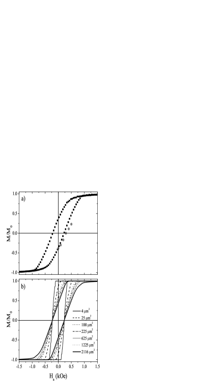
Figure 1: (a) Hysteresis loops as measured by SQUID with the external field applied parallel to the wire direction. The gray dots correspond to the magnetic moment deduced from the MFM images (see Sec. IV C). (b) Hysteresis loops performed by numerical simulations considering different sizes of the sample.

In order to understand the effect of the dipolar interactions on the hysteresis loop, we performed numerical simulations for the same array. From the measured value for $H_{c}$, we obtain $H_{ani}=2850\alpha$ Oe through Eq. (3) which defines $\alpha\approx 0.08$. By considering this value into the energy expression [Eq. (1)], we are in conditions to simulate the hysteresis loop. Monte Carlo simulations were carried out using Metropolis algorithm with local dynamics and single-spin-flip methods. Binder The initial state at $H_{a}$ $=2.0$ kOe, higher than the saturation field, considers the magnetization of all the wires aligned with the external field. The field was then linearly decreased at a rate of 300 Monte Carlo steps for $\Delta H=$ $0.01$ kOe. The new orientation of the magnetic nanowire was chosen arbitrarily with a probability $p=\min\left[1,exp(-\Delta E/k_{B}T)\right]$, where $\Delta E$ is the change in energy due to the reorientation of the wire, and $k_{B}$ is the Boltzmann constant. Figure 1(b) illustrates the hysteresis loop for samples with size ranging from $4$ $\mu$m² $\left(N=14\right)$ to $2116$ $\mu$m² $\left(N=9699\right)$. Each loop is the result of the average of five independent realizations. Because in our calculations the internal structure of the wire is not considered, the coercivity has a fix value independent of the number of wires in the array. From this figure, we can observe that the size of the sample strongly influences the shape of the loop as a whole and the particular role of the remanence. With present standard computational capabilities, it is not possible to obtain hysteresis loops with $N$ higher than $10000$. To describe the remanence of bigger arrays such as the ones experimentally investigated, we propose an alternative approach presented in next section.

IV.2 Remanent magnetization

In order to understand the role of the size of the sample, we calculate the dipolar interaction energy per wire for arrays of different sizes, $E_{int}=\sum_{i=1}^{N-1}\sum_{j=i+1}^{N}\left(D_{ij}/M_{0}N\right)$. By inspecting Fig. 1(b), we observed that it is possible to introduce a phenomenological analytical function that allows us to obtain the remanent magnetization as a function of the magnetostatic interaction present in the array. The reduced remanence $m_{r}$ can be written as

$$m_{r}=\frac{M_{r}}{M_{0}}=1-\frac{E_{int}}{\alpha}\text{ ,\ }$$ (4)

where $0\leq m_{r}\leq 1$. The dependence of calculated remanence $m_{r}$ (dotted line) and interaction energy $E_{int}$ (solid line) is depicted in Fig. 2 as a function of the size of the sample (i.e., number of nanowires $N$). Black dots illustrate $m_{r}$ obtained from the hysteresis loops shown in Fig. 1(b). For an array of $14400$ $\mu$m² $\left(N\approx 70000\right)$, the remanent magnetization converges to the value $m_{r}=0.38$, which is in excellent agreement with the remanence obtained with the SQUID measurements. These calculations establish a lower limit to the number of wires that have to be used in simulations to reach the experimental remanence value. Nevertheless, experimentally, it is not possible to measure arrays less than a few mm² in surface area with the required precision. At present, samples for experiments are $16$ mm², a size beyond saturation. Consequently, the theoretically established dependence of remanence on the sample size of such nanostructures is not yet experimentally confirmed. However, in the future, if smaller samples can be measured, it is important to consider this lower size limit.

Figure 2: Magnetostatic interaction per wire in the array (solid line) and remanent magnetization (dotted line) as a function of the size of the sample. Black dots correspond to the remanent magnetization obtained from hysteresis loops simulated in Fig. 1(b).

Now we further investigate the validity of Eq. 4 by calculating the remanence for different samples we found in the literature. Assuming that the size of the sample is big enough to reach convergence of the remanence, we use measured values of $H_{c}$ to calculate $\alpha$ and $m_{r}$ through Eqs. (3) and (4). In order to assure convergence, we fix $N=70000$. Table I summarizes the geometrical parameters of the array, $H_{c}$, $\alpha$ (which accounts for the influence of magnetic interactions in the reversal process and coercivity), the measured $m_{r}^{\ast}$, and calculated $m_{r}$ values of remanence. Note the agreement between experimental and calculated values through Eq. (4). Deviations between SQUID measurements and analytical results originated from the dispersion of the lengths and positions of each wire in the array and a reduction in the homogeneity of the diameter of nanopores. Vazquez2 Notice that in the sample defined by $d=55$ nm and $D=65$ nm, the wires are very close and then strong interactions are present between contiguous nanowires. Due to this interaction, the remanence decreases as evidenced in the measured and calculated values of the remanence in Table I.

Table 1: Parameters for different Ni nanowire arrays. Geometrical parameters, $H_{c}$, and $m_{r}^{\ast}$ have been measured in this paper [superscript 1] and taken from Ref. 28 [superscript 2] and Ref. 8 [superscript 3].

$d(nm)$	$D(nm)$	$L(\mu m)$	$H_{c}(Oe)$	$m_{r}^{\ast}$	$\alpha$	$m_{r}$
${}^{\left(1\right)}180$	$500$	$3.6$	$215$	$0.38$	$0.08$	$0.38$
${}^{\left(2\right)}25$	$65$	$2.5$	$720$	$0.70$	$0.24$	$0.80$
${}^{\left(2\right)}40$	$65$	$2.5$	$630$	$0.48$	$0.21$	$0.42$
${}^{\left(2\right)}55$	$65$	$2.5$	$420$	$0.10$	$0.14$	$0.00$
${}^{\left(2\right)}35$	$105$	$2.5$	$780$	$0.74$	$0.26$	$0.84$
${}^{\left(2\right)}50$	$105$	$2.5$	$680$	$0.70$	$0.23$	$0.66$
${}^{\left(3\right)}30$	$100$	$1.0$	$1200$	$0.99$	$0.41$	$0.92$
${}^{\left(3\right)}40$	$100$	$1.0$	$1000$	$0.80$	$0.35$	$0.83$
${}^{\left(3\right)}55$	$100$	$1.0$	$600$	$0.35$	$0.21$	$0.45$

IV.3 The patterned domain structure

MFM images have been obtained in different remanent states, since our MFM system permits us to apply magnetic fields in the course of the microscope operation.

The images in Fig. 3 illustrate different patterns obtained after applying increasing axial magnetic field. It is worth to mention that the MFM tip was previously saturated with positive field, in the same direction as the subsequent in situ applied magnetic field. The white contrast corresponds to nanowires with the magnetization oriented opposite to the tip field direction. When the magnetization of the nanowires points in the tip field direction, we obtain black contrast. The initial state [Fig. 3(a)] was achieved after magnetic saturation of the sample with a negative magnetic field. The images obtained after applying in situ magnetic fields of $90$, $190$, $290$, $400$, and $500$ Oe along the axial direction (see Figs. 3(b)-3(f), respectively) show us the evolution of the magnetic state of the individual nanowires. Notice the increment of the number of black nanowires after applying increasing magnetic field.

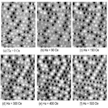
Figure 3: MFM images of the (a) initial state and after applying fields of (b) 90 Oe, (c) 190 Oe, (d) 290 Oe, (e) 400 Oe, and (f) 500 Oe parallel to the tip field.

In a previous report, Asenjo quantitative information of net magnetization from MFM images was analyzed. By counting the number of wires pointing in each direction, the remanent magnetization value, $m_{r}^{\ast}$can be obtained as

$$m_{r}^{\ast}=\frac{N_{w}-N_{b}}{N_{w}+N_{b}}\text{ ,}$$ (5)

where $N_{w}$ and $N_{b}$ are the numbers of wires with magnetization pointing up and down, respectively. Counting the black and white points in the MFM images in Fig. 3, $m_{r}^{\ast}$ was obtained for different values of $H_{a}$, which are illustrated with dots in Fig. 1(a). In the MFM results, the effect of the stray field of the tip must be taken into account. Moreover, since the images have been acquired in remanent states, the calculated magnetization values are slightly lower than the data obtained from the SQUID measurements.

Interactions play a fundamental role on the magnetically patterned structure of the samples. The patterned structure in an array, in principle, obeys to an antiferromagnetic-like alignment due to the magnetic interaction between the nanowires. As earlier reported Hwang for a square lattice, each of the four nearest neighbors aligns antiparallel and the magnetic structure of the array exhibits a checkerboard pattern. However, when we consider a typical hexagonal cell, as in Ref. 15, we have two almost degenerate states. At $T=$ 0, the configuration in Fig. 4(a) has, for d = 180 nm, D = 500 nm and L = 3.6 $\mu$m, a 10 % less energy than the configuration in Fig. 4(b). Due to such a small difference, the temperature, lattice disorder, or the magnetic history of the sample allows the array to exhibit any of both short-range configurations. Then, in a regular array, a mixture between both states is observed which originates the labyrinth pattern shown in Fig 4(c). This figure has been obtained by means of Monte Carlo simulations, as explained before, starting from a saturated sample and decreasing the external field until the coercive value. In this state, almost the same number of wires has their magnetization pointing up (white in Fig. 4) or down (black in Fig. 4), and nearest-neighbor parallel magnetic moments are organized in structures such as the ones shown in Fig. 4(a) and 4(b).

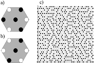
Figure 4: Magnetic configuration of a typical hexagonal cell with (a) minimum energy and (b) first excited state. Black (white) dots represent a wire with its magnetization pointing up (down). The energy difference between both configurations is 10 %. (c) Simulated patterned domain structure at remanence state. Image size: $15$ $\mu$m x $15$ $\mu$m.

A comparison between simulated and MFM labyrinth images confirms the at least qualitative agreement of this approach.

V Conclusions

In conclusion, by means of theoretical studies and experimental measurements, we have investigated the important role of magnetostatic interaction in the magnetic properties of nanowire arrays. We have derived an analytical expression that allows one to obtain the remanent magnetization as a function of the magnetostatic interactions presented in the array. Our results lead us to conclude that, because of the long-range order of the dipolar interactions between the wires, the size of the sample strongly influences the remanence of the array. In order to guarantee reproducibility, it is important to consider a sample which contains a minimum of 70000 wires. Also, the typical labyrinth pattern observed in the MFM images has been explained by a simple model considering the presence of two magnetic patterns of the basic cell of an hexagonal array. The MFM proves to be a useful method in studying the reversal magnetization process in nanostructures. Moreover, this powerful technique allows us to observe the individual evolution of the magnetic state of hundreds of nanowires under an external magnetic field. Good agreement between SQUID and MFM measurements and theoretical simulations is obtained.

VI Acknowledgments

This work has been partially supported by FONDECYT 1050013 and Millennium Science Nucleus Condensed Matter Physics P02-054F in Chile, and projects CAM GR/MAT/0437/2004 and PTR95/0935/OP in Spain. CONICYT Ph.D. Program, MECESUP USA0108 project, and Graduate Direction of Universidad de Santiago de Chile are also acknowledged. M.J. acknowledges the Comunidad Autonoma de Madrid for a FPI research grant. D.A. and J.E. are grateful to the Instituto de Ciencia de Materiales de Madrid-CSIC for the hospitality. We thank E. Salcedo for useful discussions.

References

- (1) C. A. Ross, Ann. Rev. Mater. Res. 31, 203 (2001).
- (2) J. I. Martin, J. Nogues, K. Liu, J. L. Vicent and I. K. Schuller, J. Magn. Magn. Mater. 256, 449 (2003).
- (3) G. Prinz, Science 282, 1660 (1998).
- (4) R. P. Cowburn and M. E. Welland, Science 287, 1466 (2000).
- (5) J. Escrig, P. Landeros, D. Altbir, E. E. Vogel and P. Vargas, J. Magn. Magn. Mater. 308, 233-237 (2007).
- (6) J. Escrig, P. Landeros, D. Altbir, M. Bahiana and J. d’Albuquerque e Castro, Appl. Phys. Lett. 89, 132501 (2006).
- (7) K. Nielsch, R. B. Wehrspohn, J. Barthel, J. Kirschner, S. F. Fischer, H. Kronmuller, T. Schweinbock, D. Weiss and U. Gosele, J. Magn. Magn. Mater. 291, 234-240 (2002).
- (8) K. Nielsch, R. B. Wehrspohn, J. Barthel, J. Kirschner, U. Gosele, S. F. Fischer and H. Kronmuller, Appl. Phys. Lett. 79, 1360 (2001).
- (9) M. Vázquez, K. Nielsch, P. Vargas, J. Velázquez, D. Navas, K. Pirota, M. Hernández-Vélez, E. Vogel, J. Catés, R. B. Wehrspohn and U. Gosele, Physica B 343, 395 (2004).
- (10) M. Vázquez, K. Pirota, J. Torrejón, D. Navas and M. Hernández-Vélez, J. Magn. Magn. Mater. 294, 174 (2005).
- (11) H. Masuda and K. Fukuda, Science 268, 1466 (1995).
- (12) R. Skomski, H. Zeng, M. Zheng and D. J. Sellmyer, Phys. Rev. B 62, 3900 (2000).
- (13) L. C. Sampaio, E. H. C. P. Sinnecker, G. R. C. Cernicchiaro, M. Knobel, M. Vázquez and J. Velázquez, Phys. Rev. B 61, 8976 (2000).
- (14) M. Knobel, L. C. Sampaio, E. H. C. P. Sinnecker, P. Vargas and D. Altbir, J. Magn. Magn. Mater. 249, 60 (2002).
- (15) R. Hertel, J. Appl. Phys. 90, 5752 (2001).
- (16) L. Clime, P. Ciureanu and A. Yelon, J. Magn. Magn. Mater. 297, 60 (2006).
- (17) M. Bahiana, F. S. Amaral, S. Allende and D. Altbir, Phys. Rev. B 74, 174412 (2006).
- (18) T. G. Sorop, C. Untiedt, F. Luis, M. Kroll, M. Rasa and L. J. de Jongh, Phys. Rev. B 67, 014402 (2003).
- (19) A. Asenjo, M. Jafaar, D. Navas and M. Vázquez, J. Appl. Phys. 100, 023909 (2006).
- (20) M. Vázquez, K. Pirota, M. Hernandez-Velez, V. M. Prida, D. Navas, R. Sanz, F. Batallan and J. Velazquez, J. Appl. Phys. 95, 6642 (2004).
- (21) A. Asenjo, D Garcia, J. M. Garcia, C. Prados and M. Vázquez, Phys. Rev. B 62, 6538 (2000).
- (22) M. Jaafar, A. Asenjo and M. Vázquez, Submitted to IEEE Trans. Nanotechnol. (2006).
- (23) M. Vázquez, M. Hernandez-Velez, K. Pirota, A. Asenjo, D. Navas, J. Velazquez, P. Vargas and C. Ramos, Eur. Phys. J. B 40, 489 (2004).
- (24) D. Laroze, J. Escrig, P. Landeros, D. Altbir, M. Vázquez and P. Vargas, Nanotechnology 18, 415708 (2007).
- (25) H. Kronmuller, K. D. Durst and M. Sagawa, J. Magn. Magn. Mater. 74, 291 (1988).
- (26) Marco Beleggia, Shakul Tandon, Yimei Zhu and Marc De Graef, J. Magn. Magn. Mater. 272-276, e1197-e1199 (2004).
- (27) K. Binder and D. Heermann, Monte Carlo Simulations in Statistical Physics (Springer, 2002).
- (28) D. Navas, Fabricación y caracterización de arreglos magnéticos en películas nanoporosas de alúmina anódica, Ph. D. Thesis Universidad Autónoma, (Julio 2006).
- (29) M. Hwang, M. C. Abraham, T. A. Savas, H. I. Smith, R. J. Ram and C. A. Ross, J. Appl. Phys. 87, 5108 (2000).