Supersymmetric Models for Neutrino Mass

Abstract

We review models for neutrino mass, with special emphasis in supersymmetric models where R–parity is broken either explicitly or spontaneously. The simplest unified extension of the MSSM with explicit bilinear R–parity violation provides a predictive scheme for neutrino masses and mixings which can account for the observed atmospheric and solar neutrino anomalies. Despite the smallness of neutrino masses R-parity violation is observable at present and future high-energy colliders, providing an unambiguous cross-check of the model. This model can be shown to be an effective model for the, more theoretically satisfying, spontaneous broken theory. The main difference in this last case is the appearance of a massless particle, the majoron, that can modify the decay modes of the Higgs boson, making it decay invisibly most of the time.

I Introduction

Despite the tremendous effort that has led to the discovery of neutrino mass [1, 2, 3] the mechanism of neutrino mass generation will remain open for years to come (a detailed analysis of the three–neutrino oscillation parameters can be found in  [4]). The most popular mechanism to generate neutrino masses is the seesaw mechanism [5, 6, 7, 8, 9, 10, 11, 12]. Although the seesaw fits naturally in SO(10) unification models, we currently have no clear hints that uniquely point towards any unification scheme.

Therefore it may well be that neutrino masses arise from physics having nothing to do with unification, such as certain seesaw variants [13], and models with radiative generation [14, 15]. Here we focus on the specific case of low-energy supersymmetry with violation of R–parity, as the origin of neutrino mass. R–parity is defined as $R_{p}=(-1)^{3B+L+2S}$ with $S$, $B$, $L$ denoting spin, baryon and lepton numbers, respectively [16].

In these models R–parity can be broken either explicitly or spontaneously. In the first case we consider the bilinear R–parity violation (BRpV) model, the simplest effective description of R-parity violation [17]. The model not only accounts for the observed pattern of neutrino masses and mixing [18, 19, 20, 21], but also makes predictions for the decay branching ratios of the lightest supersymmetric particle [22, 23, 24, 25] from the current measurements of neutrino mixing angles [4]. In the second case R–parity violation takes place “a la Higgs”, i.e., spontaneously, due to non-zero sneutrino vacuum expectation values (vevs) [26, 27, 28]. In this case one of the neutral CP-odd scalars is identified with the majoron, $J$. In contrast with the seesaw majoron, ours is characterized by a small scale (TeV-like) and carries only one unit of lepton number. In previous studies [29, 30, 31, 32] it was noted that the spontaneously R–parity violation (SRpV) model leads to the possibility of invisibly decaying Higgs bosons, provided there is an SU(2) $\otimes$ U(1) singlet superfield $\Phi$ coupling to the electroweak doublet Higgses, the same that appears in the NMSSM. We have reanalyzed [33, 34] this issue taking into account the small masses indicated by current neutrino oscillation data [4]. We have shown explicitly that the invisible Higgs boson decay Eq. (1),

$$h\to JJ$$ (1)

can be the most important mode of Higgs boson decay. This is remarkable, given the smallness of neutrino masses required to fit current neutrino oscillation data.

II Models for Neutrino Mass

In 1980, Weinberg[35] noticed that the dimension-five operator

$$\mathcal{L}_{\rm Dim5}=L\phi\,L\phi$$ (2)

could induce neutrino masses:

\psfrag{n}{$\nu_{L}$}\psfrag{f}{$\left\langle\phi\right\rangle$}\includegraphics[height=71.13188pt]{dimensionfive.eps}

The models that can lead to this type of operator can be classified in Seesaw Models and Radiative Models, that we now briefly review.

II-A Seesaw models for neutrino mass

II-A1 Type I mechanism

In models with right handed neutrinos

$$-\mathcal{L}=\overline{\nu_{L}}m_{D}\nu_{R}+\frac{1}{2}\overline{\nu_{L}^{c}}M_{R}\nu_{R}$$ (3)

where $m_{D}=Y_{\nu}v$. The seesaw (Type I) [5, 6, 7, 10, 11] formula is

$$m_{\rm eff}^{\rm I}=-(vY_{\nu})M_{R}^{-1}(vY_{\nu})^{T}$$ (4)

which corresponds to the following diagram:

\psfrag{nL}{$\nu_{L}$}\psfrag{nR}{$\nu_{R}$}\psfrag{MR}{$M_{R}$}\psfrag{f}{$\left\langle\phi\right\rangle$}\includegraphics[clip,height=71.13188pt]{typeI.eps}

II-A2 Type II mechanism

In models with Higgs triplets

$$-\mathcal{L}=\frac{1}{2}Y_{\Delta}\overline{\nu_{L}^{c}}i\tau_{2}\Delta_{L}\nu_{L}+\mu\phi^{T}\Delta_{L}\phi+M^{2}_{\Delta}\Delta_{L}^{\dagger}\Delta_{L}+\cdots$$ (5)

we obtain the type II seesaw formula [8, 10, 11, 36]

$$m_{\rm eff}^{\rm II}=\frac{v^{2}\mu Y_{\Delta}}{M^{2}_{\Delta}}$$ (6)

which corresponds to the following diagram

\psfrag{nL}{$\nu_{L}$}\psfrag{nR}{$\nu_{R}$}\psfrag{MR}{$M_{R}$}\psfrag{f}{$\left\langle\phi\right\rangle$}\psfrag{D}{$\Delta^{0}$}\psfrag{m}{$\mu$}\psfrag{YD}{$Y_{\Delta}$}\includegraphics[height=71.13188pt]{typeII.eps}

II-A3 Inverse Seesaw

In addition to the normal neutrinos $\nu_{L}$, the inverse seesaw[13] uses two sequential SU(3) $\otimes$ SU(2) $\otimes$ U(1) singlets $\nu_{L}^{c}$, $S_{L}$, corresponding to the following mass matrix

$$M_{\nu}=\left(\begin{array}[]{ccc}0&Y_{\nu}v&0\\ Y_{\nu}^{T}v&0&M\\ 0&M&\mu\end{array}\right)$$ (7)

where $Y_{\nu}$ are Yukawa couplings, $M$ and $\mu$ are SU(3) $\otimes$ SU(2) $\otimes$ U(1) invariant mass entries. The effective mass matrix is then

$$m_{\rm eff}^{\rm Inv}=-v^{2}(Y{M^{T}}^{-1})\mu({M}^{-1}Y^{T})$$ (8)

The smallness of $\mu$ is natural, in t’Hooft’s sense. However, there is no dynamical understanding of this smallness.

II-A4 A Supersymmetric SO(10) Inverse Seesaw

We proposed[12] an alternative inverse seesaw consistent with a realistic unified SO(10) model. In this model the mass matrix reads

$$M_{\nu}=\left(\begin{array}[]{ccc}0&Yv&Fv_{L}\\ Y^{T}v&0&\tilde{F}v_{R}\\ F^{T}v_{L}&\tilde{F}^{T}v_{R}&0\end{array}\right)$$ (9)

By inserting $v_{L}=\rho\frac{v_{R}v}{M_{G}}$, coming from the minimization conditions[12], the $v_{R}$ scale drops out, leading to

$$m_{\rm eff}^{\rm NewInv}\simeq\frac{v^{2}}{M_{G}}\rho\left[Y(F\tilde{F}^{-1})^{T}+(F\tilde{F}^{-1})Y^{T}\right]$$ (10)

The neutrino mass is suppressed by $M_{G}$, irrespective of how low is the B-L breaking scale $v_{R}$ (as low as few TeV). This corresponds to the following diagram

This new seesaw is linear in the Dirac Yukawa couplings $Y$. The most important result is that a low $B-L$ scale can be achieved while preserving the gauge coupling unification as shown in Fig. 1.

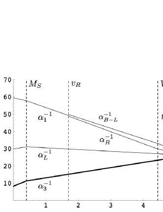
Figure 1: Gauge coupling unification in the in model of Ref.[12].

Another important result is the calculation of the CP asymmetry needed for leptogenesis in a model that is a variant[37] of the previous one. The results[38] are shown in Fig. 2.

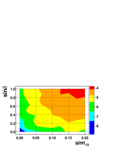
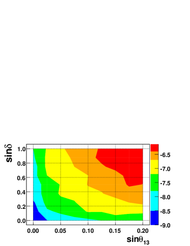
Figure 2: Contour levels of the maximum value of the asymmetry $\epsilon_{\Sigma}$ obtained as a function of $\sin\theta_{13}$ and $\sin\delta$. For details see Ref.[38].

II-B Models with radiatively generated neutrino mass

II-B1 Zee Model

In the Zee model[14], the scalar sector of the model consists of two Higgs doublets with the same hypercharge and a charged $SU(2)$ scalar singlet $h^{\pm}$, with $L(h^{-})=2$.

$${\cal L}_{Y}=\bar{L}_{i}(\Pi_{a})_{ij}\Phi_{a}e_{Rj}+\epsilon_{\alpha\beta}\bar{L}^{\alpha}_{i}f_{ij}\,C(\bar{L}^{T})^{\beta}_{j}h^{-}+\hbox{h.c.}$$ (11)

Therefore Yukawa interactions conserve $L$, which is explicitly broken in the scalar potential

$$V\supset\mu\epsilon_{\alpha\beta}\Phi_{1}^{\alpha}\Phi_{2}^{\beta}h^{-}+\mbox{h.c.}$$ (12)

Charged scalar mixing and Yukawa interactions generate neutrino masses at the one loop level through the diagram

\psfrag{n}{$\nu$}\psfrag{hp}{$h^{+}$}\psfrag{hm}{$h^{-}$}\psfrag{l}{$l$}\psfrag{lb}{$\overline{l}$}\includegraphics{zee.eps}

II-B2 Babu-Zee Model

Apart from the Higgs doublet the model[15, 39], contains a single charged and a doubly charged ($h^{+}$, $k^{++}$) $SU(2)$ gauge singlets scalars. In contrast to the Zee model the second Higgs doublet is absent. We have

$${\cal L}=f_{\alpha\beta}(L^{Ti}_{\alpha L}CL^{j}_{\beta L})\epsilon_{ij}h^{+}+h^{\prime}_{\alpha\beta}(e^{T}_{\alpha R}Ce_{\beta R})k^{++}+{\rm h.c.}$$ (13)

with $L(h^{-})=L(k^{--})=2$. Therefore the Lagrangian conserves $L$, which is explicitly broken in the scalar potential

$$V\supset\mu k^{++}h^{-}h^{-}$$ (14)

Yukawa interactions and the breaking of Lepton number, generate Majorana neutrino masses at the 2-loop level, as indicated in the following diagram:

II-B3 Broken R-Parity Models

R–parity is defined in supersymmetric theories by the relation

$$R_{P}=(-1)^{2J+3B+L}$$ (15)

Although the MSSM is defined to conserve R–parity, there is no fundamental principle that requires that. If it is not conserved it can broken in two ways

• BRpV: Explicit R-parity Violation

  In this case R–parity is broken at the Lagrangian level. The most important example is the so-called Bilinear R–parity Violation (BRpV) model which has the same particle content as the MSSM.

• SRpV: Spontaneously R-parity Violation

  In this case we have a more complicated Higgs boson structure. The most salient feature is the existence of the Majoron $J$, the massless Goldstone boson appearing due to the spontaneous breaking of R–parity.

In the next sections we will review in more detail these two ways of generating neutrino masses and we will indicate ways of testing these ideas at accelerators.

III Bilinear R-Parity Violation

III-A The model

This model[40, 41] has the same particle content as the MSSM. The superpotential $W$ is

$$W = \varepsilon_{ab}\left[h_{U}^{ij}\widehat{Q}_{i}^{a}\widehat{U}_{j}\widehat{H}_{u}^{b}+h_{D}^{ij}\widehat{Q}_{i}^{b}\widehat{D}_{j}\widehat{H}_{d}^{a}+h_{E}^{ij}\widehat{L}_{i}^{b}\widehat{R}_{j}\widehat{H}_{d}^{a}\right.$$ (17)

$$\left.\hskip 28.45274pt-\mu\widehat{H}_{d}^{a}\widehat{H}_{u}^{b}+\epsilon_{i}\widehat{L}_{i}^{a}\widehat{H}_{u}^{b}\right]$$

where $i,j=1,2,3$ are generation indices, $a,b=1,2$ are $SU(2)$ indices. The set of soft supersymmetry breaking terms are

$$V_{soft}=V_{soft}^{\textrm{MSSM}}+\varepsilon_{ab}\ B_{i}\epsilon_{i}\widetilde{L}^{a}_{i}H_{u}^{b}$$ (18)

III-B Tree Level: Atmospheric Mass Scale

In the basis: $\psi^{0T}=(-i\lambda^{\prime},-i\lambda^{3},\widetilde{H}_{d}^{1},\widetilde{H}_{u}^{2},\nu_{e},\nu_{\mu},\nu_{\tau})$ the mass matrix reads[19, 20]

$${\kern-0.24994pt\hbox{$M$}\kern-10.79166pt\kern 0.50003pt\hbox{$M$}\kern-10.79166pt\kern-0.24994pt\raise 0.43304pt\hbox{$M$}}_{N}\hskip-2.84526pt=\hskip-2.84526pt\left[\hskip-4.2679pt\begin{array}[]{cc}{\cal M}_{\chi^{0}}&m^{T}\cr\vbox to20.0pt{}m&0\cr\end{array}\hskip-2.84526pt\right]\hskip-2.84526pt;m=\hskip-2.84526pt\left[\hskip-2.84526pt\begin{array}[]{cccc}-\frac{1}{2}g^{\prime}v_{1}&\frac{1}{2}gv_{1}&0&\epsilon_{1}\cr-\frac{1}{2}g^{\prime}v_{2}&\frac{1}{2}gv_{2}&0&\epsilon_{2}\cr-\frac{1}{2}g^{\prime}v_{3}&\frac{1}{2}gv_{3}&0&\epsilon_{3}\cr\end{array}\hskip-2.84526pt\right]$$ (19)

which gives the effective mass matrix

$$m_{eff} \hskip-5.69054pt= \hskip-5.69054pt-m\,{\cal M}_{\chi^{0}}^{-1}\,m^{T}$$ (23)

$$\hskip-5.69054pt=\hskip-5.69054pt \frac{M_{1}g^{2}+M_{2}{g^{\prime}}^{2}}{4\textrm{det}({\cal M}_{\chi^{0}})}\left(\hskip-5.69054pt\begin{array}[]{ccc}\Lambda_{e}^{2}&\Lambda_{e}\Lambda_{\mu}&\Lambda_{e}\Lambda_{\tau}\\ \Lambda_{e}\Lambda_{\mu}&\Lambda_{\mu}^{2}&\Lambda_{\mu}\Lambda_{\tau}\\ \Lambda_{e}\Lambda_{\tau}&\Lambda_{\mu}\Lambda_{\tau}&\Lambda_{\tau}^{2}\end{array}\hskip-5.69054pt\right)$$

where $\Lambda_{i}=\mu v_{i}+v_{d}\epsilon_{i}$. This effective mass matrix has two massless neutrinos and one massive neutrino with mass[19]

$$m_{\nu}=Tr(m_{eff})=\displaystyle\frac{M_{1}g^{2}+M_{2}{g^{\prime}}^{2}}{4\,\textrm{det}({\cal M}_{\chi^{0}})}|{\vec{\Lambda}}|^{2}.$$ (24)

III-C One Loop: Solar Mass Scale

In this model the solar neutrino mass is generated at one loop level. The most important contributions come[18] from the bottom-sbottom loops indicated in Fig. 3.

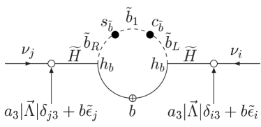
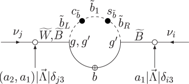
Figure 3: Bottom-sbottom loops generating the neutrino masses. In this Figure open circles correspond to small R-parity violating projections, full circles correspond to R-parity conserving projections and open circles with a cross inside to mass insertions which flip chirality.

In Fig. 4 we show an example of neutrino masses as function of the BRpV parameters.

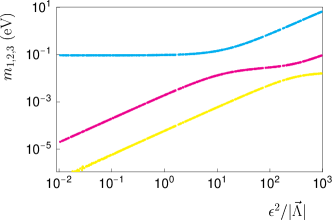
Figure 4: Neutrino masses in the BRpV for the following values of the MSSM parameters:$m_{0}=\mu=500$ GeV, $\tan\beta=5$, $B=-A=m_{0}$. The range of BRpV parameters is as follows: $|\vec{\Lambda}|=0.16$ GeV, $10*\Lambda_{e}=\Lambda_{\mu}=\Lambda_{\tau}$ and $\epsilon_{1}=\epsilon_{2}=\epsilon_{3}$

IV Spontaneous Broken R-Parity

IV-A The model

The most general superpotential that leads to Spontaneous R-parity Violation (SRpV) is

$${\cal W} \hskip-11.38109pt=\hskip-11.38109pt \varepsilon_{ab}\Big{(}h_{U}^{ij}\widehat{Q}_{i}^{a}\widehat{U}_{j}\widehat{H}_{u}^{b}+h_{D}^{ij}\widehat{Q}_{i}^{b}\widehat{D}_{j}\widehat{H}_{d}^{a}+h_{E}^{ij}\widehat{L}_{i}^{b}\widehat{E}_{j}\widehat{H}_{d}^{a}$$ (25)

$$+h_{\nu}^{ij}\widehat{L}_{i}^{a}\widehat{\nu}^{c}_{j}\widehat{H}_{u}^{b}\!-{\hat{\mu}}\widehat{H}_{d}^{a}\widehat{H}_{u}^{b}\!-(h_{0}\widehat{H}_{d}^{a}\widehat{H}_{u}^{b}+\delta^{2})\widehat{\Phi}\Big{)}$$

$$+h^{ij}\widehat{\Phi}\widehat{\nu}^{c}_{i}\widehat{S}_{j}+M_{R}^{ij}\widehat{\nu}^{c}_{i}\widehat{S}_{j}+\frac{1}{2}M_{\Phi}\widehat{\Phi}^{2}+\frac{\lambda}{3!}\widehat{\Phi}^{3}$$

where the singlet superfields $({\nu^{c}}_{i},S_{i},\Phi)$ carry a conserved lepton number assigned as $(-1,1,0)$. Therefore Lepton number and R-parity are conserved at Lagrangian Level.

IV-B SRpV: Symmetry Breaking

The spontaneous breaking of R–parity is driven by nonzero vevs for the scalar neutrinos. The scale characterizing R–parity breaking is set by the isosinglet vevs

$$\left\langle\tilde{\nu^{c}}\right\rangle=\frac{v_{R}}{\sqrt{2}},\quad\left\langle\tilde{S}\right\rangle=\frac{v_{S}}{\sqrt{2}},\quad\left\langle\Phi\right\rangle=\frac{v_{\Phi}}{\sqrt{2}}$$ (26)

We also have very small left-handed sneutrino vacuum expectation values

$$\left\langle\tilde{\nu}_{Li}\right\rangle=\frac{v_{Li}}{\sqrt{2}}$$ (27)

The electroweak breaking is driven by

$$\left\langle{H_{u}}\right\rangle=\frac{v_{u}}{\sqrt{2}},\quad\left\langle{H_{d}}\right\rangle=\frac{v_{d}}{\sqrt{2}}$$ (28)

with $v^{2}=v_{u}^{2}+v_{d}^{2}+\sum_{i}v_{Li}^{2}$ and $m_{W}^{2}=\frac{g^{2}v^{2}}{4}$. The spontaneous breaking of R–parity also entails the spontaneous violation of total lepton number. This implies that the Majoron

$$J=\mathrm{Im}\left[\displaystyle\frac{v_{L}^{2}}{Vv^{2}}(v_{u}H_{u}-v_{d}H_{d})+\sum_{i}\frac{v_{Li}}{V}\tilde{\nu_{i}}+\frac{v_{S}}{V}S-\frac{v_{R}}{V}\tilde{\nu^{c}}\right]$$ (29)

remains massless, as it is the Nambu-Goldstone boson associated to the breaking of lepton number.

IV-C SRpV: The effective neutrino mass matrix

The effective neutrino mass matrix can be cast into a very simple form

$$(\mathbf{m_{\nu\nu}^{\rm eff}})_{ij}=a\Lambda_{i}\Lambda_{j}+b(\epsilon_{i}\Lambda_{j}+\epsilon_{j}\Lambda_{i})+c\epsilon_{i}\epsilon_{j}.$$ (30)

This equation resembles very closely the result for the BRpV model once the dominant 1-loop corrections are taken into account. The effective bilinear R–parity violating parameters are

$$\epsilon_{i}=h_{\nu}^{i}\,\frac{v_{R}}{\sqrt{2}}\quad\hbox{and}\quad\Lambda_{i}=\epsilon_{i}v_{d}+\mu v_{L_{i}}$$ (31)

V Tests of the Bilinear R-Parity Violation Model

V-A Testing BRpV via SUSY Decays

• LSP Decays: (mSUGRA)

  The fact that, in these models, the LSP decays through R–parity violating processes allows it to be either neutral or charged.

  • In most cases the LSP is the lightest neutralino, like in the MSSM[23].

  • For some regions of the parameter space the LSP can also be the scalar tau[22].

  • In both cases we have shown that despite the smallness of $m_{\nu}$ the LSP decays inside the detector.

• LSP Decays: (non mSUGRA)

  If we depart from mSUGRA then the LSP can be almost any particle[25]. This gives complementary information.

V-B Neutralino decays: Probing the Atmospheric Angle

When the LSP is the neutralino the ratios of branching ratios can be correlated with the neutrino parameters. For instance, in Fig. 5 we show[23] the correlation with the atmospheric angle.

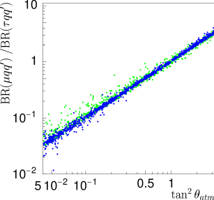
Figure 5: Relation of branching of branching ratios of neutralino decays and the atmospheric angle (Ref. [23]).

The spread in Fig. 5 will disappear if the SUSY parameters were known, as it is indicated in Fig. 6.

Figure 6: Same as in Fig. 5, but assuming that SUSY has been discovered with $M_{2}=120\,\hbox{GeV},\mu=500\,\hbox{GeV},\tan\beta=5$ $m_{0}=500\,\hbox{GeV},A=-500\,\hbox{GeV}$ (Ref. [23]).

V-C Stau Decays and the Solar Angle

In the region of parameters space where the LSP is the stau we can use its decays[22], to make correlations to the neutrino parameters as is indicated in Fig. 7.

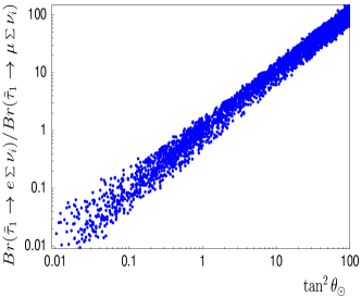
Figure 7: Correlations of the stau decays with the solar angle (Ref. [22]).

V-D Other LSP Decays (depart from mSUGRA)

If we depart from mSUGRA then the LSP can be almost any particle. For instance, it was shown in Ref.[25] that you can correlate the decays of charginos and squarks with the neutrino parameters. In Fig. 8 and Fig. 9 we show, respectively the case of the LSP being the chargino or the squark.

Figure 8: Correlations for the atmospheric parameters when the LSP is the chargino (Ref. [25]).

Figure 9: Correlations for the solar angle when the LSP is the squark (Ref. [25]).

VI Tests of the Spontaneous R-Parity Violation Model

VI-A Higgs Boson Production

Supersymmetric Higgs bosons can be produced at the $e^{+}e^{-}$ collider via the so–called Bjorken process, coming from the coupling

$${\cal L}_{HZZ}=\displaystyle\sum_{i=1}^{8}(\sqrt{2}G_{F})^{1/2}M_{Z}^{2}Z_{\mu}Z^{\mu}\eta_{i}H_{i}$$ (32)

where the $\eta_{i}$ are a combination of the doublet scalars,

$$\eta_{i}=\frac{v_{d}}{v}\ R^{S}_{i1}+\frac{v_{u}}{v}\ R^{S}_{i2}+\sum_{j=1}^{3}\frac{v_{Lj}}{v}\ R^{S}_{ij+2}$$ (33)

and the $R^{S}_{ij}$ are rotation matrices that diagonalize the CP even neutral Higgs bosons. In comparison with the SM, the coupling of the lightest CP–even Higgs boson to the $Z$ is reduced by

$$\eta\equiv\eta_{1}\leq 1$$ (34)

VI-B Higgs Boson Decay

We are interested here in the ratio

$$R_{Jb}=\displaystyle\frac{\Gamma(h\to JJ)}{\Gamma(h\to b\bar{b})}$$ (35)

of the invisible decay to the SM decay into b-jets. These decay widths are

$$\Gamma(h\to JJ)=\displaystyle\frac{g_{hJJ}^{2}}{32\pi m_{h}}$$ (36)

and

$$\hskip-2.84526pt\Gamma(h\to b\bar{b})=\frac{3G_{F}\sqrt{2}}{8\pi}\!\!\left(R^{S}_{11}\right)^{2}\!m_{h}m_{b}^{2}\left[\!1\!-\!4\left(\frac{m_{b}}{m_{h}}\right)^{2}\!\right]^{3/2}$$ (37)

VI-C Numerical results

We have performed a careful analysis of the SBpV model in order to search for the possibility of having at the same time a large branching ratio of the Higgs boson into the invisible channel of the Majoron and at the same time the production cross section to be not too much reduced with respect to the SM case. The conclusion[33, 34] is that this is indeed possible as is shown, as an example in Fig. 10. All the points in these curves respect the neutrino data[4].

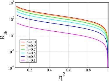
Figure 10: $R_{Jb}$ vs $\eta^{2}$ for fixed $h$ from Ref.[33]. See text, Eq. (33), Eq. (35) and Eq. (25) for an explanation of these quantities.

VII Conclusions

We have briefly reviewed the models for neutrino mass. In the class of seesaw models we discussed in some detail the implications of a new seesaw model that can achieve successful leptogenesis and can have low energy implications. Among the radiative models we have focused on those with broken R-parity. We have considered both the models with explicit R-parity violation (BRpV) and also models with spontaneous violation of R-parity (SRpV). Both possibilities have implications at the new accelerators and therefore can be tested in the upcoming machines.

References

- [1] Super-Kamiokande, Y. Fukuda et al., Phys. Rev. Lett. 81, 1562 (1998), [hep-ex/9807003].
- [2] SNO, Q. R. Ahmad et al., Phys. Rev. Lett. 89, 011301 (2002), [nucl-ex/0204008].
- [3] KamLAND, K. Eguchi et al., Phys. Rev. Lett. 90, 021802 (2003), [hep-ex/0212021].
- [4] M. Maltoni, T. Schwetz, M. A. Tortola and J. W. F. Valle, New J. Phys. 6, 122 (2004), [hep-ph/0405172].
- [5] P. Minkowski, Phys. Lett. B67, 421 (1977).
- [6] M. Gell-Mann, P. Ramond and R. Slansky, (1979), Print-80-0576 (CERN).
- [7] T. Yanagida, (1979), ed. Sawada and Sugamoto (KEK, 1979).
- [8] R. N. Mohapatra and G. Senjanovic, Phys. Rev. D23, 165 (1981).
- [9] Y. Chikashige, R. N. Mohapatra and R. D. Peccei, Phys. Lett. B98, 265 (1981).
- [10] J. Schechter and J. W. F. Valle, Phys. Rev. D22, 2227 (1980).
- [11] G. Lazarides, Q. Shafi and C. Wetterich, Nucl. Phys. B181, 287 (1981).
- [12] M. Malinsky, J. C. Romao and J. W. F. Valle, Phys. Rev. Lett. 95, 161801 (2005), [hep-ph/0506296].
- [13] R. N. Mohapatra and J. W. F. Valle, Phys. Rev. D34, 1642 (1986).
- [14] A. Zee, Phys. Lett. B93, 389 (1980).
- [15] K. S. Babu, Phys. Lett. B203, 132 (1988).
- [16] C. S. Aulakh and R. N. Mohapatra, Phys. Lett. B119, 136 (1982).
- [17] M. A. Diaz, J. C. Romao and J. W. F. Valle, Nucl. Phys. B524, 23 (1998), [hep-ph/9706315].
- [18] M. A. Diaz, M. Hirsch, W. Porod, J. C. Romao and J. W. F. Valle, Phys. Rev. D68, 013009 (2003), [hep-ph/0302021].
- [19] J. C. Romao, M. A. Diaz, M. Hirsch, W. Porod and J. W. F. Valle, Phys. Rev. D61, 071703 (2000), [hep-ph/9907499].
- [20] M. Hirsch, M. A. Diaz, W. Porod, J. C. Romao and J. W. F. Valle, Phys. Rev. D62, 113008 (2000), [hep-ph/0004115].
- [21] M. Hirsch and J. W. F. Valle, New J. Phys. 6, 76 (2004), [hep-ph/0405015].
- [22] M. Hirsch, W. Porod, J. C. Romao and J. W. F. Valle, Phys. Rev. D66, 095006 (2002), [hep-ph/0207334].
- [23] W. Porod, M. Hirsch, J. Romao and J. W. F. Valle, Phys. Rev. D63, 115004 (2001), [hep-ph/0011248].
- [24] D. Restrepo, W. Porod and J. W. F. Valle, Phys. Rev. D64, 055011 (2001), [hep-ph/0104040].
- [25] M. Hirsch and W. Porod, Phys. Rev. D68, 115007 (2003), [hep-ph/0307364].
- [26] A. Masiero and J. W. F. Valle, Phys. Lett. B251, 273 (1990).
- [27] J. C. Romao, C. A. Santos and J. W. F. Valle, Phys. Lett. B288, 311 (1992).
- [28] M. Shiraishi, I. Umemura and K. Yamamoto, Phys. Lett. B313, 89 (1993).
- [29] J. C. Romao and J. W. F. Valle, Nucl. Phys. B381, 87 (1992).
- [30] J. C. Romao, F. de Campos and J. W. F. Valle, Phys. Lett. B292, 329 (1992), [hep-ph/9207269].
- [31] F. De Campos, J. W. F. Valle, A. Lopez-Fernandez and J. C. Romao, hep-ph/9405382.
- [32] F. de Campos, O. J. P. Eboli, J. Rosiek and J. W. F. Valle, Phys. Rev. D55, 1316 (1997), [hep-ph/9601269].
- [33] M. Hirsch, J. C. Romao, J. W. F. Valle and A. Villanova del Moral, Phys. Rev. D70, 073012 (2004), [hep-ph/0407269].
- [34] M. Hirsch, J. C. Romao, J. W. F. Valle and A. Villanova del Moral, Phys. Rev. D73, 055007 (2006), [hep-ph/0512257].
- [35] S. Weinberg, Phys. Rev. D22, 1694 (1980).
- [36] J. Schechter and J. W. F. Valle, Phys. Rev. D25, 774 (1982).
- [37] M. Hirsch, J. W. F. Valle, M. Malinsky, J. C. Romao and U. Sarkar, Phys. Rev. D75, 011701 (2007), [hep-ph/0608006].
- [38] J. C. Romao, M. A. Tortola, M. Hirsch and J. W. F. Valle, arXiv:0707.2942 [hep-ph].
- [39] A. Zee, Nucl. Phys. B264, 99 (1986).
- [40] A. G. Akeroyd, M. A. Diaz, J. Ferrandis, M. A. Garcia-Jareno and J. W. F. Valle, Nucl. Phys. B529, 3 (1998), [hep-ph/9707395].
- [41] M. A. Diaz, J. C. Romao and J. W. F. Valle, Nucl. Phys. B524, 23 (1998), [hep-ph/9706315].