Abstract

We consider a complex version of the $\vee$-systems, which appeared in the theory of the WDVV equation. We show that the class of these systems is closed under the natural operations of restriction and taking the subsystems and study a special class of the $\vee$-systems related to generalized root systems and basic classical Lie superalgebras.

1 Introduction

The main object of our study is the special collections of vectors in a linear space, which are called $\vee$-systems. They were introduced in [1, 2] in relation with a certain class of special solutions of the generalized Witten-Dijkgraaf-Verlinde-Verlinde (WDVV) equations, playing an important role in 2D topological field theory and $N=2$ SUSY Yang-Mills theory [3, 4]. A geometric theory of the WDVV equation was developed by Dubrovin, who introduced a fundamental notion of Frobenius manifold [3, 5].

The definition of the $\vee$-systems is as follows. Let for beginning $V$ be a real vector space and $\mathcal{A}\subset V^{*}$ be a finite set of vectors in the dual space $V^{*}$ (covectors) spanning $V^{*}$. To such a set one can associate the following canonical form $G_{\mathcal{A}}$ on $V$:

$$G_{\mathcal{A}}(x,y)=\sum_{\alpha\in\mathcal{A}}\alpha(x)\alpha(y),$$

where $x,y\in V$. This is a non-degenerate scalar product, which establishes the isomorphism

$$\varphi_{\mathcal{A}}:V\rightarrow V^{*}.$$

The inverse $\varphi_{\mathcal{A}}^{-1}(\alpha)$ we denote as $\alpha^{\vee}$. The system $\mathcal{A}$ is called $\vee$-system if the following relations (called $\vee$-conditions)

$$\sum\limits_{\beta\in\Pi\cap\mathcal{A}}\beta(\alpha^{\vee})\beta^{\vee}=\lambda\alpha^{\vee}$$

are satisfied for any $\alpha\in\mathcal{A}$ and any two-dimensional plane $\Pi\subset V^{*}$ containing $\alpha$ and some $\lambda$, which may depend on $\Pi$ and $\alpha.$ For more geometric definition and the relation to WDVV equation see [1, 2] and the next section.

One can show [1] that all Coxeter root systems as well as their deformed versions appeared in the theory of quantum Calogero-Moser systems satisfy these conditions (see also [6, 7], where the relation between $\vee$-systems and Calogero-Moser theory was clarified).

In this paper we study the geometric properties of $\vee$-systems in more detail. In particular we show that a subsystem of the $\vee$-system is also a $\vee$-system, the result which we announced in [8]. This may be not surprising but not obvious from the definition.

A surprising fact is that the restriction of a $\vee$-system $\mathcal{A}$ to the subspace defined by a subset $\mathcal{B}\subset\mathcal{A}$ is also a $\vee$-system (see [9]). This is clearly not true for the Coxeter root systems. In fact, $\vee$-systems can be considered as an extension of the class of Coxeter systems, which has this property.

We show that all these properties (under some mild additional assumptions) are true also for a natural complex version of the $\vee$-systems, which we discuss in the next section. The consideration of the complex $\vee$-systems was partly motivated by the link with the theory of Lie superalgebras developed in [10]. We study the new examples of the $\vee$-systems coming from this theory in relation with the restrictions of Coxeter root systems investigated in [9].

In the last section we discuss complex Euclidean $\vee$-systems, which is an extension of the class of $\vee$-systems, when the canonical form is allowed to be degenerate. The root systems of some basic classical Lie superalgebras give important examples of such systems.

We finish with the list of all known $\vee$-systems in dimension 3.

2 Complex $\vee$-systems and WDVV equation

Let now $V$ be a complex vector space and $\mathcal{A}\subset V^{*}$ be a finite set of covectors. We will assume that the bilinear form on $V$

$$G_{\mathcal{A}}(x,y)=\sum_{\alpha\in\mathcal{A}}\alpha(x)\alpha(y)$$ (1)

is non-degenerate. In the real case this would simply mean that the elements of $\mathcal{A}$ span $V^{*}$, in the complex case our assumption is stronger. This form then establishes the isomorphism

$$\varphi_{\mathcal{A}}:V\rightarrow V^{*}.$$

We denote $\alpha^{\vee}=\varphi_{\mathcal{A}}^{-1}(\alpha)$ and say in full analogy with the real case [1] that $\mathcal{A}$ is a $\vee$-system if for any $\alpha\in\mathcal{A}$ and for any two-dimensional plane $\pi$ containing $\alpha$ the following $\vee$-condition holds

$$\sum_{\beta\in\pi\cap\mathcal{A}}\beta(\alpha^{\vee})\beta^{\vee}=\lambda\alpha^{\vee}$$ (2)

for some constant $\lambda=\lambda(\alpha,\pi)$. Equivalently one can say that either subsystem $\Pi=\pi\cap\mathcal{A}$ is reducible in the sense that it consists of two orthogonal subsystems or the following forms are proportional:

$$G_{\Pi}|_{\pi^{\vee}\times V}\sim G_{\mathcal{A}}|_{\pi^{\vee}\times V},$$

where

$$G_{\Pi}(x,y)=\sum_{\beta\in\Pi\cap\mathcal{A}}\beta(x)\beta(y).$$ (3)

Originally $\vee$-systems in $\mathbb{R}^{n}$ appeared as geometric reformulation of the Witten-Dijkgraaf-Verlinde-Verlinde equations for the prepotential

$$F=\sum_{\alpha\in\mathcal{A}}\alpha(x)^{2}\log\alpha(x)^{2},$$ (4)

but the proof [1] was using some geometry of the real plane. We will show now that one can avoid this and that similar interpretation holds in the complex case as well.

Recall first that the (generalized) WDVV equations have the form

$$F_{i}F_{j}^{-1}F_{k}=F_{k}F_{j}^{-1}F_{i}$$ (5)

for any $i,j,k=1,\ldots,n,$ where $F_{i}$ is the matrix of third derivatives $(F_{i})_{ab}=\partial^{3}F/{\partial x^{i}\partial x^{a}\partial x^{b}}$ (see [4]). As it was explained in [11] the system (5) is equivalent to the system

$$F_{i}G^{-1}F_{j}=F_{j}G^{-1}F_{i}$$ (6)

for any $i,j=1,\ldots,n,$ where $G$ is any non-degenerate linear combination $G=\sum_{i=1}^{n}\eta^{i}(x)F_{i}$. For instance, for the prepotential (4) choosing $\eta^{i}(x)=\frac{1}{4}x^{i}$ one arrives at $x$-independent form

$$G=G_{\mathcal{A}}=\sum_{\alpha\in\mathcal{A}}\alpha\otimes\alpha.$$ (7)

The following lemma can be proved exactly like in the real case [2].

Lemma 1

The WDVV equations (6), (7) for the prepotential (4) are equivalent to the identities

$$\sum_{\beta\in\pi\cap\mathcal{A}}G_{\mathcal{A}}(\alpha^{\vee},\beta^{\vee})\left(\alpha(a)\beta(b)-\alpha(b)\beta(a)\right)=0$$ (8)

for any $\alpha\in\mathcal{A}$, any 2-plane $\pi$ containing $\alpha$ and arbitrary $a,b\in V$.

Indeed, a direct substitution of the form (4) into the WDVV equation (6) gives for arbitrary $a,b$

$$\sum\limits_{\alpha\neq\beta,\alpha,\beta\in\mathcal{A}}\frac{G_{\mathcal{A}}(\alpha^{\vee},\beta^{\vee})B_{\alpha,\beta}(a,b)}{(\alpha,x)(\beta,x)}\alpha\wedge\beta\equiv 0,$$ (9)

where $\alpha\wedge\beta=\alpha\otimes\beta-\beta\otimes\alpha$ and $B_{\alpha,\beta}(a,b)=\alpha(a)\beta(b)-\alpha(b)\beta(a).$ It is easy to see that these relations can be rewritten as

$$\sum\limits_{\beta\neq\alpha,\beta\in\pi\cap\mathcal{A}}\frac{G_{\mathcal{A}}(\alpha^{\vee},\beta^{\vee})B_{\alpha,\beta}(a,b)}{(\beta,x)}\alpha\wedge\beta|_{(\alpha,x)=0}\equiv 0$$

for any $\alpha\in\mathcal{A}$ and any two-dimensional plane $\pi$ containing $\alpha$, which are equivalent to (8).

We are now ready to show the equivalence of $\vee$-conditions and the WDVV equations for the prepotential (4) in the complex case.

Theorem 1

The prepotential (4) satisfies the WDVV equations (6), (7) if and only if $\mathcal{A}$ is a $\vee$-system.

Proof. By Lemma 1 the WDVV equations are equivalent to the identities

$$\sum_{\beta\in\Pi}\beta(\alpha^{\vee})\left(\alpha(a)\beta(b)-\alpha(b)\beta(a)\right)=0$$ (10)

for any $\alpha\in\mathcal{A}$, for any two-dimensional subsystem $\Pi=\pi\cap\mathcal{A}\ni\alpha$, for any $a,b\in V$. Relation (10) can be rewritten as

$$\alpha(a)G_{\Pi}(\alpha^{\vee},b)=\alpha(b)G_{\Pi}(\alpha^{\vee},a).$$

Therefore the ratio $G_{\Pi}(\alpha^{\vee},a)/\alpha(a)$ does not depend on vector $a\in V$ and we can further rewrite (10) as

$$G_{\Pi}(\alpha^{\vee},a)=\lambda\alpha(a)=\lambda G_{\mathcal{A}}(\alpha^{\vee},a),$$ (11)

where $\lambda=\lambda(\alpha,\Pi)=const$. Consider now a linear operator $A_{\Pi}$ defined by the pair of these bilinear forms:

$$G_{\Pi}(\alpha^{\vee},a)=G_{\mathcal{A}}(A_{\Pi}\alpha^{\vee},a)$$

for any $a\in V$. The property (11) states that for any $\alpha\in\Pi$ the vector $\alpha^{\vee}$ is an eigenvector of the operator $A_{\Pi}$. In case when $\Pi$ contains at least three pairwise non-collinear covectors we conclude that $A_{\Pi}|_{\pi^{\vee}}$ is scalar, so

$$G_{\Pi}|_{\pi^{\vee}\times V}=\lambda G_{\mathcal{A}}|_{\pi^{\vee}\times V}$$

which is a $\vee$-condition. If $\Pi$ contains only two non-collinear covectors $\alpha,\beta$ we choose $a\in V$ so that $\alpha(a)=0$, $\beta(a)\neq 0$. Then (11) states $\beta(\alpha^{\vee})=0$ hence $\Pi$ is reducible. Theorem is proven.

3 Subsystems and restrictions of $\vee$-systems

Let $\mathcal{A}\subset V$ be a $\vee$-system in a real or complex vector space $V.$ The subset $\mathcal{B}\subset\mathcal{A}$ is called a subsystem if $\mathcal{B}=\mathcal{A}\cap W$ for some vector subspace $W$. We will assume that the corresponding space $W$ is spanned by $\mathcal{B}$. The dimension of $\mathcal{B}$ is by definition the dimension of the subspace $W$. Subsystem $\mathcal{B}$ is called reducible if $\mathcal{B}=\mathcal{B}_{1}\sqcup\mathcal{B}_{2}$ is a union of two non-empty subsystems orthogonal with respect to the canonical form on $V\cong V^{*}$.

Consider the following bilinear form on $V$

$$G_{\mathcal{B}}(x,y)=\sum_{\beta\in\mathcal{B}}\beta(x)\beta(y)$$ (12)

associated with subsystem $\mathcal{B}$. The subsystem $\mathcal{B}$ is called isotropic if the restriction $G_{\mathcal{B}}|_{W^{\vee}}$ of the form $G_{\mathcal{B}}$ onto the subspace $W^{\vee}\subset V$ is degenerate and non-isotropic otherwise.

Theorem 2

Any non-isotropic subsystem $\mathcal{B}$ of a $\vee$-system $\mathcal{A}$ is also a $\vee$-system.

Proof. Consider the operator

$$A_{W}=\sum_{\beta\in\mathcal{B}}\beta\otimes\beta^{\vee}:W^{\vee}\to W^{\vee}.$$

For any $\alpha\in\mathcal{B}$ the vector $\alpha^{\vee}$ is an eigenvector for $A_{W}$. Indeed, this follows from summing up the $\vee$-conditions (2) over the 2-planes $\pi$ such that $\alpha\in\pi\subset W$. Since $\alpha^{\vee}$ span $W^{\vee}$ we have the eigenspaces decomposition

$$W^{\vee}=U_{1}\oplus U_{2}\oplus\ldots\oplus U_{k}$$

where $A_{W}|_{U_{i}}=\lambda_{i}I$ are scalar operators. Let vector $u\in U_{i}$ and $v\in V$. Then we have

$$\lambda_{i}G_{\mathcal{A}}(u,v)=G_{\mathcal{A}}(A_{W}u,v)=G_{\mathcal{B}}(u,v).$$

Therefore

$$G_{\mathcal{B}}|_{U_{i}\times U_{j}}=G_{\mathcal{A}}|_{U_{i}\times U_{j}}=0$$ (13)

for $i\neq j$, and

$$G_{\mathcal{B}}|_{U_{i}\times V}=\lambda_{i}G_{\mathcal{A}}|_{U_{i}\times V}.$$ (14)

Now we are ready to verify the $\vee$-conditions for the subsystem $\mathcal{B}$ of covectors on $W^{\vee}$. By assumption of non-isotropicity the form $G_{\mathcal{B}}|_{W^{\vee}}$ is non-degenerate. This implies that all $\lambda_{i}\neq 0$. Consider now a 2-plane $\pi\subset W^{\vee}$. If $\pi$ nontrivially intersects two summands $U_{i}$ and $U_{j}$ then property (13) implies reducibility of $\pi$ with respect to $G_{\mathcal{B}}$. If $\pi\subset U_{i}$ for some $i$ then the $\vee$-condition (2) for $\mathcal{A}$ implies the $\vee$-condition for $\mathcal{B}$ as taking $\vee$ with respect to $G_{\mathcal{A}}$ and $G_{\mathcal{B}}$ differs by constant multiplier $\lambda_{i}$ on $U_{i}$. Theorem is proven.

Same arguments show that the definition of the $\vee$-systems can be reformulated in a more natural way.

Recall that $\vee$-systems can be defined as finite sets $\mathcal{A}\subset V^{*}$ such that for any two-dimensional subsystem $\mathcal{B}=\mathcal{A}\cap\pi$ either the restrictions of bilinear forms $G_{\mathcal{B}}$ and $G_{\mathcal{A}}$ to $\pi^{\vee}\times V$ are proportional or subsystem $\mathcal{B}$ is reducible (see [1] and previous section).

We claim that in this definition the restriction on the dimension of the subsystem $\mathcal{B}$ can be omitted.

Theorem 3

For any subsystem $\mathcal{B}=\mathcal{A}\cap W$ of a $\vee$-system $\mathcal{A}$ either $G_{\mathcal{B}}|_{W^{\vee}\times V}$ and $G_{\mathcal{A}}|_{W^{\vee}\times V}$ are proportional or $\mathcal{B}$ is reducible.

Proof. As we established in the proof of Theorem 2 the space $W^{\vee}$ can be decomposed as

$$W^{\vee}=U_{1}\oplus U_{2}\oplus\ldots\oplus U_{k}$$

so that relations (13), (14) hold. In the case $k>1$ the property (13) implies reducibility of the subsystem $\mathcal{B}$. In the case $W^{\vee}=U_{1}$ the property (14) states required proportionality of restricted bilinear forms.

Corollary 1

The $\vee$-systems can be defined as the finite sets $\mathcal{A}\subset V^{*}$ with non-degenerate form $G_{\mathcal{A}}$ such that for any subsystem $\mathcal{B}=\mathcal{A}\cap W$ of a $\vee$-system $\mathcal{A}$ either $G_{\mathcal{B}}|_{W^{\vee}\times V}$ and $G_{\mathcal{A}}|_{W^{\vee}\times V}$ are proportional or $\mathcal{B}$ is reducible.

Let us consider now the restriction operation for the $\vee$-systems. For any subsystem $\mathcal{B}\subset\mathcal{A}$ consider the corresponding subspace $W_{\mathcal{B}}\subset V$ defined as the intersection of hyperplanes

$$\beta(x)=0,\,\,\beta\in\mathcal{B}.$$

Let the set $\pi_{\mathcal{B}}(\mathcal{A})$ consist of the restrictions of covectors $\alpha\in\mathcal{A}$ on $W_{\mathcal{B}}$.

Similar to the real case [9] we claim that the class of the $\vee$-systems is closed under this operation.

Theorem 4

Assume that the restriction $G_{\mathcal{A}}|_{W_{\mathcal{B}}}$ is non-degenerate. Then the restriction $\pi_{\mathcal{B}}(\mathcal{A})$ of a $\vee$-system $\mathcal{A}$ is also a $\vee$-system.

The proof is parallel to the real case [9]. It uses the notion of logarithmic Frobenius structure [3, 9] and is based on the following two lemmas.

Let $M_{{\mathcal{A}}}=V\setminus\cup_{\alpha\in{\mathcal{A}}}\Pi_{\alpha}$ be the complement to the union of all hyperplanes $\Pi_{\alpha}:\alpha(x)=0$ and similarly $M_{{\mathcal{B}}}=W_{\mathcal{B}}\setminus\cup_{\alpha\in{{\mathcal{A}}\setminus{\mathcal{B}}}}\Pi_{\alpha}.$ Consider the following multiplication on the tangent space $T_{x}M_{{\mathcal{A}}}$ on $M_{{\mathcal{A}}}$:

$$u*v=\sum_{\alpha\in\mathcal{A}}\frac{\alpha(u)\alpha(v)}{\alpha(x)}{\alpha^{\vee}}.$$ (15)

Lemma 2

The multiplication (15) on the tangent bundle $T_{*}M_{{\mathcal{A}}}$ is associative iff

$$F_{\mathcal{A}}=\sum_{\alpha\in\mathcal{A}}\alpha(x)^{2}\log\alpha(x)^{2},\quad x\in M_{{\mathcal{B}}}$$

satisfies the WDVV equation (6), (7).

Consider now a point $x_{0}\in M_{{\mathcal{B}}}$ and two tangent vectors $u,v$ at $x_{0}$ to $M_{{\mathcal{B}}}.$ We extend vectors $u$ and $v$ to two local analytic vector fields $u(x),v(x)$ in the neighbourhood of $x_{0}\in V$, which are tangent to the subspace $W_{\mathcal{B}}$.

Lemma 3

The product $u(x)*v(x)$ has a limit when $x$ tends to $x_{0}$ given by

$$u*v=\sum_{\alpha\in\mathcal{A}\backslash\mathcal{B}}\frac{\alpha(u)\alpha(v)}{\alpha(x)}{\alpha^{\vee}}.$$ (16)

The limit is determined by $u$ and $v$ only and is tangent to the subspace $W_{\mathcal{B}}.$

Using the orthogonal decomposition $V=W_{\mathcal{B}}\oplus{W_{\mathcal{B}}}^{\perp}$ one can rewrite (16) as

$$u*v=\sum_{\alpha\in\mathcal{A}\backslash\mathcal{B}}\frac{\alpha(u)\alpha(v)}{\alpha(x)}{\widetilde{\alpha^{\vee}}},$$ (17)

where $\widetilde{\alpha^{\vee}}$ is orthogonal projection of the vector $\alpha^{\vee}$ to $W_{\mathcal{B}}$. The vector $\widetilde{\alpha^{\vee}}\in W_{\mathcal{B}}$ can be shown to be dual to the covector $\pi_{\mathcal{B}}(\alpha)$ under the canonical form restricted to $W_{\mathcal{B}}$. Therefore the associative multiplication (17) is determined by the prepotential

$$F_{\mathcal{B}}=\sum_{\alpha\in\mathcal{A}\backslash\mathcal{B}}\alpha(x)^{2}\log\alpha(x)^{2},\quad x\in M_{{\mathcal{B}}}.$$ (18)

By Lemma 2 prepotential $F_{\mathcal{B}}$ satisfies the WDVV equation and Theorem 4 follows from Theorem 1.

4 $\vee$-systems and generalized root systems

Generalized root systems were introduced by Serganova in relation to basic classical Lie superalgebras [12]. They are defined as follows.

Let $V$ be a finite dimensional complex vector space with a non-degenerate bilinear form $<,>$. The finite set $R\subset V\setminus\{0\}$ is called a generalized root system if the following conditions are fulfilled :

1) $R$ spans $V$ and $R=-R$ ;

2) if $\alpha,\beta\in R$ and $<\alpha,\alpha>\neq 0$ then $\frac{2<\alpha,\beta>}{<\alpha,\alpha>}\in{\bf Z}$ and $s_{\alpha}(\beta)=\beta-\frac{2<\alpha,\beta>}{<\alpha,\alpha>}\alpha\in R$;

3) if $\alpha\in R$ and $<\alpha,\alpha>=0$ then for any $\beta\in R$ such that $<\alpha,\beta>\neq 0$ at least one of the vectors $\beta+\alpha$ or $\beta-\alpha$ belongs to $R$.

Any generalized root system has a partial symmetry described by the finite group $W_{0}$ generated by reflections with respect to the non-isotropic roots.

Serganova classified all irreducible generalised root systems. The list consists of classical series $A(n,m)$ and $BC(n,m)$ and three exceptional cases $G(1,2)$, $AB(1,3)$ and $D(2,1,\lambda),$ which essentially coincides with the list of basic classical Lie superalgebras.

In the paper [10] Sergeev and one of the authors introduced a class of admissible deformations of generalized root systems, when the bilinear form $<,>$ is deformed and the roots $\alpha\in R$ acquire some multiplicities $m_{\alpha}.$ They satisfy the following 3 conditions:

1) the deformed form $B$ and the multiplicities are $W_{0}$-invariant;

2) all isotropic roots have multiplicity 1;

3) the function $\psi_{0}=\prod_{\alpha\in R_{+}}\sin^{-m_{\alpha}}(\alpha,x)$ is a (formal) eigenfunction of the Schrödinger operator

$$L=-\Delta+\sum_{\alpha\in R_{+}}\frac{m_{\alpha}(m_{\alpha}+2m_{2\alpha}+1)(\alpha,\alpha)}{\sin^{2}(\alpha,x)},$$ (19)

where the brackets ( , ) and the Laplacian $\Delta$ correspond to the deformed bilinear form $B,$ which is assumed to be non-degenerate.

All admissible deformations of the generalized root systems were described explicitly in [10]. They depend on several parameters, one of which (denoted $k$ in [10]) describes the deformation of the bilinear form, so that the case $k=-1$ corresponds to the original generalized root system.

The following theorem follows from the results of [7, 10].

Theorem 5

For any admissible deformation $(R,B,m)$ of a generalized root system $R$ the set $\mathcal{A}=\{\sqrt{m_{\alpha}}\alpha,\,\,\alpha\in R\}$ is a $\vee$-system whenever the canonical form

$$G_{\mathcal{A}}(u,v)=\sum_{\alpha\in\mathcal{A}}m_{\alpha}\alpha(u)\alpha(v)$$

is non-degenerate. In particular, for any basic classical Lie superalgebra $\mathfrak{g}$ with non-degenerate Killing form the set $\mathcal{A}_{\mathfrak{g}},$ consisting of the even roots of $\mathfrak{g}$ and the odd roots multiplied by $i=\sqrt{-1},$ is a $\vee$-system.

The canonical form (1) for the system $\mathcal{A}_{\mathfrak{g}}$ coincides with the Killing form of the corresponding Lie superalgebra $\mathfrak{g}.$ Note that in contrast to the simple Lie algebra case the Killing form of basic classical Lie superalgebra could be zero, which is the case only for the Lie superalgebras of type $A(n,n)$, $D(n+1,n)$ and $D(2,1,\lambda).$

The $\vee$-systems corresponding to the classical generalized root systems $A(n,m)$ and $BC(n,m)$ are particular cases of the following multiparameter families of the $\vee$-systems $A_{n}(c)$ and $B_{n}(\gamma;c)$ (appeared in [6], see also [9]): the $\vee$-system $A_{n}(c)$ consists of the covectors

$$\sqrt{c_{i}c_{j}}(e_{i}-e_{j}),\,\,\,1\leqslant i<j\leqslant n+1,$$

and the $\vee$-system $B_{n}(\gamma;c)$ consists of

$$\sqrt{c_{i}c_{j}}(e_{i}\pm e_{j}),\,1\leqslant i<j\leqslant n;\quad\sqrt{2c_{i}(c_{i}+\gamma)}e_{i},\,1\leqslant i\leqslant n.$$

We will also need Coxeter root system $B_{n}(t)$ consisting of the covectors

$$e_{i}\pm e_{j},\,1\leqslant i<j\leqslant n;\quad\quad te_{i},\,1\leqslant i\leqslant n.$$

Like in [9], we will denote by $(\mathcal{A},\mathcal{B})$ the restrictions of a $\vee$-system $\mathcal{A}$ along the $\vee$-system $\mathcal{B}$. We will use the subindexes $i$ as ${(\mathcal{A},\mathcal{B})}_{i}$ if there are a few embeddings of a $\vee$-system $\mathcal{B}$ into $\mathcal{A}$ leading to non-equivalent restrictions.

Now we are going to study in more detail the $\vee$-systems coming from the exceptional Lie superalgebras.

The family of $\vee$-systems $AB_{4}(t)$ corresponding to the exceptional four-dimensional generalized root system $AB(1,3)$ is analyzed in [9] (see section 6) in relation to the restrictions of Coxeter $\vee$-systems. We only mention here that this family has two different non-Coxeter three-dimensional restrictions $(AB_{4}(t),A_{1})_{1}$, $(AB_{4}(t),A_{1})_{2},$ consisting of the following covectors

$$(AB_{4}(t),A_{1})_{1}:\sqrt{2(2t^{2}+1)}e_{1},\,2\sqrt{2(t^{2}+1)}e_{2},t\sqrt{\frac{2(2t^{2}-1)}{t^{2}+1}}e_{3},$$

$$\sqrt{2}(e_{1}\pm e_{2}),\,t\sqrt{2}(e_{1}\pm e_{3}),\,t(e_{1}\pm 2e_{2}\pm e_{3});$$

$$(AB_{4}(t),A_{1})_{2}:e_{1}+e_{2},e_{1}+e_{3},e_{2}+e_{3},\sqrt{2}e_{1},\sqrt{2}e_{2},\sqrt{2}e_{3},\frac{t\sqrt{2}}{\sqrt{t^{2}+1}}(e_{1}+e_{2}+e_{3}),$$

$$\frac{1}{\sqrt{4t^{2}+1}}(e_{1}-e_{2}),\frac{1}{\sqrt{4t^{2}+1}}(e_{1}-e_{3}),\frac{1}{\sqrt{4t^{2}+1}}(e_{2}-e_{3}).$$

In the case of the exceptional generalized root system $G(1,2)$ the corresponding family of $\vee$-systems, which we denote $G_{3}(t)$, consists of the following covectors (see [10]):

$$\sqrt{2t+1}e_{1},\sqrt{2t+1}e_{2},\sqrt{2t+1}(e_{1}+e_{2}),\sqrt{\frac{2t-1}{3}}(e_{1}-e_{2}),\sqrt{\frac{2t-1}{3}}(2e_{1}+e_{2}),$$ (20)

$$\sqrt{\frac{2t-1}{3}}(e_{1}+2e_{2}),\,\,\sqrt{\frac{3}{t}}e_{3},\,\,e_{1}\pm e_{3},\,\,e_{2}\pm e_{3},\,\,e_{1}+e_{2}\pm e_{3}.$$

Theorem 6

The set of covectors $G_{3}(t)$ with $t\neq 0,-\frac{1}{2}$ is a $\vee$-system, which is equivalent to a restriction of a Coxeter root system if and only if $t=1$ or $t=3/4$ or $t=1/2$. The corresponding Coxeter restrictions are $(E_{7},A_{2}^{2})$, $(E_{8},A_{5})$ and $(E_{6},A_{1}^{3})$ respectively.

Proof. One can check that the corresponding canonical form (1) is degenerate if and only if $t=-\frac{1}{2}.$ Together with Theorem 5 this implies the first claim.

To establish the equivalences with the restrictions of Coxeter root systems note that if $t\neq\pm 1/2$ the system contains 13 pairwise non-parallel covectors. All the Coxeter restrictions are given explicitly in [9]. In particular, it is shown that there is a one-parameter family $F_{3}(\lambda)$ of $\vee$-systems with 13 covectors in dimension 3. This family is a restriction of the Coxeter $\vee$-system $F_{4}(\lambda)$ and contains Coxeter restrictions $(E_{7},A_{1}\times A_{3})_{1}$, $(E_{7},A_{1}^{4})$, $(E_{8},D_{5})$, $(E_{8},A_{1}\times D_{4})$ (see [9]). Any $\vee$-system from this family does not have a two-dimensional plane, containing more than 4 covectors. Since the system $G_{3}(t)$ has 6 covectors in the plane $\langle e_{1},e_{2}\rangle$, it is not equivalent to those Coxeter restrictions.

The three-dimensional Coxeter restrictions not belonging to the $F_{3}(\lambda)$ family and containing 13 covectors are $(E_{7},A_{2}^{2})$ , $(E_{8},A_{5})$ and $(E_{7},A_{1}^{2}\times A_{2})$. To compare $G_{3}(t)$ with these systems, we compare the lengths of covectors. One can check that $G_{3}(t)$ has three covectors with length squared 1/6, three covectors with length squared $(2t-1)/(12t+6)$, six covectors with length squared $(t+1)/(12t+6)$ and one covector with length squared $1/(4t+2)$. These lengths cannot match the lengths in the system $(E_{7},A_{1}^{2}\times A_{2})$. They match the lengths in $(E_{7},A_{2}^{2})$, $(E_{8},A_{5})$ if and only if $t=1$ and $t=3/4$ respectively. It is easy to find a linear transformation mapping $G_{3}(1)$ to $(E_{7},A_{2}^{2})$, and another transformation mapping $G_{3}(3/4)$ to $(E_{8},A_{5})$.

In the remaining case $t=1/2$ the corresponding $\vee$-system $G_{3}(1/2)$ consists of 10 non-parallel covectors. One can show that it is equivalent to $(E_{6},A_{1}^{3})$. This completes the proof.

The $\vee$-systems corresponding to the last (family of) exceptional generalized root systems $D(2,1,\lambda)$ consist of the following covectors in $\mathbb{C}^{3}$

$$e_{1}\pm e_{2}\pm e_{3},\sqrt{2(-1+t+s)}e_{1},\sqrt{\frac{2(s-t+1)}{t}}e_{2},\sqrt{\frac{2(t-s+1)}{s}}e_{3},$$ (21)

where $t,s$ are two parameters. They are related to the projective parameters $\lambda=(\lambda_{1}:\lambda_{2}:\lambda_{3})$ as follows

$$t=\frac{\lambda_{2}}{\lambda_{1}},\,s=\frac{\lambda_{3}}{\lambda_{1}}.$$

The corresponding form (1) is degenerate if and only if $t+s+1=0,$ which corresponds to the Lie superalgebra case $\lambda_{1}+\lambda_{2}+\lambda_{3}=0.$ We denote this family of covectors as $D_{3}(t,s)$ assuming that $t+s+1\neq 0.$

Theorem 7

The sets of covectors $D_{3}(t,s)$ is a two-parametric family of $\vee$-systems. The one-parameter subfamilies $D_{3}(t,t)$, $D_{3}(t,1)$, $D_{3}(1,t)$ are equivalent to the family of Coxeter restrictions $B_{3}(-1;1,1,s)$. The one-parameter subfamilies $D_{3}(t,t-1),D_{3}(t,-t+1),D_{3}(t,t+1)$ are equivalent to the family of Coxeter restrictions $A_{3}(s,s,1,1)$. There are no other intersections of the $D_{3}$-family with $A_{3}$- and $B_{3}$-families.

Proof. The fact that $D_{3}(t,s)$ is a $\vee$-system follows from Theorem 5. The following equivalences can be established by finding appropriate linear transformations:

$$D_{3}(t,t)=D_{3}(1/t,1)=D_{3}(1,1/t)=B_{3}(-1;1,1,2t),$$

$$D_{3}(t,t-1)=A_{3}(t-1,t-1,1,1),\,\quad D_{3}(t,-t+1)=A_{3}(\frac{1-t}{t},\frac{1-t}{t},1,1),\,$$

$$D_{3}(t,t+1)=A_{3}(t,t,1,1).$$

To find all the intersections of $D_{3}$-family with $B_{3}$-family we note that the corresponding $\vee$-systems from $B_{3}(\gamma;c_{1},c_{2},c_{3})$-family must have parameters (up to reordering $c_{i}$) $c_{1}=c_{2}=-\gamma$ in order to consist of 7 covectors. Then it takes the form

$$\sqrt{-\gamma c_{3}}(f_{1}\pm f_{3}),\sqrt{-\gamma c_{3}}(f_{2}\pm f_{3}),\gamma(f_{1}\pm f_{2}),\sqrt{2c_{3}(c_{3}+\gamma)}f_{3}$$

where $f_{i}$ are basis covectors. If there would be an equivalence with (21) the covectors

$$\sqrt{2(-1+t+s)}e_{1},\sqrt{\frac{2(s-t+1)}{t}}e_{2},\sqrt{\frac{2(t-s+1)}{s}}e_{3}$$ (22)

should be mapped to the covectors $\gamma(f_{1}\pm f_{2}),\sqrt{2c_{3}(c_{3}+\gamma)}f_{3}$. Then it follows that two out of three coefficients at the covectors $e_{i}$ in (22) should coincide, which leads to four possibilities $s=t$, $s=1$, $t=1$ or $s=-t-1,$ the latter is excluded.

To find all the intersections of $D_{3}$-family and $A_{3}$-family we note that in these cases $D_{3}$ systems should contain 6 covectors only. This leads to the vanishing of one of the coefficients at $e_{i}$ in the formulas (21). There are three cases $s+t=1$, $t+1=s$ or $s+1=t$. All the corresponding one-parameter families of $\vee$-systems are presented in the formulation of the theorem. This completes the proof.

5 Complex Euclidean $\vee$-systems

We have seen in the previous section that our definition of the $\vee$-systems was too rigid to include the root systems of all basic classical Lie superalgebra. To correct this defect one can consider the following slightly more general notion, which in the real situation is equivalent to the previous case (see [2]).

Let $V$ be a complex Euclidean space, which is a complex vector space with a non-degenerate bilinear form $B$ denoted also as $(,).$ We will identify $V$ with the dual space $V^{*}$ using this form.

Let $\mathcal{A}$ be a finite set of vectors in $V.$ We say that the set $\mathcal{A}$ is well-distributed in $V$ if the canonical form

$$G_{\mathcal{A}}(x,y)=\sum_{\alpha\in\mathcal{A}}(\alpha,x)(\alpha,y)$$ (23)

is proportional to the Euclidean form $B.$

We call the set $\mathcal{A}\subset V$ complex Euclidean $\vee$-system if it is well-distributed in $V$ and any its two-dimensional subsystem is either reducible or well-distributed in the corresponding plane.

Note in this definition we allow the canonical form to be identically zero. It is obvious that complex $\vee$-systems defined above can be considered as a particular case of these systems when the canonical form (1) is non-degenerate. Indeed, in this case one can introduce a Euclidean structure on $V$ using this canonical form and all the properties in the previous definition will be satisfied.

The following version of Theorem 5 shows that there are examples of the complex Euclidean $\vee$-systems with zero canonical form.

Theorem 8

For any admissible deformation $(R,B,m)$ of a generalized root system $R$ the set $\mathcal{A}=\{\sqrt{m_{\alpha}}\alpha,\,\,\alpha\in R\}$ is a complex Euclidean $\vee$-system. In particular, for any basic classical Lie superalgebra $\mathfrak{g}$ the set $\mathcal{A}_{\mathfrak{g}},$ consisting of the even roots of $\mathfrak{g}$ and the odd roots multiplied by $i=\sqrt{-1},$ is a complex Euclidean $\vee$-system.

Indeed we know that this is true for the admissible deformations with non-degenerate canonical form. Since such deformations form a dense open subset the same is true for all deformations.

We should note that complex Euclidean $\vee$-systems with zero canonical form do not determine a logarithmic solution to WDVV equation. Indeed, the following result shows that in that case any linear combination of the matrices $F_{i}$ is degenerate, where as before

$$(F_{i})_{jk}=\frac{\partial^{3}F}{\partial x^{i}\partial x^{j}\partial x^{k}},$$ (24)

where

$$F=\sum_{\alpha\in\mathcal{A}}(\alpha,x)^{2}\log(\alpha,x).$$ (25)

Proposition 1

Let $\mathcal{A}\subset V$ be a finite collection of vectors such that

$$\sum_{\alpha\in\mathcal{A}}(\alpha,u)(\alpha,v)\equiv 0.$$ (26)

Then any linear combination

$$G=\sum_{i=1}^{n}\eta^{i}(x)F_{i}$$

of matrices (24) for the corresponding prepotential (25), is degenerate for any $x$.

Proof. The relation (26) implies that for any $i,j=1\ldots n$

$$\sum_{k=1}^{n}F_{ijk}x^{k}=0$$ (27)

and hence

$$\sum_{i,j=1}^{n}\eta^{i}(x)F_{ijk}x^{k}=0.$$

This means that vector $x=(x^{1},\ldots,x^{n})$ belongs to the kernel of the form $G,$ which therefore is degenerate.

We should mention also that because the restriction of the complex Euclidean structure on a subspace could be degenerate the results of section 3 are true for Euclidean $\vee$-systems only under additional assumption that all the corresponding subspaces are non-isotropic. In any case the complex Euclidean $\vee$-systems seem to be of independent interest and deserve further investigation.

6 Concluding remarks

We have seen that the $\vee$-systems have very interesting geometric properties and some intriguing relations. The most important open problem is their classification. It is open already in dimension 3. In Figure 1 we pictured schematically all known non-reducible $\vee$-systems in dimension 3.

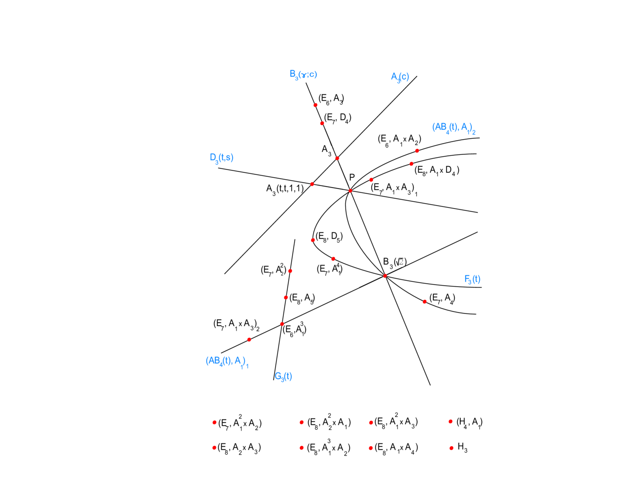
Figure 1: All known $\vee$-systems in dimension 3.

All the curves in the diagram represent one-parameter families of $\vee$-systems except the curves corresponding to $A_{3}-$, $B_{3}-$ and $D_{3}-$families. The families $A_{3}(c)$ and $B_{3}(\gamma;c)$ essentially depend on three parameters (after scalar dilatation of all the vectors in a $\vee$-system) and $D_{3}(t,s)$ is a two-parametric family of $\vee$-systems. The point $P$ on the diagram represents the $\vee$-system $B_{3}(-1;1,1,2)$ which is the intersection of the one-parameter families $(AB_{4}(t),A_{1})_{2}$ and $F_{3}(t)$. Also the point $P$ corresponds to the one-parameter family $B_{3}(-1;1,1,s)$ which is the intersection of $D_{3}-$ and $B_{3}-$ families.

In the diagram we used Theorems 6, 7 and equivalences established in [9]. We also used that in the limit $t\to\infty$ the restrictions of $AB_{4}(t)$-systems are equivalent as follows:

$$(AB_{4}(\infty),A_{1})_{1}=B_{3}(\sqrt{2}),\quad(AB_{4}(\infty),A_{1})_{2}=B_{3}(-1;1,1,2).$$

Acknowledgements. We are grateful to O.A. Chalykh and A.N. Sergeev for useful discussions. The work was partially supported by the European research network ENIGMA (contract MRTN-CT-2004-5652), ESF programme MISGAM and EPSRC (grant EP/E004008/1).

We also acknowledge support of the Isaac Newton Institute for Mathematical Sciences for the hospitality during September 2006, when part of the work was done.

References

- [1] A.P. Veselov Deformations of root systems and new solutions to generalised WDVV equations. Phys. Lett. A 261 (1999), 297.
- [2] A.P. Veselov On geometry of a special class of solutions to generalised WDVV equations. hep-th/0105020. In: Integrability: the Seiberg-Witten and Whitham equations. Ed. by H.W. Braden and I.M. Krichever, Gordon and Breach (2000), 125–135.
- [3] B. Dubrovin Geometry of 2D topological field theories., in: Integrable Systems and Quantum Groups, Montecatini, Terme, 1993. Springer Lecture Notes in Math. 1620 (1996), 120-348.
- [4] A. Marshakov, A. Mironov, and A. Morozov WDVV-like equations in SUSY Yang-Mills theory. Phys.Lett. B, 389 (1996), 43-52.
- [5] B. Dubrovin On almost duality for Frobenius manifolds. math.DG/0307374. In: Geometry, topology, and mathematical physics, AMS Transl. Ser. 2, 212 (2004), 75–132.
- [6] O.A. Chalykh, A.P. Veselov Locus configurations and -systems Phys.Lett.A 285 (2001) 339–349.
- [7] A.P. Veselov On generalizations of the Calogero-Moser-Sutherland quantum problem and WDVV equations. J. Math. Phys. 43 (2002), no. 11, 5675–5682.
- [8] M. Feigin On the logarithmic solutions of the WDVV equations. Czechoslovak J. Phys. 56 (2006), no. 10-11, 1149–1153.
- [9] M.V. Feigin, A.P. Veselov Logarithmic Frobenius structures and Coxeter discriminants, Adv. Math. 212 (2007), no. 1, 143–162.
- [10] A. N. Sergeev, A. P. Veselov Deformed quantum Calogero-Moser systems and Lie superalgebras, Comm. Math. Phys. 245 (2004), 249–278.
- [11] A. Marshakov, A. Mironov, and A. Morozov More evidence for the WDVV equations in N=2 SUSY Yang-Mills theories. Int.J.Mod.Phys. A15 (2000), 1157-1206.
- [12] V. Serganova On generalizations of root systems. Commun. in Algebra 24 (13), (1996), 4281-4299.