Exact ground states for two new spin-1 quantum chains,
new features of matrix product states
         S. Alipour,         V. Karimipour ,         L. Memarzadeh,

Department of Physics, Sharif University of Technology,

P.O. Box 11155-9161, Tehran, Iran

We use the matrix product formalism to find exact ground states of two new spin-$1$ quantum chains with nearest neighbor interactions. One of the models, model I, describes a one-parameter family of quantum chains for which the ground state can be found exactly. In certain limit of the parameter, the Hamiltonian turns into the interesting case $H=\sum_{i}({\bf S}_{i}\cdot{\bf S}_{i+1})^{2}$. The other model which we label as model II, corresponds to a family of solvable three-state vertex models on square lattices. The ground state of this model is highly degenerate and the matrix product states is a generating state of such degenerate states. The simple structure of the matrix product state allows us to determine the properties of degenerate states which are otherwise difficult to determine. For both models we find exact expressions for correlation functions.

PACS Number: 75.10.Jm

1 Introduction

Quantum information theory and condensed matter physics, study many body systems on lattices from complementary points of view. While in condensed matter physics, one starts from a Hamiltonian and seeks to determine the ground state in some approximate form, in quantum information theory the emphasis is on the properties of quantum states, for the quantification of which many tools have been developed in recent years. The subject of Matrix Product States (MPS) lies at the borderline of these two disciplines, since in this formalism, one starts from a quantum many body state with pre-determined properties, and then constructs a family of local Hamiltonians for which this state is an exact ground state. In this way, one may find interesting many-body systems for which the ground state and all its properties, i.e. correlation functions, can be calculated in closed analytical form, a very rare situation which is usually welcomed in condensed matter and statistical physics.

The subject of MPS has a long history in condensed matter physics, the origins of which can be traced back to the work of Majumdar-Ghosh models [1] which in turn inspired the construction of a larger family of solvable spin systems by Affleck, Kennedy, Lieb and Tasaki (AKLT) in [2]. The AKLT construction was further developed in [3, 4] under the name of finitely correlated spin chains or in [5, 6] under the name of optimal ground states. In its simplest version, which applies to translational-invariant systems on rings of $N-$sites, a matrix product state generalizes a product uncorrelated state by replacing numbers by matrices in the following way

$$|\psi\rangle=\sum_{i_{1},i_{2},\cdots i_{N}=1}^{d}tr(A_{i_{1}}A_{i_{2}}\cdots A_{i_{N}})|i_{1},i_{2},\cdots i_{N}\rangle,$$ (1)

where $A_{i}$, $i=1,\cdots d$ are a set of matrices, assigned to the local states $|1\rangle,\cdots|d\rangle$ of a site. The normalization of these states is given by

$$\langle\psi|\psi\rangle=tr(E^{N}),$$ (2)

where $E:=\sum_{i=1}^{d}A_{i}^{*}\otimes A_{i}$. The dimensions of these matrices are arbitrary and are constrained by symmetry considerations and the details of model construction, i.e. the range of interaction. One can collect all the matrices in a vector-valued matrix ${\cal A}$ as follows

$${\cal A}=\sum_{i=1}^{d}A_{i}|i\rangle,$$ (3)

and write the matrix product state (1) as

$$|\psi\rangle=tr({\cal A}\otimes{\cal A}\cdots\otimes{\cal A}),$$ (4)

where the trace is taken over the matrix indices and the tensor product acts on basis vectors, i.e.

$$tr({\cal A}\otimes{\cal B}):=\sum_{i,j}({A_{i}})_{\alpha,\beta}({B_{j}})_{\beta,\alpha}|i,j\rangle.$$

The simple structure of the state (4) allows an exact calculation of correlation functions. For example one and two-point functions of local operators are given by

$$\frac{\langle\psi|O|\psi\rangle}{\langle\psi|\psi\rangle} = \frac{tr(E_{O}E^{N-1})}{tr(E^{N})},$$ (5)

$$\frac{\langle\psi|O_{k}O_{l}|\psi\rangle}{\langle\psi|\psi\rangle} = \frac{tr(E^{k-1}E_{O}E^{l-k-1}E_{O}E^{N-l})}{tr(E^{N})},$$ (6)

where

$$E_{O}=\sum_{i,j}A_{i}^{*}\otimes A_{j}\langle i|O|j\rangle.$$ (7)

In the thermodynamic limit $N\rightarrow\infty$, the right hand sides of the above equations simplify even further, since in this limit, the eigenvalue(s) of $E$ with largest magnitude dominate the traces.

In recent years, this formalism has been used in developing exactly solvable models in spin chains [5, 6, 7, 8, 9, 10, 11], spin ladders [12, 13, 14, 15], spin systems on two dimensional lattices [16, 17, 18], and the study of entanglement properties of spin systems near the points of quantum phase transitions [19, 20, 21, 22]. It has also been used extensively to find the stationary states of many types of stochastic systems of interacting particles in one dimensional chains, see for example [23, 24, 25].

A basic question is then whether we can construct general MPS and its parent Hamiltonians having a set of specific symmetries for quantum chains of spins. For spin-one systems, the first model was given by Affleck, Kennedy, Lieb, and Tasaki in [2], (not within the MPS formalism) which had full rotational symmetry, and was shown later to correspond to the matrix

$${\cal A}_{aklt}=\left(\begin{array}[]{cc}|0\rangle&-\sqrt{2}|1\rangle\\ \sqrt{2}|\overline{1}\rangle&-|0\rangle\end{array}\right),$$ (8)

where $|\overline{1}\rangle=|-1\rangle$ with the parent Hamiltonian

$$H=\sum_{i}{\bf S}_{i}\cdot{\bf S}_{i+1}+\frac{1}{3}({\bf S}_{i}\cdot{\bf S}_{i+1})^{2}.$$ (9)

Then it was shown [5] that if one demands only rotational symmetry around the $z$ axis in spin space, in addition to parity and spin-flip symmetries, a more general model can be constructed which is described by the matrix

$${\cal A}=\left(\begin{array}[]{cc}|0\rangle&-\sqrt{g}|1\rangle\\ \sqrt{g}|\overline{1}\rangle&\sigma|0\rangle\end{array}\right),$$ (10)

where $g$ is a continuous parameter and $\sigma=\pm 1$ is a discrete parameter.

At first sight, construction of a matrix product state, finding its parent Hamiltonian, and calculating the correlation functions, seems a straightforward procedure. However if one demands symmetry properties, and more importantly demands that the final Hamiltonian have a physically interesting interpretation, then the problem will be quite non-trivial and interesting. Specially if one puts the formal MPS under scrutiny, one may be able to find many more states which are not themselves MPS representable, but have been captured by a single MPS in a nice way, i.e. as their generating state. This is what we will find for the models constructed in this paper. We believe that the richness of matrix product formalism has yet to be unraveled by studying more and more examples. In this paper we try to construct two other spin-1 matrix product models, which have not been reported in the literature of matrix product states. The first model is a one-parameter family which has the interesting property to interpolate between two limits, namely between the Ising-like Hamiltonian

$$H_{1}=\sum_{i}(S^{2}_{z,i}-1)(S^{2}_{z,i+1}-1),$$ (11)

and

$$H_{2}=\sum_{i}({\bf S}_{i}\cdot{\bf S}_{i+1})^{2}.$$ (12)

The ground state of (12), as we will see, breaks the rotational symmetry of the Hamiltonian. This is an example of the richness of matrix product formalism, that is by searching the space of solutions, one may come to corners where there are very simple and physically interesting Hamiltonians whose ground states are given by MPS. Clearly the symmetry breaking MPS is not the unique ground state of (12), however the other ground states, can be found by applying the symmetry operators of $su(2)$ group to the MPS.

The other model that we find, labeled as model II, turns out to correspond to a family of solvable three-state vertex models on square lattices, [26, 27]. In this model the degeneracy of the ground states, shows itself in a completely different way, namely, we find that the matrix product depends on a continuous parameter, but the parent Hamiltonian does not, i.e.

$$H|\psi(g)\rangle=E_{0}|\psi(g)\rangle.$$ (13)

Thus if we expand the matrix product state $|\psi(g)\rangle$ in terms of the parameter $g$, in the form

$$|\psi(g)\rangle=\sum_{n=0}^{N}g^{n}|\psi_{n}\rangle,$$ (14)

we obtain a large number of states $|\psi_{n}\rangle$, which all have the same energy and thus represent part of the degenerate ground states of the Hamiltonian. In this way the MPS plays the role of a generating state for a set of degenerate ground states of the Hamiltonian, none of which has a MPS representation. The degree of degeneracy of the ground states increases with system size, and each state $|\psi_{n}\rangle$ has a complicated structure, and can not be represented as a matrix product, and thus the calculation of any of its correlation functions, or even its normalization, is quite difficult. However from the fact that the generating state $|\psi(g)\rangle$ is a matrix product state, we can determine such correlations in closed form.

The structure of this paper is as follows: in section (2) we briefly review the matrix product formalism, with emphasis on the symmetry properties of the state and the parent Hamiltonian, in section (3) we consider three dimensional auxiliary matrices and classify them according to symmetries of the states which are constructed from them, namely symmetry with respect to rotation around the z-axis and the discrete parity and spin-flip symmetries. In this way we arrive at two specific forms of auxiliary matrices and consequently two specific models. Sections (4) and (5) are devoted to the detailed study of the above two models. The paper ends with a conclusion and an appendix.

2 Symmetries of matrix product state and its parent Hamiltonian

From (1) we see that the collections of matrices $\{A_{i}\}$ and $\{\lambda UA_{i}U^{-1}\}$, where $\lambda$ is a scalar, both define the same matrix product state. This freedom allows us to study the symmetries of MPS. A MPS will be symmetric under parity provided that we can find a matrix $\Pi$ such that

$$\Pi A_{m}\Pi^{-1}\propto A_{m}^{T}$$

and invariant under spin flip transformation, if we can find a matrix $\Omega$ such that

$$\Omega A_{m}\Omega^{-1}\propto A_{\overline{m}},$$

where here and hereafter, $A_{\overline{m}}$ stands for $A_{-m}$. As for continuous symmetries, consider a local symmetry operator $R$ acting on a site as $R|i\rangle=R_{ji}|j\rangle$ where summation convention is being used. $R$ is a $d$ dimensional unitary representation of the symmetry. A global symmetry operator ${\cal R}:=R^{\otimes N}$ will then change this state to another matrix product state

$$\Psi_{i_{1}i_{2}\cdots i_{N}}\longrightarrow\Psi^{\prime}:=tr(A^{\prime}_{i_{1}}A^{\prime}_{i_{2}}\cdots A^{\prime}_{i_{N}}),$$ (15)

where

$$A^{\prime}_{i}:=R_{ij}A_{j}.$$ (16)

A sufficient but not necessary condition for the state $|\Psi\rangle$ to be invariant under this symmetry is that there exist an operator $U(R)$ such that

$$R_{ij}A_{j}=U(R)A_{i}U^{-1}(R).$$ (17)

Thus $R$ and $U(R)$ are two unitary representations of the symmetry, respectively of dimensions $d$ and $D$. In case that $R$ is a continuous symmetry operator with generators $T_{a}$, equation (17), leads to

$$(T_{a})_{ij}A_{j}=[{\cal T}_{a},A_{i}],$$ (18)

where $T_{a}$ and ${\cal T}_{a}$ are the $d-$ and $D-$dimensional representations of the Lie algebra of the symmetry.

A symmetric MPS need not be the ground state of a symmetric family of Hamiltonians. To find the symmetric family of Hamiltonians we should construct the Hamiltonian in a specific way. Let us first review how the Hamiltonian is constructed in general. From a matrix product state, the reduced density matrix of $k$ consecutive sites is given by

$$\rho_{i_{1}\cdots i_{k},j_{1}\cdots j_{k}}=\frac{tr((A_{i_{1}}^{*}\cdots A_{i_{k}}^{*}\otimes A_{j_{1}}\cdots A_{j_{k}})E^{N-k})}{tr(E^{N})}.$$ (19)

The null space of this reduced density matrix includes the solutions of the following system of equations

$$\sum_{j_{1},\cdots,j_{k}=1}^{d}c_{j_{1}\cdots j_{k}}A_{j_{1}}\cdots A_{j_{k}}=0.$$ (20)

Given that the matrices $A_{i}$ are of size $D\times D$, there are $D^{2}$ equations with $d^{k}$ unknowns. Since there can be at most $D^{2}$ independent equations, there are at least $d^{k}-D^{2}$ solutions for this system of equations. Thus for the density matrix of $k$ sites to have a null space it is sufficient that the following inequality holds

$$d^{k}\ >\ D^{2}.$$ (21)

Let the null space of the reduced density matrix of $k$ consecutive sites, denoted by ${\cal V}_{k}$, be spanned by the orthogonal vectors $|e_{\alpha}\rangle,\ \ \ (\alpha=1,\cdots,s\geq d^{k}-D^{2})$. Then we can construct the local Hamiltonian acting on $k$ consecutive sites as

$$h:=\sum_{\alpha=1}^{s}J_{\alpha}|e_{\alpha}\rangle\langle e_{\alpha}|,$$ (22)

where $J_{\alpha}$’s are positive constants. These parameters together with the parameters of the vectors $|e_{\alpha}\rangle$ inherited from those of the original matrices $A_{i}$, determine the total number of coupling constants of the Hamiltonian. If we call the embedding of this local Hamiltonian into the sites $l$ to $l+k$ by $h_{l,l+k}$ then the full Hamiltonian on the chain is written as

$$H=\sum_{l=1}^{N}h_{l,l+k}.$$ (23)

The state $|\Psi\rangle$ is then a ground state of this Hamiltonian with vanishing energy. The reason is as follows:

$$\langle\Psi|H|\Psi\rangle=tr(H|\Psi\rangle\langle\Psi|)=\sum_{l=1}^{N}tr(h_{l,l+k}\rho_{l,l+k})=0,$$ (24)

where $\rho_{l,k+l}$ is the reduced density matrix of sites $l$ to $l+k$ and in the last equality we have used the fact that $h$ is constructed from the null eigenvectors of $\rho$ for $k$ consecutive sites. Given that $H$ is a positive operator, this proves the assertion. For the Hamiltonian to have the symmetries of the ground state, the basis vectors of the null space should be chosen so that they transform into each other under the action of symmetries and the couplings $J_{\alpha}$ should be chosen appropriately, see [28] for a more detailed discussion of this point.

3 Three dimensional auxiliary matrices

As is clear from (21) a sufficient condition for the existence of a null space ${\cal V}_{2}$ for a spin-one system is that the dimension of the matrices satisfy $D^{2}<9$ which restricts $D$ to $1$ and $2$. The case of $D=1$ has already been considered in [29] outside the framework of MPS formalism, and the case of $D=2$ has been worked out in [2] and [5] as mentioned in the introduction. However we should emphasize that this is a sufficient and not a necessary condition and indeed we can take $D\geq 3$ and still find a non-empty null space ${\cal V}_{2}$, since the system of equations may not all be independent of each other.

In this article we want to study in detail the case $D=3$ and consider all the possible models which allow certain plausible symmetries, i.e. rotational symmetry around the $z$ axis in spin space, and symmetry under parity and spin flip operations, these are the symmetries which have been taken into account in building optimal ground states for various models [4, 5, 6, 7, 8, 12, 16, 17, 22].

So let us take 3-dimensional matrices $A_{1},A_{0}$ and $A_{\overline{1}}$ and demand rotational symmetry around the $z$ axis in spin space. According to (18), this is equivalent to the following equations

$$[S_{z},A_{1}]=A_{1},\hskip 28.45274pt[S_{z},A_{0}]=0,\hskip 28.45274pt[S_{z},A_{\overline{1}}]=-A_{\overline{1}},$$ (25)

where $S_{z}=diagonal(1,0,-1)$. The immediate solution of these equations is

$$A_{1}=\left(\begin{array}[]{c c c}0&a&0\\ 0&0&b\\ 0&0&0\end{array}\right)\hskip 28.45274ptA_{0}=\left(\begin{array}[]{c c c}g&0&0\\ 0&h&0\\ 0&0&i\end{array}\right)\hskip 28.45274ptA_{\overline{1}}=\left(\begin{array}[]{c c c}0&0&0\\ c&0&0\\ 0&d&0\end{array}\right),$$ (26)

where $a,b,c,d,g,h$ and $i$ are real parameters. By a transformation $A_{i}\longrightarrow SA_{i}S^{-1}$ where $S=diagonal(1,a,ab)$ we can set the parameters of $A_{1}$ equal to 1. Symmetry under parity now requires that there is a matrix $\Pi$ such that

$$\Pi A_{m}\Pi^{-1}=A^{T}_{m}.$$ (27)

A straightforward calculation gives

$$\Pi=\left(\begin{array}[]{ccc}0&0&1\\ 0&1&0\\ 1&0&0\end{array}\right)$$ (28)

and

$$A_{1}=\left(\begin{array}[]{ccc}0&1&0\\ 0&0&1\\ 0&0&0\end{array}\right),\ \ \ A_{0}=\left(\begin{array}[]{ccc}g&0&0\\ 0&h&0\\ 0&0&g\end{array}\right),\ \ \ A_{\overline{1}}=\left(\begin{array}[]{ccc}0&0&0\\ c&0&0\\ 0&c&0\end{array}\right).$$ (29)

Finally we come to the symmetry under spin flip $|m\rangle\longrightarrow|\overline{m}\rangle$. It is readily seen that with these matrices the spin-flip symmetry is automatic, namely we have

$$\Omega A_{m}\Omega^{-1}=A_{\overline{m}},$$ (30)

in which

$$\Omega=\left(\begin{array}[]{ccc}0&0&1\\ 0&{c}&0\\ {c^{2}}&0&0\end{array}\right).$$ (31)

In order to guarantee that the matrix product state constructed in this way is the ground state of a Hamiltonian with nearest neighbor interaction, we consider the equation

$$\sum_{i,j=1,0,\overline{1}}c_{ij}A_{i}A_{j}=0,$$ (32)

which can be re-written as a matrix equation for the coefficients $c_{ij}$ in the form

$$\sum_{i,j}M_{kl,ij}c_{ij}=0.$$ (33)

To have a solution we set

$$det(M)=0.$$ (34)

The determinant of $M$ is readily calculated from its explicit form and is given by

$$det(M)=(g^{2}-h^{2})^{2}(2g^{2}-h^{2})c^{4}.$$ (35)

The vanishing of the determinant puts constrains on the parameters, namely we should have either $c=0$, or $h=\pm g$ or $h=\pm\sqrt{2}g$, each choice leading to a different exactly solvable model. We omit the case $c=0$ since it leads to the condition $A_{\overline{1}}=0$ and hence reduces the model to an effectively two-state model, moreover in this case, spin-flip symmetry is lost due to the non-existence of an invertible matrix $\Omega$. Also it turns out that the other models with minus signs are equivalent to models with plus signs, see appendix A for a demonstration of this fact. So we are left with two different models which we label accordingly as model I (when $h=\sqrt{2}g$) and model II (when $h=g$) and study them separately in subsequent sections.

Before proceeding to the models, we need to clarify a point about the number of parameters. Throughout our analysis we take $N$, the size of the lattice to be an even number. It appears that we have two continuous parameters in the matrix product states, namely $g$ and $c$. None of these parameters can be gauged away by similarity transformations or scaling of the auxiliary matrices. However the MPS depends on only one parameter. To see this, let us expand the MPS in terms of the states $|\psi_{n}\rangle$ which are defined to be linear superposition of all states which have $n$ $0$’s. Note that for an even $N$, $n$ will also have to be even. Since in the space of one site, the operators $A_{1}$ and $A_{\overline{1}}$ act as raising and lowering operators, the trace of any string of operators $A_{0},A_{1}$ and $A_{\overline{1}}$ is non-vanishing only if this string contains an equal number of $A_{1}$ and $A_{\overline{1}}$. Thus any state $|\psi_{n}\rangle$ comes with a coefficient $g^{n}c^{\frac{N-n}{2}}$. Consequently for the un-normalized MPS we have

$$|\psi(g,c)\rangle=\sum_{n=0}^{N}g^{n}c^{\frac{N-n}{2}}|\psi_{n}\rangle\equiv c^{\frac{N}{2}}\sum_{n=0}^{N}(\frac{g^{2}}{c})^{\frac{n}{2}}|\psi_{n}\rangle.$$ (36)

Thus the normalized state and all the correlation functions will depend on only one single parameter, namely $\frac{g^{2}}{c}$. For this reason we can put $c=1$ and so the MPS will depend on only one single parameter $g$.

4 Model I

In this section we study in detail model I. The auxiliary matrices are

$$A_{1}=\left(\begin{array}[]{ccc}0&1&0\\ 0&0&1\\ 0&0&0\end{array}\right),\ \ \ A_{0}=g\left(\begin{array}[]{ccc}1&0&0\\ 0&\sqrt{2}&0\\ 0&0&1\end{array}\right),\ \ \ A_{\overline{1}}=\left(\begin{array}[]{ccc}0&0&0\\ 1&0&0\\ 0&1&0\end{array}\right).$$ (37)

First we derive the one-parameter family of parent Hamiltonians and then calculate the one and the two-point functions.

4.1 The Hamiltonian

Here we have $h=\sqrt{2}g$ and the null space ${\cal V}_{2}$ is spanned by one single vector

$$|e\rangle=|00\rangle-g^{2}|1,\overline{1}\rangle-g^{2}|\overline{1},1\rangle.$$ (38)

We take the local Hamiltonian as $h_{I}=\frac{1}{(1-g^{2})^{2}}|e\rangle\langle e|$ from which the full Hamiltonian turns out to be

$$H_{I}(u)=(1-u^{2})N+\sum_{i}S_{z,i}^{2}S_{z,i+1}^{2}-2(1+2u)S_{z,i}^{2}+u^{2}({\bf S}_{i}\cdot{\bf S}_{i+1})^{2}+u\{{\bf S}_{i}\cdot{\bf S}_{i+1},S_{z,i}S_{z,i+1}\},$$ (39)

where $u:=\frac{g^{2}}{1-g^{2}}$. When $g=u=0$, the Hamiltonian turns into

$$H_{1}=\sum_{i}(S^{2}_{z,i}-1)(S^{2}_{z,i+1}-1).$$ (40)

In this limit, since $A_{0}\rightarrow 0$, the MPS becomes an expansion of states consisting only of $1$ and $\overline{1}$. Such a state is clearly the ground state of the Hamiltonian (40), however, the Hamiltonian (40) has a highly degenerate ground state, which is not captured by the MPS in this limit. In fact, any basis state in which no two $0$’s are adjacent is a ground state of this Hamiltonian, with energy $E_{0}=0$. The number of ground states of $H_{1}$ is equal to $tr(A^{N})$, where $N$ is the system size and $A$ is the adjacency matrix in which allowed adjacent configurations are designated by $1$ and disallowed configurations by $0$. In $H_{1}$ the only configuration which lifts the local energy from $0$ to $1$ is that of two adjacent zeros, so in the basis which we have chosen, $A=\left(\begin{array}[]{ccc}1&1&1\\ 1&0&1\\ 1&1&1\end{array}\right)$. For large $N$, we will have $tr(A)^{N}\approx(1+\sqrt{3})^{N}$, where $1+\sqrt{3}$ denote the largest eigenvalue of $A$.

When $g\rightarrow 1$ (or $u\rightarrow\infty$), $H_{I}(u)$ turns, modulo a multiplicative coefficient, into the following Hamiltonian,

$$H_{2}=\sum_{i}[({\bf S}_{i}\cdot{\bf S}_{i+1})^{2}-1].$$ (41)

This is a simple and interesting Hamiltonian and thus our result implies that its ground state is of the form of an MPS, with matrices given by (37), for $g=1$.

Note that in the limit $g=1$, the null eigenvector (38) becomes a singlet, the spin-0 representation of angular momentum, implying that the Hamiltonian should be a scalar which conforms with the form of the Hamiltonian (41). However the matrices (37) (for $g=1$) do not transform as a spherical tensor operator under angular momentum, that is the following relations are not satisfied as required from (18):

$$[S_{z},A_{m}] = mA_{m}$$ (42)

$$[S_{+},A_{m}] = \sqrt{2-m(m+1)}A_{m+1}$$ (43)

$$[S_{-},A_{m}] = \sqrt{2-m(m-1)}A_{m-1},$$ (44)

where $S_{z}$, and $S_{\pm}$ are the three dimensional representation of $su(2)$. This means that the Hamiltonian is symmetric under the full rotation group, but the ground state, breaks this symmetry. Therefore other degenerate ground states can be constructed by applying rotation operators to this state. However the actual degeneracy is much larger and it grows exponentially with system size as $(\frac{3+\sqrt{5}}{2})^{N}$ [30].

We should stress that the Hamiltonian $H_{2}$ corresponds to a particular point in the class of bilinear-biquadratic spin-1 chains with the Hamiltonian

$$H(\theta):=\sum_{i=1}^{N}\left[\cos\theta\ {\bf S}_{i}\cdot{\bf S}_{i+1}+\sin\theta\ ({\bf S}_{i}\cdot{\bf S}_{i+1})^{2}\right]$$ (45)

which has extensively been studied by various methods [31, 32, 33, 34, 35, 36].

4.2 Correlation functions

The correlation functions of this model are determined after lengthy but straightforward calculations starting from (5) and (7). In the thermodynamic limit, the results are as follows:

$$\langle S_{z,i}\rangle=\langle S_{x,i}\rangle=0.$$ (46)

Thus in the ground state, there is no magnetization. Note that due to rotational invariance in the $x-y$ plane of spin space, in all the correlation functions below, we can change $x$ to $y$ or any other direction in the $x-y$ plane. To describe the other correlation functions, let us introduce the parameter $\gamma:=\sqrt{g^{4}+8}$. Then we have

$$\langle S^{2}_{z,i}\rangle=\frac{8}{\gamma(3g^{2}+\gamma)},\hskip 28.45274pt\langle S^{2}_{x,i}\rangle=\frac{g^{2}(3\gamma+g^{2})+4}{\gamma(3g^{2}+\gamma)}.$$ (47)

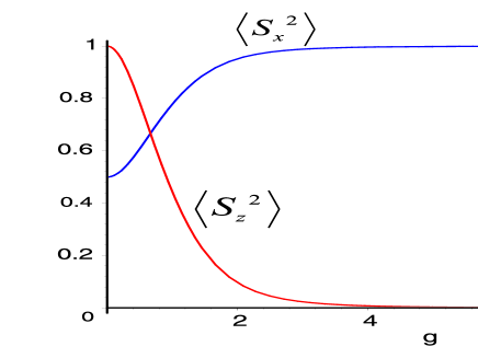
Figure 1: The average values $\langle S_{z}^{2}\rangle$ and $\langle S_{x}^{2}\rangle$ for model I. In the limit $g\rightarrow\infty(u\rightarrow-1)$

, the spins lie in the $x-y$ plane.

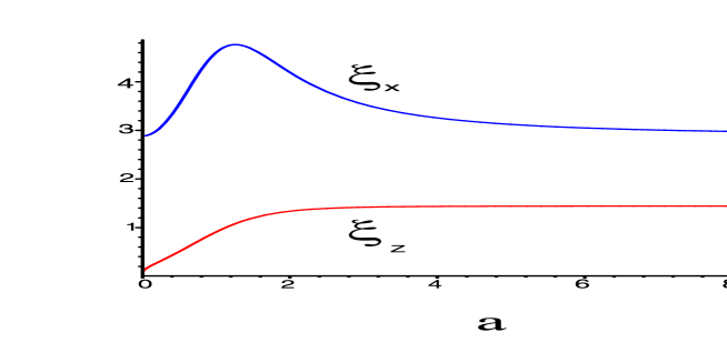
Figure 2: The correlation functions for longitudinal and transverse components of spins, in model I; a) Correlation lengths, b) the magnitudes of correlations.

Figure (1) shows the plot of $\langle S^{2}_{z,i}\rangle$ and $\langle S^{2}_{x,i}\rangle$ as a function of the parameter $g$. In the limit $g\rightarrow 0$, we have $\langle S^{2}_{z,i}\rangle\rightarrow 1$, implying that there is no $0$ in the expansion of the state. This is in accord with our picture of the MPS, since in this limit $A_{0}\rightarrow 0$. Finally for the two point correlations of longitudinal and transverse components of spins we find

$$\langle S_{z,1}S_{z,r}\rangle = G_{||}(g)\ e^{-(r-2)/\xi_{||}},$$ (48)

$$\langle S_{x,1}S_{x,r}\rangle = G_{\perp}(g)\ e^{-(r-2)/\xi_{\perp}},$$ (49)

where the magnitude of correlations are given by

$$G_{||}(g)=-\frac{4(g^{2}+\gamma)}{\gamma(3g^{2}+\gamma)^{2}},\hskip 28.45274ptG_{\perp}(g)=\frac{8g^{2}(g^{2}+\sqrt{2}+\gamma)^{2}}{\gamma(3g^{2}+\gamma)^{2}(g^{2}+\gamma)},$$ (50)

and the longitudinal and transverse correlations are given by

$$\xi_{||}=\frac{1}{\ln(\frac{3g^{2}+\gamma}{2g^{2}})},\hskip 28.45274pt\xi_{\perp}=\frac{1}{\ln(\frac{3g^{2}+\gamma}{2+2\sqrt{2}g^{2}})}.$$ (51)

These are plotted in figure (2). Note that $G_{||}(g)=\langle S_{z,1}S_{z,2}\rangle$ and $G_{\perp}(g)=\langle S_{x,1}S_{x,2}\rangle$. In the limit $g\longrightarrow 0$, where $H_{I}$ becomes an Ising-like Hamiltonian, the above equations show that transverse correlations vanish, and longitudinal correlations approach the value $-1/2$. However we should note that in this limit, the ground state is highly degenerate. In fact as stated above, any basis state in which there are no two adjacent $0$’s is a ground state of $H_{1}$. However the MPS does not capture this degeneracy, but is only one of the many ground states. In the limit $g\rightarrow 1$, where the Hamiltonian turns into (41), we have $\langle S^{2}_{z,i}\rangle=\frac{4}{9}$ and $\langle S^{2}_{x,i}\rangle=\frac{7}{9}$, and the correlation lengths tend to $\xi_{||}=\frac{1}{\ln(3)}=0.910$ and $\xi_{\perp}=\frac{1}{\ln(3/(1+\sqrt{2}))}=4.603$.

5 Model II

For this model, the auxiliary matrices are

$$A_{1}=\left(\begin{array}[]{ccc}0&1&0\\ 0&0&1\\ 0&0&0\end{array}\right),\ \ \ A_{0}=g\left(\begin{array}[]{ccc}1&0&0\\ 0&1&0\\ 0&0&1\end{array}\right),\ \ \ A_{\overline{1}}=\left(\begin{array}[]{ccc}0&0&0\\ 1&0&0\\ 0&1&0\end{array}\right).$$ (52)

5.1 The Hamiltonian

The null space ${\cal V}_{2}$ is spanned by the following two vectors:

$$|e_{1}\rangle=\frac{1}{\sqrt{2}}(|01\rangle-|10\rangle),$$ (53)

$$|e_{2}\rangle=\frac{1}{\sqrt{2}}(|0\overline{1}\rangle-|\overline{1}0\rangle).$$ (54)

These vectors are eigenvectors of the local two-site $S_{z}$ operator, are invariant under parity and transform into each other under spin flip transformation. Therefore if we take the local symmetric Hamiltonian as

$$h_{II}=|e_{1}\rangle\langle e_{1}|+|e_{2}\rangle\langle e_{2}|,$$ (55)

where we have set a total multiplicative constant equal to unity, the final total Hamiltonian is spin-flip and parity invariant and moreover commutes with the third component of spin, i.e. $[h_{II},S_{z}]=0$. Its explicit form in terms of local spin operators can be determined after some algebra:

$$H_{II}=\sum_{i=1}^{N}2S^{2}_{z,i}-\{{\bf S}_{i}.{\bf S}_{i+1},S_{z,i}S_{z,i+1}\}-{\bf S}_{i}.{\bf S}_{i+1}+S_{z,i}S_{z,i+1}.$$ (56)

This Hamiltonian was first found in [27]. The history is the following: The exhaustive solutions of the Yang-Baxter equation, corresponding to a three-state 19-vertex model on a square lattice were first found in [26]. These solutions reproduced many of the already known exactly solvable vertex models in addition to four new models. These models, labeled I, II, III and IV in [27], were then studied in detail in [27], where the thermodynamic properties of these new models, including the partition function and correlation lengths were derived. Two of these models, namely models I and II, however allowed a more complete solution (due to the so called crossing symmetry of the $R$ matrix, the solution of the Yang-Baxter equation) which allowed the exact determination of the ground state energy per site. However the other two models, models III and IV, lacked this symmetry, and no exact solution for the ground state energy was given. It could however be established that such models can be mapped to 6-vertex models, i.e. two state models with 6 allowed configurations. The Hamiltonian (56) corresponds in fact to the Hamiltonian of model III in [27], for $\Delta=1$, where $\Delta$ is a particular combination of Boltzmann weights. For its definition and the Boltzmann weights see [27]. According to [27], the three-state 19-vertex model corresponding to this spin chain is defined by the Boltzmann weights shown in figure (3).

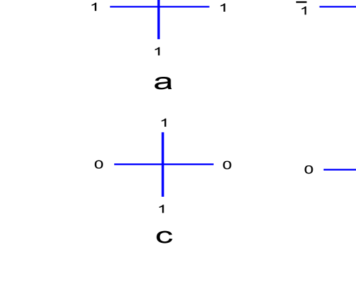
Figure 3: The independent Boltzmann weights of the two dimensinal vertex model corresponding to the quantum spin chain (56).

Note that each Boltzmann weight $R^{\mu,\alpha}_{\nu,\beta}$ corresponds to the spin labels, $\mu,\nu,\alpha,\beta$ on left, right, bottom and top links of a vertex and the $R$ matrix and correspondingly the Boltzmann weights have the following symmetries (with $\overline{\alpha}:=-\alpha,etc):$

$$R^{\mu,\alpha}_{\nu,\beta}=R^{\alpha,\mu}_{\beta,\nu}=R^{\nu,\beta}_{\mu,\alpha}=R^{\overline{\mu},\overline{\alpha}}_{\overline{\nu},\overline{\beta}}.$$ (57)

The exact correspondence between the Hamiltonian (56) and that of model III of [27] is as follows:

$$H_{II}=H_{6-{\rm vertex}}+N,$$ (58)

where $N$ is the number of sites of the chain. This correspondence allows to determine exactly the ground state energy of the corresponding 6-vertex model, for the range of values of Boltzmann weights of the 6-vertex model shown in figure (3). Since the ground state energy of $H$ is zero, we find the ground state energy of $H_{6-{\rm vertex}}$ to be $E_{0}=-N$, giving an energy per site equal to $e_{0}:=\frac{E_{0}}{N}=-1$.

5.2 The explicit form of the ground states

From the form of the local Hamiltonian one finds that any state which comprises of only $1$’s and $\overline{1}$’s, with no $0$’s, is a ground state of this Hamiltonian. The number of such states is $2^{N}$, where $N$ is the size of the system and their explicit form is $|s_{1},s_{2},\cdots s_{N}\rangle$, where $s_{i}\in\{1,\overline{1}\}$. However there are other non-trivial ground states, those which contain also a number of $0$’s. The interesting point is that these kinds of ground states, are nicely captured by the MPS (52). We can find $N$ such degenerate states. To see this we note that MPS (52) depends on a continuous parameter $g$ while the Hamiltonian does not. This dependence is genuine and can not be gauged away by similarity transformation $A_{m}\longrightarrow UA_{m}U^{-1}$. Let us expand the MPS in terms of powers of $g$ in the form

$$|\psi(g)\rangle=\sum_{n=0}^{N}g^{n}|\psi_{n}\rangle,$$ (59)

where

$$|\psi_{n}\rangle=\sum^{\prime}_{i_{1},i_{2},\cdots i_{N}}tr(A_{i_{1}}A_{i_{2}}\cdots A_{i_{N}})|i_{1},i_{2},\cdots i_{N}\rangle,$$ (60)

and $\sum^{\prime}$ implies that in each term only $n$ $A_{0}$’s exist.

In view of (52) and the definition of MPS (4) the powers of $g$ enumerate the number of $0$’s in each state and so each $|\psi_{n}\rangle$ is a superposition of states each of which has exactly $n$ local $0$’s and an equal number of $1$’s and $\overline{1}$’s. Note that since we have taken $N$ to be even, this implies that $n$ is also an even number.

To determine the explicit form of each state $|\psi_{n}\rangle$, consider the form of the matrices $A_{0},A_{1}$ and $A_{\overline{1}}$ in (52). With

$$|1\rangle:=\left(\begin{array}[]{c}1\\ 0\\ 0\end{array}\right),\hskip 28.45274pt|0\rangle:=\left(\begin{array}[]{c}0\\ 1\\ 0\end{array}\right)\hskip 28.45274pt|\overline{1}\rangle:=\left(\begin{array}[]{c}0\\ 0\\ 1\end{array}\right),$$

we have

$$A_{1}=|1\rangle\langle 0|+|0\rangle\langle\overline{1}|,\hskip 28.45274ptA_{0}=gI,\hskip 28.45274ptA_{\overline{1}}=|\overline{1}\rangle\langle 0|+|0\rangle\langle 1|,$$ (61)

or more compactly

$$A_{m}=|m\rangle\langle 0|+|0\rangle\langle\overline{m}|,\hskip 28.45274ptA_{0}=gI,$$ (62)

where $m=1,\overline{1}$ and $I$ is the identity matrix. The product of any string of matrices $A_{m}$, $m=1,\overline{1}$ has a simple structure. One can easily show that

$$A_{m_{1}}A_{m_{2}}\cdots A_{m_{2K}} = \delta_{m_{1},\overline{m_{2}}}\delta_{m_{3},\overline{m_{4}}}\cdots\delta_{m_{2K-1},\overline{m_{2K}}}|0\rangle\langle 0|$$ (63)

$$+ \delta_{\overline{m_{2}},m_{3}}\delta_{\overline{m_{4}},m_{5}}\cdots\delta_{\overline{m_{2K-2}},m_{2K-1}}|m_{1}\rangle\langle\overline{m_{2k}}|.$$ (64)

This allows us to determine the explicit form of any of the states $|\psi_{n}\rangle$. Consider for example $|\psi_{N}\rangle$, where there is no $1$ or $\overline{1}$. This is a simple state $|\psi_{N}\rangle=3|0,0,\cdots 0\rangle$, where the factor $3$ comes from taking the trace of the identity matrix, related to the product of all the $A_{0}$ matrices. The next state is $|\psi_{N-2}\rangle$ in which two of the zeros have been replaces by $1$ and $\overline{1}$. Using (63) we find that this is a state of the form

$$|\psi_{N-2}\rangle=2\sum_{m<n}(|0,\cdots 0,1_{m},0,\cdots,0,\overline{1}_{n},0,\cdots 0\rangle+|0,\cdots 0,\overline{1}_{m},0,\cdots,0,1_{n},0,\cdots 0\rangle),$$ (65)

where the two non-zero spins occur at sites $m$ and $n$ respectively. Let us define $|\alpha_{ij}\rangle:=|1_{i},\overline{1}_{j}\rangle+|\overline{1}_{i},1_{j}\rangle$ where the indices denote the sites of the lattice, and all other sites are occupied by $0$. Then $|\psi_{N-2}\rangle=2\sum_{i<j}|\alpha_{ij}\rangle$. In view of (63), we find the structure of all other states $|\psi_{n}\rangle$. For example we have

$$|\psi_{N-4}\rangle=\sum_{i<j<k<l}(|\alpha_{ij}\rangle|\alpha_{kl}\rangle+|\alpha_{jk}\alpha_{li}\rangle,$$ (66)

which is pictorially depicted in figure (4) and

$$|\psi_{N-6}\rangle=\sum_{i<j<k<l<m<n}\left(|\alpha\rangle_{ij}|\alpha\rangle_{kl}|\alpha\rangle_{mn}+|\alpha\rangle_{ni}|\alpha\rangle_{jk}|\alpha\rangle_{lm}\right).$$ (67)

Finally we find $\psi_{0}$, in which there are no zeros, and has a dimmerized or Majumdar-Ghosh like structure, namely

$$|\psi_{0}\rangle=|\alpha_{12}\rangle|\alpha_{34}\rangle\cdots|\alpha_{N-1,N}\rangle+|\alpha_{23}\rangle|\alpha_{45}\rangle\cdots|\alpha_{N,1}\rangle,$$ (68)

which is depicted in figure (5).

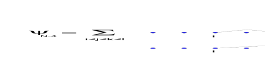
Figure 4: The state $|\psi_{N-4}\rangle$. All the dots are at the state $|0\rangle$, while those which are connected are at the state $|1,\overline{1}\rangle+|\overline{1},1\rangle$.

5.3 Correlation functions

We have found that the number of degenerate ground states of model II, for a chain of size $N$, is at least $2^{N}+N$. Of these, the $2^{N}$ states $|s_{1},s_{2},\cdots s_{N}\rangle$, where $s_{i}\in\{1,\overline{1}\}$ are uncorrelated, even for finite-size systems. The other $N$ states are non-trivial and have MP representations. Here we calculate the correlation functions for the other types of states which are correlated. Were it not for the matrix product formalism, such calculation could be very difficult. As a first step let us determine the normalization of the states $|\psi_{n}\rangle$, and then proceed to the calculation of correlation functions of various operators.

Figure 5: The state $|\psi_{0}\rangle$ has a Majumdar-Ghosh like structure. Note that a line here means only an entangled state $|1,\overline{1}\rangle+|\overline{1},1\rangle$ and not a spin singlet.

Let us first fix our notation for matrix product operators, using their general definition (7). We have

$$E_{S_{z}} = A_{1}\otimes A_{1}-A_{\overline{1}}\otimes A_{\overline{1}}=:U,$$ (69)

$$E_{S_{z}^{2}} = A_{1}\otimes A_{1}+A_{\overline{1}}\otimes A_{\overline{1}}=V,$$ (70)

$$E\ = A_{1}\otimes A_{1}+A_{\overline{1}}\otimes A_{\overline{1}}+A_{0}\otimes A_{0}=V+g^{2}I.$$ (71)

Let us start by finding the normalization of the states $|\psi_{n}\rangle$. It is obvious that for $m\neq n$, $\langle\psi_{m}|\psi_{n}\rangle=0,$ since these two states, have different number of zeros in their expansion. Therefore

$$\langle\psi(g)|\psi(g)\rangle=\sum_{n=0}^{N}g^{2n}\langle\psi_{n}|\psi_{n}\rangle.$$ (72)

The left hand side is found from (2) to be

$$\langle\psi(g)|\psi(g)\rangle=tr(E^{N})=tr(V+g^{2}I)^{N}=\sum_{n=0}^{N}g^{2n}\left(\begin{array}[]{c}N\\ n\end{array}\right)tr(V^{N-n}).$$

Comparing with the previous formula, we find

$$\langle\psi_{n}|\psi_{n}\rangle=\left(\begin{array}[]{c}N\\ n\end{array}\right)tr(V^{N-n}).$$ (73)

5.3.1 One-point functions

In the thermodynamic limit $N\longrightarrow\infty$ (n=finite), the traces are simplified by taking only the largest eigenvalues, but before going to this limit, let us derive closed formulas for some of the correlation functions. From the nature of the states $|\psi_{n}\rangle,$ it is obvious that

$$\langle\psi_{n}|S_{z}|\psi_{n}\rangle=\langle\psi_{n}|S_{a}|\psi_{n}\rangle=0,$$ (74)

where $a$ is any direction perpendicular to the $z$ axis. To obtain the average of $S_{z}^{2}$, we note again that for $m\neq n$, $\langle\psi_{n}|S_{z}^{2}|\psi_{m}\rangle=0$ and hence

$$\langle\psi(g)|S_{z}^{2}|\psi(g)\rangle=\sum_{n=0}^{N}g^{2n}\langle\psi_{n}|S_{z}^{2}|\psi_{n}\rangle.$$ (75)

The left hand side is obtained from (5):

$$\langle\psi(g)|S_{z}^{2}|\psi(g)\rangle=tr(E_{S^{2}_{z}}E^{N-1})=tr(V(V+g^{2}I)^{N-1})=\sum_{n=0}^{N-1}g^{2n}\left(\begin{array}[]{c}N-1\\ n\end{array}\right)tr(V^{N-n}),$$ (76)

which in view of (75) gives

$$\frac{\langle\psi_{n}|S_{z}^{2}|\psi_{n}\rangle}{\langle\psi_{n}|\psi_{n}\rangle}=\frac{\left(\begin{array}[]{c}N-1\\ n\end{array}\right)}{\left(\begin{array}[]{c}N\\ n\end{array}\right)}=\frac{N-n}{N},$$ (77)

as expected, since the operator $S_{z}^{2}$ counts the average number of $1$’s or $\overline{1}$’s in the state. From $\langle S_{x}^{2}+S_{y}^{2}+S_{z}^{2}\rangle=2$ and the rotational symmetry around the $z$ axis, we find for any unit vector $a$ in the $x-y$ plane

$$\frac{\langle\psi_{n}|S_{a}^{2}|\psi_{n}\rangle}{\langle\psi_{n}|\psi_{n}\rangle}=\frac{N+n}{2N}.$$ (78)

5.3.2 Two-point functions

Let us now derive the two point correlation functions, $\langle\psi_{n}|S_{z,1}S_{z,r}|\psi_{n}\rangle$. We have

$$\langle\psi(g)|S_{z,1}S_{z,r}|\psi(g)\rangle=tr(E_{S_{z}}E^{r-2}E_{S_{z}}E^{N-r})=tr(U(V+g^{2}I)^{r-2}U(V+g^{2}I)^{N-r})$$

Expanding the right hand side and using the diagonal property of this two-point function, namely that for $m\neq n$, $\langle\psi_{n}|S_{z,1}S_{z,r}|\psi_{m}\rangle=0,$ we find

$$\frac{\langle\psi_{n}|S_{z,1}S_{z,r}|\psi_{n}\rangle}{\langle\psi_{n}|\psi_{n}\rangle}=\frac{\sum_{k=0}^{r-2}\left(\begin{array}[]{c}r-2\\ k\end{array}\right)\left(\begin{array}[]{c}N-r\\ n-k\end{array}\right)tr(UV^{r-2-k}UV^{N-r-n+k})}{\left(\begin{array}[]{c}N\\ n\end{array}\right)tr(V^{N-n})}.$$ (79)

The expansion of $\langle\psi(g)|S^{2}_{z,1}S^{2}_{z,r}|\psi(g)\rangle$ gives a simple result, since in this case, the matrix product operator $E_{S^{2}_{z}}=V$ commutes with $E$, that is

$$\langle\psi(g)|S^{2}_{z,1}S^{2}_{z,r}|\psi(g)\rangle = tr(V(V+g^{2}I)^{r-2}V(V+g^{2}I)^{N-r})=tr(V^{2}(V+g^{2}I)^{N-2})$$ (80)

$$= \sum_{n=0}^{N-2}\left(\begin{array}[]{c}N-2\\ n\end{array}\right)g^{2n}tr(V^{N-n}),$$ (83)

giving the final distance-independent result

$$\frac{\langle\psi_{n}|S^{2}_{z,1}S^{2}_{z,r}|\psi_{n}\rangle}{\langle\psi_{n}|\psi_{n}\rangle}=\frac{\left(\begin{array}[]{c}N-2\\ n\end{array}\right)}{\left(\begin{array}[]{c}N\\ n\end{array}\right)}=\frac{(N-n)(N-n-1)}{N(N-1)}.$$ (84)

Finally we come to the two-point function $\langle S_{x,1}S_{x,r}\rangle$ between transverse components of spins. Here we encounter an essential difference with the previous cases, in that the operator $S_{x}$ is not diagonal between the states $|\psi_{n}\rangle$, i.e. $\langle\psi_{n}|S_{x,1}S_{x,r}|\psi_{m}\rangle\neq 0$ for $m\neq 0$. To circumvent this problem, we do the following expansion, for $g$ and $h$ two arbitrary variables:

$$\langle\psi(g)|S_{x,1}S_{x,r}|\psi(h)\rangle=\sum_{n,m=0}^{N}g^{n}h^{m}\langle\psi_{n}|S_{x,1}S_{x,r}|\psi_{m}\rangle.$$ (85)

To calculate the left hand side within the matrix product formalism, we should slightly adapt equations (2), (5) and (7) to conform to the present situation. Let $|\phi\rangle$ and $|\psi\rangle$ be two matrix product states on the same periodic lattice of size $N$, defined by matrices $\{A_{i}\}$ and $\{B_{i}\}$ respectively. Then by following the steps which led to (2) and (5) we find

$$\langle\phi|\psi\rangle=tr(\tilde{E}^{N}),$$ (86)

where $\tilde{E}=\sum_{i}A_{i}^{*}\otimes B_{i}$. The one point function of an observable $O$ will be given by

$$\langle\phi|O|\psi\rangle=tr(\tilde{E}_{O}\tilde{E}^{N-1}),$$ (87)

where

$$\tilde{E}_{O}=\sum_{i,j}A_{i}^{*}\otimes B_{j}\langle i|O|j\rangle.$$ (88)

We now use the above formulas to calculate the left hand side of (85), where $|\psi(g)\rangle$ and $|\psi(h)\rangle$ are both matrix product states with matrices $A_{i}(g)$ and $A_{i}(h)$ respectively. For the operator in question, namely $S_{x}$, we find from

$$S_{x}=\frac{1}{\sqrt{2}}(|0\rangle\langle 1|+|0\rangle\langle\overline{1}|+|1\rangle\langle 0|+|\overline{1}\rangle\langle 0|)$$

the form of its matrix operator,

$$\tilde{E}_{S_{x}}=\frac{1}{\sqrt{2}}(gI\otimes(A_{1}+A_{\overline{1}})+(A_{1}+A_{\overline{1}})\otimes hI),$$ (89)

which can be simply written as

$$\tilde{E}_{S_{x}}=\frac{1}{\sqrt{2}}(gX_{2}+hX_{1}),$$ (90)

where $X=A_{1}+A_{\overline{1}}$ and the indices on $X$ means its embedding on the first and second spaces. Thus we obtain

$$\langle\psi(g)|S_{x,1}S_{x,r}|\psi(h)\rangle=\frac{1}{2}tr((gX_{2}+hX_{1})(V+ghI)^{r-2}(gX_{2}+hX_{1})(V+gh)^{N-r-2}).$$ (91)

Expanding the right hand side and collecting the coefficient of $(gh)^{n}$ will give

$$\frac{\langle\psi_{n}|S_{x,1}S_{x,r}|\psi_{n}\rangle}{\langle\psi_{n}|\psi_{n}\rangle}=\frac{1}{2}\frac{\sum_{k=0}^{r-2}\left(\begin{array}[]{c}r-2\\ k\end{array}\right)\left(\begin{array}[]{c}N-r-2\\ n-1-k\end{array}\right)tr(\Omega^{x}_{N,r,k,n})}{\left(\begin{array}[]{c}N\\ n\end{array}\right)tr(V^{N-n})},$$ (92)

where

$$\Omega^{x}_{N,r,k,n}:=X_{2}V^{r-2-k}X_{1}V^{N-r-n-1+k}+X_{1}V^{r-2-k}X_{2}V^{N-r-n-1+k}$$ (93)

We now come to the thermodynamic limit of these correlation functions.

5.3.3 The thermodynamic limit

In this subsection we calculate the thermodynamic limit of the correlation functions found above, by which we mean taking $N\longrightarrow\infty$ while keeping $r$ and $n$ fixed. In this limit, the sums in the numerators of equations (79) or (92) are dominated by their $k=0$ term, therefore we find from (79)

$$\frac{\langle\psi_{n}|S_{z,1}S_{z,r}|\psi_{n}\rangle}{\langle\psi_{n}|\psi_{n}\rangle}=\frac{tr(UV^{r-2}UV^{N-r-n})}{tr(V^{N-n})}.$$ (94)

Moreover when taking the traces of $V^{N}$, we need only keep the eigenvalue with largest magnitude. The matrix $V$ has two eigenvalues with largest magnitudes, namely $\lambda_{\pm}=\pm\sqrt{2}$, whose corresponding eigenvectors we denote by $|\pm\rangle$. Their explicit form is

$$|\pm\rangle=\frac{1}{2}(|11\rangle\pm\sqrt{2}|00\rangle+|\overline{1}\overline{1}\rangle),\hskip 28.45274pt\lambda_{\pm}=\pm\sqrt{2}.$$ (95)

Therefore by using the fact that $N$ and $n$ are even (see the discussion preceding equation (36)), we arrive at

$$\frac{\langle\psi_{n}|S_{z,1}S_{z,r}|\psi_{n}\rangle}{\langle\psi_{n}|\psi_{n}\rangle}=\frac{1}{2}\frac{\langle+|UV^{r-2}U|+\rangle+(-1)^{r}\langle-|UV^{r-2}U|-\rangle}{2^{r/2}}.$$ (96)

Using equations (69) and (95) and noting the explicit form of the matrices $A_{0}=|1\rangle\langle 0|+|0\rangle\langle\overline{1}|$ and $A_{1}=|0\rangle\langle 1|+|\overline{1}\rangle\langle 0|$, we find after a straightforward calculation, that the above matrix elements vanish unless $r=2$. Using the fact that $\langle\pm|U^{2}|\pm\rangle=-1$, this will give the correlation function

$$\frac{\langle\psi_{n}|S_{z,1}S_{z,r}|\psi_{n}\rangle}{\langle\psi_{n}|\psi_{n}\rangle}=-\frac{1}{2}\delta_{r,2}.$$ (97)

Similarly for the correlation of transverse components we find from (92) and following a similar reasoning as above that

$$\frac{\langle\psi_{n}|S_{x,1}S_{x,r}|\psi_{n}\rangle}{\langle\psi_{n}|\psi_{n}\rangle}=\frac{1}{2}\frac{n}{N}\frac{tr(\Omega^{x}_{N,r,0,n})}{tr(V^{N-n})},$$ (98)

which simplifies to

$$\frac{\langle\psi_{n}|S_{x,1}S_{x,r}|\psi_{n}\rangle}{\langle\psi_{n}|\psi_{n}\rangle}=\frac{n}{N}\frac{1}{2^{\frac{r+1}{2}}}(\langle+|\Omega^{x}|+\rangle+(-1)^{r-1}\langle-|\Omega^{x}|-\rangle),$$ (99)

where $\Omega^{x}=X_{1}V^{r-2}X_{2}+X_{2}V^{r-2}X_{1}$. Obviously this tends to zero in the limit we are considering, due to the pre-factor $\frac{n}{N}$.

6 Discussion

We have made a detailed study of two new spin systems whose ground states can be found exactly within the matrix product formalism, and have shown that the method of MPS formalism may be more fruitful than it appears at first sight. In the space of quantum spin chains solvable by this formalism, there may be physically interesting models with rich properties. For example, there may be ground states which break the continuous symmetries of their parent Hamiltonian, or one may find matrix product states which capture as a generating state, a large number of degenerate ground states of a given Hamiltonian. In this paper we have made an exhaustive study of spin-1 matrix product states with three-dimensional auxiliary matrices and have found two distinct class of models. The first model is a one-parameter family of models interpolating between the Ising-like Hamiltonnian

$$H_{1}=\sum_{i}(S^{2}_{z,i}-1)(S^{2}_{z,i+1}-1),$$

and the rotationally invariant Hamiltonian

$$H_{2}=\sum_{i}({\bf S}_{i}\cdot{\bf S}_{i+1})^{2}.$$

The ground state of this latter Hamiltonian which is in the form of an MPS, breaks the rotational symmetry SO(3) of $H_{2}$ to that of SO(2). Symmetry generators now will give other degenerate ground states of $H_{2}$. The second model which we have found corresponds to a kind of $6$-vertex model, already studied in [27]. Here the MPS is a generating state of the degenerate ground states of the Hamiltonian, none of which may have a simple MPS representation. By suitable manipulations of this generating state, we have been able to find one and two-point functions for these ground states, which are other-wise very difficult to calculate.

7 Acknowledgements

We would like to thank the partial financial support of center of excellence in Complex Systems and Condensed Matter (CSCM) for this project.

8 Appendix A

In this appendix we show explicitly for model II, that the two different choices $h=g$ and $h=-g$ lead to equivalent models. A similar analysis applies to model I, which we omit here. Let $h=\sigma g$, where $\sigma=\pm 1$. Then it can be verified that the null space ${\cal V}_{2}$ is spanned by the vectors:

$$|e_{1}\rangle=\frac{1}{\sqrt{2}}(|01\rangle-\sigma|10\rangle),$$ (100)

$$|e_{2}\rangle=\frac{1}{\sqrt{2}}(|0\overline{1}\rangle-\sigma|\overline{1}0\rangle).$$ (101)

Writing the local Hamiltonian as usual $h_{II}=|e_{1}\rangle\langle e_{1}|+|e_{2}\rangle\langle e_{2}|$, we see that

$$h_{II}(\sigma=-1)=(I\otimes R_{z}(\pi))h_{II}(\sigma=1)(I\otimes R_{z}(\pi)^{-1}),$$ (102)

where $R_{z}(\pi)$ is a rotation around $z$ axis by $\pi$ degrees. Thus we arrive at

$$H_{II}(-\sigma)=\mathcal{R}H_{II}(\sigma)\mathcal{R}^{-1},$$ (103)

where we have taken $N$ to be an even number and $\mathcal{R}$ is a global rotation of the type

$$\mathcal{R}=\bigotimes_{i=0}R^{2i+1}_{z}(\pi).$$ (104)

This shows that $H_{II}(\sigma)$ and $H_{II}(-\sigma)$ are iso-spectral and have the same thermodynamic properties and for this reason we have considered only the model $H_{II}(\sigma=1)$.

References

- [1] C. K. Majumdar, J. Phys. C 3. 911 (1970); C. K. Majumdar and D. P. Ghosh, J. Math. Phys. 10, 1388 (1969); C. K. Majumdar and D. P. Ghosh, J. Math. Phys. 10, 1399 (1969).
- [2] I. Affleck, T. Kennedy, E. H. Lieb, H. Tasaki, Commun.Math. Phys. 115, 477 (1988); I. Affleck, E. H. Lieb, T. Kennedy, H. Tasaki, Phys. Rev. Lett. 59, 799 (1987).
- [3] M. Fannes, B. Nachtergaele, R. F. Werner, Commun. Math. Phys. 144, 443 (1992).
- [4] A. Klümper, A. Schadschneider, and J. Zittartz, J. Phys. A 24, L955 (1991); Z. Phys. B 87, 281 (1992).
- [5] A. Klümper, A. Schadschneider, and J. Zittartz, Europhys. Lett. 24, 293 (1993).
- [6] H. Niggemann, J. Zittartz, Z. Phys. B 101, 289 (1996)
- [7] M. Asoudeh, V. Karimipour, and A. Sadrolashrafi, Phys. Rev. A 76, 012320 (2007).
- [8] M. Asoudeh, V. Karimipour, and A. Sadrolashrafi, Phys. Rev. B 76, 064433 (2007)
- [9] A. K. Kolezhuk, H. J. Mikeska, and Shoji Yamamoto, Phys. Rev. B 55, R3336 - R3339 (1997).
- [10] S. östlund, and S. Rommer, Phys. Rev. Lett. 75, 3537 - 3540 (1995).
- [11] Ian P. McCulloch, J. Stat. Mech. p10014 (2007).
- [12] H. Niggemann, and J. Zittartz, J. Phys. A: Math. Gen. 31, p. 9819-9828 (1998).
- [13] A. K. Kolezhuk and H. J. Mikeska, Phys. Rev. Lett. 80, 2709 (1998); Int. J. Mod. Phys. B, 12, 2325-2348 (1998).
- [14] M. Asoudeh, V. Karimipour, and A. Sadrolashrafi, Phys. Rev. B 75, 224427 (2007)
- [15] J. M. Roman, G. Sierra, J. Dukelsky, and M. A. Martn-Delgado, J. Phys. A: Mathematical and General, 31, 48, 9729-9759(1998).
- [16] H. Niggemann, A. Klümper, and J. Zittartz, Eur. Phys. J. B 13, 15 (2000).
- [17] H. Niggemann, A. Klümper, and J. Zittartz, Z. Phys. B 104, 103 (1997).
- [18] F. Verstraete, M. Wolf, D. Perez-Garcia, and J. I. Cirac, Int. J. Modern Phys. B 20, 5142 (2006).
- [19] F. Verstraete, M. A. Martin-Delgado, and J. I. Cirac, Phys. Rev. Lett. 92, 087201 (2004); F. Verstraete, M. Popp, and J. I. Cirac, Phys. Rev. Lett. 92, 027901 (2004); F. Verstraete, J. I. Cirac, J. I. Latorre, E. Rico, and M. M. Wolf, Phys. Rev. Lett. 94 140601(2005).
- [20] M. M. Wolf, G. Ortiz, F. Verstraete, and J. I. Cirac, Phys. Rev. Lett.97, 110403 (2006).
- [21] A. Trebedi and I. Bose, Phys. Rev. A 75, 042304(2007).
- [22] S. Alipour, V. Karimipour and L. Memarzadeh, Phys. Rev. A 75, 052322 (2007).
- [23] B. Derrida, M. R. Evans, V. Hakim and V. Pasquier, J. Phys. A 26 1493 (1993).
- [24] B. Derrida, Phys. Rep. 301, 65 (1998).
- [25] V. Karimipour, Phys. Rev. E 59, 205, (1999).
- [26] M. Idzumi, T. Tokihiro and M. Arai, J. Physique I 4, 1151 (1994).
- [27] A. Klümper, S. Matveenko, and J. Zittartz, Z. Phys. B 96, 401 (1995).
- [28] V. Karimipour, and L. Memarzadeh, The Matrix product representations for all valence bond states , quant-ph/0712.2018, to appear in Phys. Rev. B.
- [29] J. Kurmann and H. Thomas, Physica 112A 235-255 (1982).
- [30] A. Klümper, Z. Phys. B 91, 507 (1993).
- [31] K. Changf, I. Affleck, G. W. Hayden and Z. G. Soos, J. phys.: Condens. Matter l(1989) 153-167.
- [32] U. Schollwo ck, Th. Jolicoeur, and T. Garel, Phys. Rev. B 53 3304, (1996).
- [33] M. N. Barber and M. T. Batchellor, Phys. Rev. B 40, 4621(1999).
- [34] O. Golinelli, Th. Jolicoeur and E. Sorensen, Eur. Phys. J. B 11, 199-206 (1999) .
- [35] T. Murashima, K. Nomura, Phys. Rev. B, Vol. 73, 214431 (2006).
- [36] A. Laeuchli, G. Schmid, and S. Trebst, Rev. B 74, 144426 (2006).