The Universality of Dynamic Multiscaling in Homogeneous, Isotropic Turbulence

Abstract

We systematise the study of dynamic multiscaling of time-dependent structure functions in different models of passive-scalar and fluid turbulence. We show that, by suitably normalising these structure functions, we can eliminate their dependence on the origin of time at which we start our measurements and that these normalised structure functions yield the same linear bridge relations that relate the dynamic-multiscaling and equal-time exponents for statistically steady turbulence. We show analytically, for both the Kraichnan Model of passive-scalar turbulence and its shell model analogue, and numerically, for the GOY shell model of fluid turbulence and a shell model for passive-scalar turbulence, that these exponents and bridge relations are the same for statistically steady and decaying turbulence. Thus we provide strong evidence for dynamic universality, i.e., dynamic-multiscaling exponents do not depend on whether the turbulence decays or is statistically steady.

Turbulence, Multifractality, Dynamic Scaling

1 Introduction

The elucidation of the universal scaling properties of equal-time and time-dependent correlation functions in the vicinity of a critical point was one of the most important achievements of statistical mechanics over the past forty years. The analogous systematization of the power laws and associated exponents that govern the behaviours of structure functions in a turbulent fluid, or in a passive-scalar advected by such a fluid, is a major challenge in the areas of nonequilibrium statistical mechanics, fluid mechanics, and nonlinear dynamics. The power-law behaviours of equal-time structure functions have been studied in detail over the past few decades [1]; and, especially in the case of passive-scalar turbulence [2], significant progress has been made in understanding the multiscaling of equal-time structure functions. The nature of multiscaling of time-dependent structure functions has been examined recently [3, 4, 5, 6, 7] but only for the case of statistically steady turbulence. We develop here the systematics of the multiscaling of time-dependent structure functions for the case of decaying fluid and passive-scalar turbulence [8].

To set the stage for our discussion of time-dependent structure functions in turbulence, it is useful to begin by recalling some well-known results from critical phenomena [10, 11]: At a critical point for a spin system in $d$ dimensions, the equal-time, two-spin correlation function $g$ and its spatial Fourier transform $\tilde{g}$ assume the following power-law scaling forms:

$$g({\bf r};\bar{t},h) \approx \frac{G(r\bar{t}^{\nu},h/\bar{t}^{\Delta})}{r^{d-2+\eta}}\/;$$

$$\tilde{g}({\bf k};\bar{t},h) \approx \frac{{\tilde{G}}(k/\bar{t}^{\nu},h/\bar{t}^{\Delta})}{k^{2-\eta}}\/.$$ (1)

Here $\bar{t}\equiv(|T-T_{c}|)/T_{c}$, $T$ and $T_{c}$ are the temperature and the critical temperature, respectively, $h\equiv H/k_{B}T_{c}$, $H$ is the external field, $k_{B}$ is the Boltzmann constant, the spins are separated by the vector ${\bf r}$ [$r=|{\bf r}|$], $\bf{k}$ is the wavevector, $k=|{\bf k}|$, $\nu$, $\Delta$, $\eta$ are critical exponents, and $G$ and ${\tilde{G}}$ are scaling functions. Away from the critical point such correlation functions decay exponentially; the associated correlation length $\xi_{c}$ diverges in the vicinity of the critical point; e.g., as $\xi_{c}\sim\bar{t}^{-\nu}$, if $h=0$. Time-dependent correlation functions also assume scaling forms in the vicinity of the critical point and the characteristic relaxation time $\tau$ diverges as suggested by the dynamic-scaling Ansatz [10]

$$\tau\sim\xi_{c}^{z},$$ (2)

which introduces the dynamic-scaling exponent $z$.

The generalisation of such a dynamic-scaling Ansatz to the case of homogeneous, isotropic turbulence is our prime concern here. The power-law behaviours of equal-time structure functions, in the inertial range (to be defined later), in turbulence are reminiscent of the algebraic dependence on $r$ of critical-point correlation functions. However, there are important differences between the two that must be appreciated before we embark on a systematization of time-dependent structure functions in turbulence. We begin with the increments of the longitudinal component of the velocity $\delta u_{\parallel}({\bf x},{\bf r},t)\equiv[{\bf u}({\bf x}+{\bf r},t)-{\bf u}({\bf x},t)]\cdot({\bf r}/r)$ and passive-scalar $\delta\theta({\bf x},{\bf r},t)\equiv[\theta({\bf x}+{\bf r},t)-\theta({\bf x},t)]$, respectively; here ${\bf u}({\bf x},t)$ and $\theta({\bf x},t)$ denote, respectively, the velocity of the fluid and the passive-scalar density at the point ${\bf x}$ and time $t$, and the subscript $\parallel$ the longitudinal component. The order-$p$, equal-time structure functions, for the fluid (superscript $u$) and passive-scalar (superscript $\theta$) fields, are defined as follows:

$${\cal S}^{u}_{p}(r) \equiv \left\langle[\delta u_{\parallel}({\bf x},{\bf r},t)]^{p}\right\rangle\sim r^{\zeta^{u}_{p}};$$

$${\cal S}^{\theta}_{p}(r) \equiv \left\langle[\delta\theta({\bf x},{\bf r},t)]^{p}\right\rangle\sim r^{\zeta^{\theta}_{p}};$$ (3)

the angular brackets indicate averages over the steady state for statistically steady turbulence or over statistically independent initial configurations for decaying turbulence; for stochastic differential equations, like the Kraichnan Model ($Section~{}\ref{kraichnan}$), the angular brackets denote an average over the statistics of the noise; and the power laws, characterised by the equal-time exponents $\zeta^{u}_{p}$ and $\zeta^{\theta}_{p}$, hold for separations $r$ in the inertial range $\eta_{d}\ll r\ll L$, where $\eta_{d}$ is the Kolmogorov dissipation scale and $L$ the large length scale at which energy is injected into the system.

Kolmogorov’s phenomenological theory [1, 12, 13] of 1941 (K41) suggests simple scaling, with $\zeta^{u,K41}_{p}=p/3$, but experimental and numerical evidence favours equal-time multiscaling with $\zeta^{u}_{p}$ and $\zeta^{\theta}_{p}$ nonlinear, convex, monotone-increasing functions of $p$. For the simplified Kraichnan model [2, 14, 15, 16] of passive-scalar turbulence ($Section~{}\ref{kraichnan}$) multiscaling of equal-time structure functions can be demonstrated analytically in certain limits. The analogue of the K41 theory for passive-scalar turbulence is due to Obukhov and Corrsin [17, 18]; if the Schmidt number $Sc\equiv\nu/\kappa\simeq 1$, then their theory yields K41 exponents for the passive-scalar case; here $\nu$ is the kinematic viscosity of the fluid and $\kappa$ is the diffusivity of the passive scalar.

A straightforward extension of simple, K41 scaling to time-dependent structure functions implies that the dynamic exponents $z^{K41}_{p}=2/3$ for all $p$. This naïve extension fails for two reasons: (a) it does not distinguish between the temporal behaviours of structure functions of Eulerian, Lagrangian, and quasi-Lagrangian ($Section~{}\ref{models}$) velocities or passive-scalar densities; and (b) it does not account for the multiscaling of structure functions. These difficulties have been overcome to a large extent for statistically steady turbulence [3, 4, 5, 6, 7, 19] as we summarise below. There is consensus now that Eulerian structure functions display simple scaling with only one dynamic-scaling exponent $z^{\cal{E}}=1$ because of the sweeping effect: the mean flow, or the flow caused by the largest eddy, advects small eddies, so spatial separations $r$ in (3) are related linearly to temporal separations $\tau$ via the mean-flow velocity [19]. By contrast, it is expected that Lagrangian [19] or quasi-Lagrangian [3, 4, 5, 6, 7, 20] time-dependent structure functions should show nontrivial dynamic multiscaling. The task of extracting well-averaged time-dependent Lagrangian or quasi-Lagrangian structure functions from a direct numerical simulation (DNS) of the Navier-Stokes equation is a daunting one [21]: a dynamic exponent has been extracted from a full Lagrangian study [19] only for order $p=2$. Thus the elucidation of dynamic multiscaling has relied on predictions based on generalisations of the multifractal formalism [3, 4, 5, 6, 7] and on numerical studies of shell models [4, 5, 6, 7]. These studies show that, if dynamic multiscaling exists, time-dependent structure functions must be characterised by an infinity of time scales and associated dynamic multiscaling exponents [6]. Furthermore, the dynamic exponents depend on how we extract time scales from time-dependent structure functions; e.g., for fluid turbulence, time scales obtained from integrals (superscript $I$ and subscript 1) and second derivatives (superscript $D$ and subscript $2$) of order-$p$ time-dependent structure functions yield the different dynamic exponents $z_{p,1}^{I,u}$ and $z_{p,2}^{D,u}$. Finally, the different dynamic multiscaling exponents are related by different classes of linear bridge relations to the equal-time multiscaling exponents. For a careful discussion of these issues we must of course define time-dependent structure functions. The details necessary for this paper are given in $Section~{}\ref{models}$ and $Section~{}\ref{multifractal}$.

The dynamic multiscaling of time-dependent structure functions described briefly above applies to statistically steady turbulence. Does it have an analogue in the case of decaying turbulence, since time-dependent structure functions must, in this case, depend on the origin of time $t_{0}$ at which we start our measurements? This question has not been addressed hitherto. We show here how to answer it in decaying fluid and passive-scalar turbulence [8]. In particular, we propose suitable normalisations of time-dependent structure functions that eliminate their dependence on $t_{0}$; we demonstrate this analytically for the Kraichnan version of the passive-scalar problem and its shell-model analogue and numerically for the GOY shell model [1, 22, 23] for fluids and a shell-model version of the advection-diffusion equation. In these models we then analyse the normalised time-dependent structure functions for the case of decaying turbulence like their statistically steady counterparts [6, 7]. This requires a generalisation of the multifractal formalism [1] that finally yields the same bridge relations between dynamic and equal-time multiscaling exponents as for statistically steady turbulence [6, 7]. For the Kraichnan version of the passive-scalar problem we show analytically that simple dynamic scaling is obtained. This is because ($Section~{}\ref{analytic}$) the advecting velocity is random and white in time. In addition, we find numerically for shell models of fluid and passive-scalar turbulence that dynamic-multiscaling exponents have the same values for both statistically steady and decaying turbulence; so, in this sense, we have universality of the multiscaling of time-dependent structure functions in turbulence. The equal-time analogue of this universality has been discussed in Ref.[24].

The remaining part of this paper is organized as follows. In $Section~{}\ref{models}$ we introduce the models we use and give the details of our numerical simulations. $Section~{}\ref{analytic}$ presents our analytical studies of decaying turbulence in the Kraichnan model and its shell-model analogue. $Section~{}\ref{multifractal}$ shows how to generalise the multifractal formalism to allow for time-dependent structure functions in decaying turbulence and how to obtain bridge relations between dynamic and equal-time multiscaling exponents in this case. In $Section~{}\ref{results}$ we present the results of our numerical studies of dynamic multiscaling in the GOY shell model for fluid turbulence and for shell models of a passive-scalar field advected by a turbulent velocity field. $Section~{}\ref{conclusion}$ is devoted to a discussion of our results in the context of earlier studies; we also suggest possible experimental tests of our predictions.

2 Models and Numerical Simulations

We have used several models to study time-dependent structure functions in fluid and passive-scalar turbulence. These range from the Navier-Stokes and advection-diffusion equations to simple shell models; the latter are well-suited for our extensive numerical studies. It is useful to begin with a systematic description of these models.

Fluid flows are governed by the Navier-Stokes (NS) equation (4) for the velocity field ${\bf u}({\bf x},t)$ at point ${\bf x}$ and time $t$, augmented by the incompressibility constraint (5), since we restrict ourselves to low Mach numbers:

$$\partial_{t}{\bf u}+{\bf u.}\nabla{\bf u}=-\nabla P+\nu_{0}\nabla^{2}{\bf u}+{\bf f};\\$$ (4)

$$\nabla{\bf.u}=0.$$ (5)

Here $\nu_{0}$ is the kinematic viscosity, $P$ the pressure, the density $\rho$ is taken to be 1, and ${\bf f}$ the external force, which is absent when we consider decaying turbulence. If $\ell$ and $v$ are, respectively, characteristic length and velocity scales of the flow, the Reynolds number $Re\equiv\frac{\ell v}{\nu_{0}}$ provides a dimensionless measure of the strength of the nonlinear term in (4) relative to the viscous term; for the case of decaying turbulence it is convenient to use the Reynolds number for the initial state, i.e., $Re$ with $v$ the root-mean-square (rms) velocity of the initial condition and $\ell$ the system size [the linear size of the simulation box in a direct numerical simulation (DNS)]. Given the incompressibility condition (5), the pressure can be eliminated from (4) and related to the velocity by a Poisson equation. The equation for the velocity alone is most easily written in terms of the spatial Fourier transform $\tilde{\bf u}({\bf k},t)$ of ${\bf u}({\bf x},t)$; and it can be shown easily that $\tilde{\bf u}({\bf k},t)$ is affected directly by all other Fourier modes. This is the mathematical representation of the sweeping effect in which the largest eddies (i.e., modes with small $k\equiv\mid{\bf k}\mid$) directly advect the smallest eddies (i.e., large-$k$ modes); such direct sweeping lies at the heart of the Taylor hypothesis [25] and leads eventually to trivial dynamic scaling for time-dependent structure functions of Eulerian fields with a dynamic exponent $z^{\cal E}=1$ for fluid turbulence.

As we have mentioned above, nontrivial dynamic multiscaling is expected if we use Lagrangian or quasi-Lagrangian velocities. The Lagrangian formulation is well known [26]; the quasi-Lagrangian [3, 20] one uses the following transformation for any Eulerian field $\psi({\bf x},t)$:

$${\hat{\psi}}({\bf x},t)\equiv\psi[{\bf x}+{\bf R}(t;{\bf r_{0}},0),t],$$ (6)

where ${\hat{\psi}}$ is the quasi-Lagrangian field and ${\bf R}(t;{\bf r_{0}},0)$ is the position at time $t$ of a Lagrangian particle that was at point ${\bf r_{0}}$ at time $t=0$.

The advection-diffusion (AD) equation for the Eulerian passive-scalar field $\theta({\bf x},t)$ is

$$\frac{\partial\theta}{\partial t}+{\bf u}.\nabla\theta=\kappa\nabla^{2}\theta+f_{\theta},$$ (7)

where $\kappa$ is the passive-scalar diffusivity and, if we consider decaying passive-scalar turbulence, the external force $f_{\theta}$ is set to zero. The advecting velocity field ${\bf u}$ should be obtained, in principle, by solving equations (4) and (5). By using equation (6) we get the quasi-Lagrangian version of the advection-diffusion equation (7):

$$\frac{\partial{\hat{\theta}}({\bf x},t)}{\partial t}+\left[{\bf{\hat{u}}}({\bf x},t)-{\bf{\hat{u}}}({\bf x},0)\right].\nabla{\hat{\theta}}({\bf x},t)=\kappa\nabla^{2}{\hat{\theta}}({\bf x},t)+{\hat{f}}_{\theta}({\bf x},t).$$ (8)

Direct numerical simulations of equations (4) and (5) or equation (7), though feasible, have not yet provided data that are averaged well enough to yield reliable time-dependent structure functions of quasi-Lagrangian velocity [21] or passive-scalar fields. Time-dependent Lagrangian structure functions have been obtained [19] only for order $p=2$. Thus a first-principles DNS study of dynamic multiscaling in fluid or passive-scalar turbulence is not possible at the moment. However, significant progress has been made in statistically steady turbulence by studying dynamic multiscaling in simplified models like the Kraichnan model for passive-scalar turbulence and shell models for fluid and passive-scalar turbulence. We discuss these models below since our studies of decaying turbulence will be based on them.

2.1 The Kraichnan Model (Model A)

The Kraichnan model for passive-scalar turbulence [2, 14, 15, 16] begins with the advection-diffusion equation (7) but replaces the Navier-Stokes velocity field by one in which each component $u_{i}({\bf x},t)$ of the velocity is a zero-mean, delta-correlated, Gaussian random variable with the covariance

$$\left\langle u_{i}({\bf x},t)u_{j}({\bf x}+{\bf r},t^{\prime})\right\rangle=2D_{ij}({\bf r})\delta(t-t^{\prime}).$$ (9)

The Fourier transform of $D_{ij}({\bf r})$ has the form

$$\tilde{D}_{ij}({\bf q})\propto\left(q^{2}+\frac{1}{L^{2}}\right)^{-(d+\xi)/2}e^{-\eta q^{2}}\left[\delta_{ij}-\frac{q_{i}q_{j}}{q^{2}}\right],$$ (10)

where q is the wave vector, $L$ the characteristic large length scale, $\eta_{d}$ the dissipation scale, and $\xi$ a tunable parameter. In the limits $L\rightarrow\infty$ and $\eta_{d}\rightarrow 0$, of relevance to turbulence, we have, in real space,

$$D_{ij}({\bf r})=D^{0}\delta_{ij}-\frac{1}{2}d_{ij}({\bf r}),$$ (11)

with

$$d_{ij}=D_{1}r^{\xi}\left[(d-1+\xi)\delta_{ij}-\xi\frac{r_{i}r_{j}}{r^{2}}\right],$$ (12)

where $D^{0}\sim C_{1}L^{\xi}$; $C_{1}$ and $D_{1}$ are dimensional constants. We refer to (7-12) as Model A to distinguish it from other models that we use. For $0<\xi<2$, this model shows multiscaling of order-$p$, equal-time passive-scalar structure functions, as can be shown analytically, in certain limits [2]. However, for the case of statistically steady turbulence, this model exhibits simple dynamic scaling [6].

2.2 Shell Models

We will also use some shell models for fluid and passive-scalar turbulence. These models are highly simplified representations of the Navier-Stokes or the advection-diffusion equations (4-7) and are, therefore, far more tractable numerically than (4-7). Nevertheless, shell models retain enough properties of their parent equations to make them useful testing grounds for the multiscaling of structure functions in turbulence. Shell models are defined on a logarithmically discretised Fourier space in which complex scalar variables (e.g., the velocity $u_{n}$ or passive scalar $\theta_{n}$) are associated with the shells $n$ and scalar wave vectors $k_{n}=k_{0}\lambda^{n}$; typically $\lambda=2,\;k_{0}=1/16$; and the boundary conditions are that the shell variables vanish if $n<1$ or $n>N$ (we use $N=22$). These models consist of coupled, nonlinear, ordinary differential equations (ODEs) that specify the temporal evolution of the shell variables $u_{n}$ and $\theta_{n}$. Shell-model ODEs are similar to the Fourier-space versions of their parent partial differential equations: (a) their dissipative terms are linear in one of the shell variables and quadratic in $k_{n}$; (b) their analogues of advection terms are linear in $k_{n}$ and bilinear in the shell variables; e.g., for fluid turbulence a representative term is of the form $ik_{n}u_{n}u_{n^{\prime}}$, with $n\neq n^{\prime}$; and (c) they conserve the shell-model analogues of the energy, helicity, etc., in the absence of dissipation and forcing. However, variables in a given shell are influenced directly only by their nearest- and next-nearest-neighbour shell variables; by contrast, Fourier transformations of the NS and the AD equations couple every Fourier mode to every other Fourier mode, leading to the sweeping effect mentioned above. Thus direct sweeping is absent in shell models, so they are often thought of as an approximate, quasi-Lagrangian representation of their parent equations.

For studies of decaying turbulence one can envisage several initial conditions. We have used initial conditions of two types: (a) in the first (Type-I) we drive the system to a statistically steady turbulent state by forcing the first shell ($n=1$); we then turn off the force and allow the turbulent state and the associated energy spectrum to decay freely; our measurements are made in this decaying state; and (b) for the case of fluid turbulence we use a second initial condition (Type-II) in which all the energy is concentrated in the first few shells with small $k_{n}$, i.e., large length scales; we then allow the system to evolve without any force; the energy cascades to large values of $k_{n}$ till the energy spectrum becomes similar to that in forced turbulence; this spectrum then decays slowly in time and the measurements we report are made during this stage of evolution.

2.3 Model B

We use the shell-model analogue of the Kraichnan model introduced in [27] in which the equation for the passive-scalar variable $\theta_{n}$ is

$$\left[\frac{d}{dt}+\kappa k_{n}^{2}\right]\theta_{n} = \imath\bigg{[}a_{n}(\theta^{*}_{n+1}u^{*}_{n-1}-\theta^{*}_{n-1}u^{*}_{n+1})+b_{n}(\theta^{*}_{n-1}u^{*}_{n-2}+\theta^{*}_{n-2}u_{n-1})$$ (13)

$$+ c_{n}(\theta^{*}_{n+2}u_{n+1}+\theta^{*}_{n+1}u^{*}_{n+2})\bigg{]}+f_{n},$$

where the asterisks denote complex conjugation, $a_{n}=k_{n}/2$, $b_{n}=-k_{n-1}/2$, and $c_{n}=k_{n+1}/2$; $f_{n}$ is an additive force that is used to drive the system to a steady state; the boundary conditions are $u_{-1}=u_{0}=\theta_{-1}=\theta_{0}=0;u_{N+1}=u_{N+2}=\theta_{N+1}=\theta_{N+2}=0$. The advecting velocity variables are taken to be zero-mean, white-in-time, Gaussian random complex variables with covariance

$$\left\langle u_{n}(t)u_{m}^{*}(t^{\prime})\right\rangle=C_{2}k_{n}^{-\xi}\delta_{mn}\delta(t-t^{\prime}),$$ (14)

where $C_{2}$ is a dimensional constant. We refer to equations (13-14) as Model B.

In our numerical simulations of this model we first obtain a statistically steady turbulent state by forcing the first shell with a random, Gaussian, white-in-time force. The force is then switched off and measurements are made as the turbulence decays. We use a weak, order-one, Euler scheme to integrate the resulting Ito form [27] of (13) with an integration time step $\delta t=2^{-24}$, diffusivity $\kappa=2^{-14}$, and $\xi=0.6$.

For such a passive-scalar shell model the order-$p$, equal-time, structure function and its exponent are defined via

$$S^{\theta}_{p}(k_{n})\equiv\left\langle[\theta_{n}(t)\theta^{\ast}_{n}(t)]^{p/2}\right\rangle\sim k_{n}^{-\zeta^{\theta}_{p}};$$ (15)

it is natural, therefore, to define the time-dependent version of $S^{\theta}_{p}(k_{n})$ as follows:

$$F^{\theta}_{p}(k_{n},t_{0},t)\equiv\left\langle[\theta_{n}(t_{0})\theta^{\ast}_{n}(t_{0}+t)]^{p/2}\right\rangle.$$ (16)

The power-law dependence on the right-hand-side of (15) is obtained for $k_{n}$ in the inertial range. In our numerical calculations we use extended self-similarity (ESS) to extract the exponent ratios $\zeta_{p}^{\theta}/\zeta_{2}^{\theta}$.

2.4 Model C

The most commonly used shell-model analogue of the NS equation is the GOY model [1, 22, 23]:

$$\left[\frac{d}{dt}+\nu k_{n}^{2}\right]u_{n}=\imath\bigg{[}a_{n}u_{n+1}u_{n+2}+b_{n}u_{n-1}u_{n+1}+c_{n}u_{n-1}u_{n-2}\bigg{]}^{\ast}+f_{n}.$$ (17)

The coefficients $a_{n}=k_{n}$, $b_{n}=-\delta k_{n-1}$, $c_{n}=-(1-\delta)k_{n-2}$ are chosen in a manner that conserves the shell-model analogues of energy and helicity in the inviscid, unforced limit; an external force $f_{n}$ drives the system to a steady state. We use the standard value $\delta=1/2$; the boundary conditions are $u_{-1}=u_{0}=0;u_{N+1}=u_{N+2}=0$. We will refer to this as Model C.

We use two different kinds of initial conditions in our study of decaying fluid turbulence in this model. For Type-I initial conditions we first drive the system to a statistically steady turbulent state with an external force $f_{n}=(1+\imath)\times 5\times 10^{-3}\delta_{n,1}$. The force is then switched off and the shell velocities at this instant are taken as the initial condition. The turbulence then decays. Our structure-function measurements are made during this period of decay. To obtain the second type of initial condition, the energy is initially concentrated in the first few shells by choosing the following initial (superscript $0$) velocities: $u_{n}^{0}=k_{n}^{1/2}e^{\imath\vartheta_{n}},$ for $n=1,2$, and $u_{n}^{0}=k_{n}^{1/2}e^{{-k_{n}}^{2}}e^{\imath\vartheta_{n}},$ for $3\leq n\leq N$, with $\vartheta_{n}$ a random phase angle distributed uniformly between $0$ and $2\pi$. This energy then cascades down the inertial-range scales without significant dissipation until it reaches dissipation-range scales at cascade completion. The energy dissipation-rate per unit mass shows a peak, as a function of time, roughly at cascade completion [9, 28], and the energy spectrum $E(k)$ and the structure function (18) show well-developed inertial ranges. These decay very slowly in time, so at each instant exponents can be determined from plots of $E(k)$ and the structure functions. Therefore, for initial conditions of this type, we wait for cascade completion before making measurements of structure functions.

We employ the slaved, Adams-Bashforth scheme [29, 30] to integrate the GOY-model equations with a time step $\delta t=10^{-4}$. In our numerical simulations the viscosity $\nu=10^{-7}$ and the total number of shells $N=22$; this provides us with a large inertial range from which exponents can be obtained reliably.

For this model, the order-$p$, equal-time structure function and its exponent are defined as follows:

$$S^{u}_{p}(k_{n})\equiv\left\langle[u_{n}(t)u^{\ast}_{n}(t)]^{p/2}\right\rangle\sim k_{n}^{-\zeta^{u}_{p}};$$ (18)

the associated time-dependent structure function is

$$F^{u}_{p}(k_{n},t_{0},t)\equiv\left\langle[u_{n}(t_{0})u^{\ast}_{n}(t_{0}+t)]^{p/2}\right\rangle,$$ (19)

where the power-law dependence on the right-hand-side of (18) holds for $k_{n}$ in the inertial range. (For statistically steady turbulence, the time-dependent structure function has no dependence on $t_{0}$, so, without loss of generality, $t_{0}$ can be taken to be 0.) A direct determination of $\zeta_{p}^{u}$ from (18) is not very accurate because of an underlying 3-cycle in the static version of the GOY shell model [31]. The effects of this 3-cycle can be filtered out to a large extent by using the modified structure function

$$\Sigma^{u}_{p}(n)\equiv\left\langle|{\Im}[u_{n+2}u_{n+1}u_{n}-(1/4)u_{n-1}u_{n}u_{n+1}]|^{p/3}\right\rangle\sim k_{n}^{-\zeta^{u}_{p}};$$ (20)

we use $\Sigma^{u}_{p}(n)$ in our numerical calculation of $\zeta^{u}_{p}$. We measure time in terms of the initial large eddy-turnover time $t_{L}\equiv 1/(u_{rms}k_{1})$; the root-mean-square velocity $u_{rms}\equiv[\left\langle\sum_{n}|u^{0}_{n}|^{2}\right\rangle]^{1/2}$.

2.5 Model D

A turbulent velocity field does not have the simple statistical properties assumed in Models A and B. To overcome this we study the shell model of Ref.[32], hereafter referred to as Model D, in which the advecting velocity $u_{n}$ is a solution of the GOY shell model(17). The passive-scalar shell variables $\theta_{n}$ obey

$$\left[\frac{d}{dt}+\kappa k_{n}^{2}\right]\theta_{n} = \imath\bigg{[}a_{n}(\theta_{n+1}u_{n-1}-\theta_{n-1}u_{n+1})+b_{n}(\theta_{n-1}u_{n-2}+\theta_{n-2}u_{n-1})$$ (21)

$$+ c_{n}(\theta_{n+2}u_{n+1}+\theta_{n+1}u_{n+2})\bigg{]}^{*}+f_{n},$$

where $a_{n}=k_{n}$, $b_{n}=-k_{n-1}/2$, and $c_{n}=-k_{n+1}/2$; $f_{n}=(1+\imath)\times 5\times 10^{-3}\delta_{n,1}$ is an additive force that drives the system to a steady state; the boundary conditions are $u_{-1}=u_{0}=\theta_{-1}=\theta_{0}=0;u_{N+1}=u_{N+2}=\theta_{N+1}=\theta_{N+2}=0$.

For this model we start with Type-I initial conditions, i.e., we force both the coupled equations (17) and (21) till a statistically steady turbulent state is obtained and then switch off the force. The shell variables at this instant of time are taken as the initial condition; and then the turbulence is allowed to decay.

We employ a second-order Adams-Bashforth scheme to integrate Model D with a time step $\delta t=10^{-4}$ and set the diffusivity $\kappa=5\times 10^{-7}$ so the Schmidt number $\nu/\kappa=1/5$; and $N=22$ as in Model C. The definitions of structure functions for Model D are the same as those for Model B, i.e., equations (15) and (16). We limit the effects of the 3-cycle (mentioned above for Model C) in our numerical evaluations of $\zeta_{p}^{\theta}$ by using the modified structure function

$$\Sigma_{p}^{\theta}(n)\equiv\left\langle|{\Im}[\theta_{n+2}\theta_{n+1}\theta_{n}-(1/4)\theta_{n-1}\theta_{n}\theta_{n+1}]|^{p/3}\right\rangle\sim k_{n}^{-\zeta^{\theta}_{p}}.$$ (22)

3 Analytical Results for Models A and B

In this Section we present our analytical results for time-dependent, passive-scalar structure functions for the Kraichnan model (Model A) and its shell-model analogue Model B. For Model A we obtain results for both Eulerian and quasi-Lagrangian structure functions. We find, in particular, that time-dependent structure functions for these models can be factorised into a part that depends on the time origin $t_{0}$ and a part that depends on $t$ but is independent of $t_{0}$. This important result motivates a similar factorisation hypothesis that we propose, and verify numerically, for Models C and D in subsequent Sections.

3.1 Model A

Consider first the Eulerian version of the AD equation (7). We assume that a turbulent statistical steady state has been established because of an external force $f_{\theta}$. We turn off this force at time 0. A spatial Fourier transform of (7) now yields

$$\frac{\partial\tilde{\theta}({\bf k},t)}{\partial t}=\imath\int k_{j}\tilde{u}_{j}({\bf q},t)\tilde{\theta}({\bf k}-{\bf q},t)d^{d}q-\kappa k_{j}k_{j}\tilde{\theta}({\bf k},t),$$ (23)

where the tildes denote spatial Fourier transforms, we sum over repeated indices, and the statistics of $\tilde{u}_{j}({\bf q},t)$ are specified by equations (9) and (10). The Fourier-space, second-order correlation function ${\tilde{\mathcal{F}}}_{2}^{\theta}({\bf k},t_{0},t)\equiv\langle{\tilde{\theta}}(-{\bf k},t_{0}){\tilde{\theta}}({\bf k},t_{0}+t)\rangle$ ($t_{0}\geq 0$ is any time origin) satisfies the equation

$$\frac{\partial\tilde{{\mathcal{F}}_{2}^{\theta}}({\bf k},t_{0},t)}{\partial t}=\langle{\tilde{\theta}}(-{\bf k},t_{0})\frac{\partial{\tilde{\theta}}({\bf k},t_{0}+t)}{\partial t}\rangle,$$ (24)

which can be combined with (23) to get

$$\frac{\partial\tilde{{\mathcal{F}}}_{2}^{\theta}({\bf k},t_{0},t)}{\partial t} = \imath k_{j}\int\langle\tilde{\theta}(-{\bf k},t_{0})\tilde{u_{j}}({\bf q},t_{0}+t)\tilde{\theta}({\bf k}-{\bf q},t_{0}+t)\rangle d^{3}q$$ (25)

$$- \kappa k_{j}k_{j}\langle\tilde{\theta}(-{\bf k},t_{0})\tilde{\theta}({\bf k},t_{0}+t)\rangle.$$

We average over the statistics of the advecting velocity field (9) by using Novikov’s theorem [33]: e.g., the first term in (25) reduces to

$$\langle\tilde{\theta}(-{\bf k},t_{0})\tilde{u_{j}}({\bf q},t_{0}+t)\tilde{\theta}({\bf k}-{\bf q},t_{0}+t)\rangle=$$

$$\int_{0}^{\infty}dt^{\prime}\left[\langle\tilde{u_{j}}({\bf q},t_{0}+t)\tilde{u_{i}}(-{\bf q},t^{\prime})\rangle\langle\tilde{\theta}(-{\bf k},t_{0})\frac{\delta}{\delta\tilde{u_{i}}(-{\bf q},t_{0}+t^{\prime})}\tilde{\theta}({\bf k}-{\bf q},t_{0}+t^{\prime})\rangle\right].$$ (26)

Finally equations (9) and (23)-(24) yield

$$\frac{\partial\tilde{{\mathcal{F}}}_{2}^{\theta}({\bf k},t_{0},t)}{\partial t}=-2k_{i}k_{j}\tilde{{\mathcal{F}}}_{2}^{\theta}({\bf k},t_{0},t)\int_{0}^{\infty}d^{d}q\tilde{D}_{ij}(q).$$ (27)

Since $2\int_{0}^{\infty}{\tilde{D}}_{ij}d^{d}q=D^{0}\delta_{ij}\sim C_{1}L^{\xi}$, where $C_{1}$ is a dimensional constant, in the limits $\kappa\to 0$, $\eta_{d}\to 0$, and $L\to\infty$ of relevance to turbulence, we get

$$\frac{\partial{\mathcal{F}}_{2}^{\theta}(r,t_{0},t)}{\partial t}\sim C_{1}L^{\xi}\frac{\partial^{2}{\mathcal{F}}_{2}^{\theta}(r,t_{0},t)}{\partial r^{2}}.$$ (28)

A spatial Fourier transform allows us to integrate this equation to obtain

$$\tilde{{\mathcal{F}}}_{2}^{\theta}({\bf k},t_{0},t)\sim\varphi_{2}^{\theta}(k,t_{0})\exp\left[-C_{1}L^{\xi}k^{2}t\right].$$ (29)

If we set $t=0$, we see that $\tilde{{\mathcal{F}}}_{2}^{\theta}({\bf k},t_{0},0)$ is just the passive-scalar, equal-time structure function; $\varphi_{2}^{\theta}(k,t_{0})$ is, therefore, proportional to the Fourier transform of the passive-scalar equal-time structure function $\mathcal{S}^{\theta}_{2}(r)$. Thus, for a fixed but large value of $L$, we get, in the Eulerian framework, simple dynamic scaling with an exponent $z_{2}^{\cal E}=2$. We note that we get an exponent which is not equal to unity ($Section~{}\ref{intro}$) in this case because of the white-in-time nature of the advecting field.

The analogue of equation (28) for the second-order, quasi-Lagrangian structure function follows from [7] the quasi-Lagrangian form of the advection-diffusion equation (8).

$$\frac{\partial{\mathcal{F}}_{2}^{\hat{\theta}}(r,t_{0},t)}{\partial t} = (D^{0}\delta_{ij}-D_{ij})\frac{\partial{\mathcal{F}}_{2}^{\hat{\theta}}(r,t_{0},t)}{\partial r_{i}\partial r_{j}}$$ (30)

$$\sim d_{ij}\frac{\partial{\mathcal{F}}_{2}^{\hat{\theta}}(r,t_{0},t)}{\partial r_{i}\partial r_{j}}.$$

By substituting for $d_{ij}$ from (12) we obtain, for the isotropic case,

$$\frac{\partial{\mathcal{F}}_{2}^{\hat{\theta}}(r,t_{0},t)}{\partial t}\sim D_{1}r^{\xi}\frac{\partial^{2}{\mathcal{F}}_{2}^{\hat{\theta}}(r,t_{0},t)}{\partial r^{2}}.$$ (31)

A spatial Fourier transformation allows us to integrate this equation to obtain, in the limits $\kappa\to 0$, $\eta\to 0$, and $L\to\infty$,

$$\tilde{{\mathcal{F}}}_{2}^{\hat{\theta}}({\bf k},t_{0},t)\sim\varphi_{2}^{\hat{\theta}}(k,t_{0})\exp\left[-D_{1}k^{2-\xi}t\right].$$ (32)

$\varphi_{2}^{\hat{\theta}}(k,t_{0})$ is now proportional to the Fourier transform of the equal-time, quasi-Lagrangian, passive-scalar structure function (which is, of course, the same as the equal-time, Eulerian, passive-scalar structure function). Equation (32) shows that, in the quasi-Lagrangian framework, $\tilde{{\mathcal{F}}}_{2}^{\hat{\theta}}({\bf k},t_{0},t)$ factorises into a part that depends on $t_{0}$ and another which depends only on $t$. From the second factor we get simple dynamic scaling with an exponent $z_{2}=2-\xi$, which is different from the Eulerian exponent $z_{2}^{\cal E}=2$ for Model A. Such a factorisation should also follow for higher-order, time-dependent, structure functions as we show in the next subsection for Model B.

3.2 Model B

We can use the methods of the previous subsection to obtain analytical expressions for time-dependent structure functions for Model B. Consider first the second-order structure function

$$F^{\theta}_{2}(n,t_{0},t)=\langle\theta_{n}(t_{0})\theta^{*}_{n}(t_{0}+t)\rangle,$$ (33)

whence

$$\frac{\partial F^{\theta}_{2}(n,t_{0},t)}{\partial t}=\langle\theta_{n}(t_{0})\frac{\partial\theta^{*}_{n}(t_{0}+t)}{\partial t}\rangle;$$ (34)

the angular brackets denote an average over the statistics of $u_{n}(t)$ that are specified by equation (14). By using the complex conjugate of (13) in (34) and Novikov’s theorem we get terms of the form

$$\langle\theta_{n}(t_{0})\theta^{\ast}_{n+1}(t_{0}+t)u^{\ast}_{n-1}(t_{0}+t)\rangle = \langle u^{\ast}_{n-1}(t_{0}+t)u_{n-1}(t_{0}+t)\rangle\times$$ (35)

$$\left\langle\frac{\delta}{\delta{u_{n-1}(t_{0}+t)}}\theta_{n}(t_{0}){\theta^{\ast}_{n+1}(t_{0}+t)}\right\rangle.$$

Finally by using (14) we obtain

$$\frac{\partial F^{\theta}_{2}(n,t_{0},t)}{\partial t}=-\frac{1}{4}C_{2}k_{n}^{2-\xi}A(\xi)F^{\theta}_{2}(n,t_{0},t),$$ (36)

where $C_{2}$ is a dimensional constant. Integration now yields

$$F^{\theta}_{2}(n,t_{0},t)=\phi^{\theta}_{2}(n,t_{0})\exp\left[-\frac{1}{4}C_{2}k_{n}^{2-\xi}A(\xi)t\right],$$ (37)

with $A(\xi)=(2^{(2\xi-2)}+2^{-(2\xi-2)})+(2^{\xi}+2^{-\xi})+(2^{(\xi-2)}+2^{-(\xi-2)})$. Similarly, we obtain the following exact expression for the fourth-order structure function:

$$F^{\theta}_{4}(n,t_{0},t)=\phi^{\theta}_{4}(n,t_{0})\exp\left[-\frac{1}{2}C_{2}k_{n}^{2-\xi}A(\xi)t\right].$$ (38)

$\phi^{\theta}_{2}(n,t_{0})$ and $\phi^{\theta}_{4}(n,t_{0})$ are, respectively, the second- and fourth-order, equal-time, quasi-Lagrangian, passive-scalar structure functions. Thus $z_{2}=z_{4}=2-\xi$, as for the quasi-Lagrangian structure functions of Model A. (Recall that we expect quasi-Lagrangian behaviour for shell models since they do not have a direct sweeping effect.) The equality of $z_{2}$ and $z_{4}$ indicates that we have simple dynamic scaling in Model B. We expect all the quasi-Lagrangian exponents $z_{p}$ to be $2-\xi$ for this model, but the analytical demonstration of this result becomes more and more complex with increasing $p$.

Given a factorisation of the form shown in (37), it is possible to normalise the time-dependent, passive-scalar structure function $F^{\theta}_{p}(n,t_{0},t)$ by its value at $t=0$ and thus make it independent of $t_{0}$. We cannot prove that such a factorisation exists in Models C and D, but we present compelling numerical evidence for it in $Section~{}\ref{results}$.

4 Multifractal Formalism for Models C and D

Equal-time Eulerian and quasi-Lagrangian structure functions are the same for homogeneous and isotropic turbulence [34]. Since quasi-Lagrangian structure functions are required for our study of dynamic multiscaling, we present the multifractal formalism in terms of quasi-Lagrangian variables. Multiscaling in statistically steady fluid turbulence can be rationalised by using the multifractal formalism, which assumes that a turbulent flow has a continuous set of scaling exponents $h$ in the set ${\cal I}\equiv(h_{min},h_{max})$, instead of a single exponent (e.g., $h=1/3$ yields simple K41 scaling) [1]. The scaling exponents $h$ characterise the behaviour of velocity differences $\delta{\hat{u}}_{r}({\bf x})$: For each $h\in{\cal I}$ there exists a set ${\bf\Sigma}_{h}\subset{\mathbb{R}}^{3}$ of fractal dimension ${\cal D}^{\hat{u}}(h)$ and $\delta{\hat{u}}_{r}({\bf x})/{\hat{u}}_{L}\sim(r/L)^{h}$ for separations $r$ in the inertial range if ${\bf x}\in{\bf\Sigma}_{h}$ and with ${\hat{u}}_{L}$ the velocity at the forcing scale $L$. Given the measure $d\mu(h)$ for the weights of the different values of $h$, the order-$p$, equal-time velocity structure function is

$$\frac{{\cal S}^{\hat{u}}_{p}(r)}{{\hat{u}}_{L}^{p}}\equiv\frac{\left\langle\delta\hat{u}^{p}_{r}({\bf x})\right\rangle}{{\hat{u}}_{L}^{p}}\sim\int_{{\cal I}}{d\mu(h)\big{(}\frac{r}{L}\big{)}^{ph+3-{\cal D}^{\hat{u}}(h)}},$$ (39)

where the $ph$ term comes from $p$ factors of $(r/L)^{h}$ and the additional factor of $(r/L)^{3-{\cal D}^{\hat{u}}(h)}$ is the probability of being within a distance $\sim r$ of the set ${\bf\Sigma}_{h}$, of dimension ${\cal D}^{\hat{u}}(h)$, which is embedded in three dimensions. ${\cal D}^{\hat{u}}(h)$, $h_{min}$, and $h_{max}$ are assumed to be universal. In the limit $r/L\to 0$, of relevance to fully developed turbulence, we get the equal-time scaling exponent $\zeta_{p}^{\hat{u}}={\inf}_{h}[ph+3-{\cal D}^{\hat{u}}(h)]$ by the method of steepest descents.

We now define the order-$p$, time-dependent, quasi-Lagrangian velocity structure function

$${\mathcal{F}}_{p}^{\hat{u}}(r,\{t_{1},\ldots,t_{p}\})\equiv\left\langle[\delta\hat{u}_{\parallel}({\bf x},r,t_{1})\ldots\delta\hat{u}_{\parallel}({\bf x},r,t_{p})]\right\rangle.$$ (40)

For simplicity, we consider $t_{1}=t$ and $t_{2}=\ldots=t_{p}=0$, denote the structure function by ${\mathcal{F}}_{p}^{\hat{u}}(r,t)$, and suppress the subscript $\parallel$, i.e., we use $\delta\hat{u}_{r}({\bf x})\equiv\delta\hat{u}_{\parallel}({\bf x},r,t_{1})$ . The natural extension of the multifractal formalism to the case of time-dependent structure functions in statistically steady fluid turbulence follows from the Ansatz [6]

$$\frac{{\cal F}^{\hat{u}}_{p}(r,t)}{{\hat{u}}_{L}^{p}}\propto\int_{I}d\mu(h)\left(\frac{r}{L}\right)^{3+ph-{\cal D}^{\hat{u}}(h)}{\cal G}^{p,h}\left(\frac{t}{\tau_{p,h}}\right),$$ (41)

where the scaling function ${\cal G}^{p,h}\left(\frac{t}{\tau_{p,h}}\right)$ is assumed to have a characteristic decay time $\tau_{p,h}\sim r/\delta\hat{u}_{r}({\bf x})\sim r^{1-h}$ and ${\cal G}^{p,h}(0)=1$.

For statistically steady passive-scalar turbulence the application of the multifractal formalism is more complicated than it is for fluid turbulence. This is because we must now deal with a joint multifractal distribution of both the velocity and passive-scalar variables. Therefore, the order-$(p,p^{\prime})$, equal-time structure function for passive-scalar turbulence

$${\mathcal{S}}_{p,p^{\prime}}^{{\hat{\theta}},{\hat{u}}}(r)\equiv\langle\delta{\hat{\theta}}^{p}_{r}({\bf x})\delta{\hat{u}}^{p^{\prime}}_{r}({\bf x})\rangle$$ (42)

has the multifractal representation

$$\frac{{\mathcal{S}}^{{\hat{\theta}},{\hat{u}}}_{p,p^{\prime}}(r)}{{\hat{\theta}}_{L}^{p}{\hat{u}}_{L}^{p^{\prime}}}\propto\int_{{\cal I},{\cal I}^{\prime}}d\mu(h,g)\left(\frac{r}{L}\right)^{3+pg+p^{\prime}h-{\cal D}^{{\hat{u}},{\hat{\theta}}}(h,g)},$$ (43)

where ${\hat{u}}$ and ${\hat{\theta}}$ are assumed to possess a range of universal scaling exponents $h\in{\cal I}\equiv(h_{min},h_{max})$ and $g\in{\cal I}^{\prime}\equiv(g_{min},g_{max})$, respectively. For each pair of $h$ and $g$ in these ranges, there exists a set ${\bf\Sigma}_{h,g}\subset\mathbb{R}^{3}$ of fractal dimension ${\cal D}^{{\hat{u}},{\hat{\theta}}}(h,g)$. The increments in the velocity $\delta{\hat{u}}_{r}({\bf x})$ and the passive-scalar field $\delta{\hat{\theta}}_{r}({{\bf x}})$ scale as $\delta{\hat{u}}_{r}({\bf x})/{\hat{u}}_{L}\sim(r/L)^{h}$ and $\delta{\hat{\theta}}_{r}({{\bf x}})/{\hat{\theta}}_{L}\sim(r/L)^{g}$ for separations $r$ in the inertial range if ${\bf x}\in{\bf\Sigma}_{h,g}$. ${\hat{u}}_{L}$ and ${\hat{\theta}}_{L}$ are, respectively, the velocity and the passive-scalar variables at the forcing scale $L$. For simplicity we will only consider passive-scalar structure functions with $p^{\prime}=0$ in equation (42), i.e.,

$${\mathcal{S}}_{p}^{{\hat{\theta}}}(r)\equiv\langle\delta{\hat{\theta}}^{p}_{r}({\bf x})\rangle,$$ (44)

which have the multifractal representation

$$\frac{{\mathcal{S}}^{{\hat{\theta}}}_{p}(r)}{{\hat{\theta}}_{L}^{p}}\propto\int_{{\cal I}{\cal I}^{\prime}}d\mu(h,g)\left(\frac{r}{L}\right)^{3+pg-{\cal D}^{{\hat{u}},{\hat{\theta}}}(h,g)};$$ (45)

as before, the equal-time exponents $\zeta_{p}^{\hat{\theta}}$ can be related to ${\cal D}^{{\hat{u}},{\hat{\theta}}}(h,g)$ by the method of steepest descents. The corresponding order-$p$, time-dependent passive-scalar structure function is

$${\mathcal{F}}_{p}^{\hat{\theta}}(r,\{t_{1},\ldots,t_{p}\})\equiv\langle[\delta\hat{\theta}({\bf x},r,t_{1})...\delta\hat{\theta}({\bf x},r,t_{p})]\rangle.$$ (46)

As in (40), we consider $t_{1}=t$ and $t_{2}=\ldots=t_{p}=0$ for simplicity. Given the nature of multiscaling in passive scalars advected by a turbulent velocity field, it is possible to understand passive-scalar turbulence within the framework of the multifractal formalism. However, the analogous expression for time-dependent structure functions in passive-scalar turbulence has to take into account the multifractal nature of the advecting velocity field [7]. We generalise the multifractal representation of time-dependent structure functions in the following way:

$$\frac{{\mathcal{F}}^{{\hat{\theta}}}_{p}(r,t)}{{\hat{\theta}}_{L}^{p}}\propto\int_{{\cal I},{\cal I}^{\prime}}d\mu(h,g)\left(\frac{r}{L}\right)^{3+pg-{\cal D}^{{\hat{u}},{\hat{\theta}}}(h,g)}{\cal G}^{p,h,g}\left(\frac{t}{\tau_{phg}}\right);$$ (47)

and we assume that (a) the function ${\cal G}^{p,h,g}(\frac{t}{\tau_{phg}})$ has a characteristic decay time $\tau_{phg}$, (b) ${\cal G}^{p,h,g}(0)=1$, and (c) that the dominant contribution to $\tau_{phg}$, in the limits $\kappa\rightarrow 0$, $\eta_{d}\rightarrow 0$ and $L\rightarrow\infty$, has the following scaling form

$$\tau_{phg}\sim r/\delta{\hat{u}}_{r}({\bf x})\sim r^{1-h}.$$ (48)

Given ${\mathcal{F}}^{\hat{u}}_{p}(r,t)$ and ${\mathcal{F}}^{\hat{\theta}}_{p}(r,t)$, we define the order-$p$, degree-$M$, integral-($I$) and derivative-($D$) times as follows [6, 7] (if the integrals and derivatives in equations (49) and (50) exist):

$${\cal T}^{I,\hat{\phi}}_{p,M}(r)\equiv\left[\frac{1}{{\mathcal{S}}^{\hat{\phi}}_{p}(r)}\int_{0}^{\infty}{\mathcal{F}}^{\hat{\phi}}_{p}(r,t)t^{(M-1)}dt\right]^{(1/M)}$$ (49)

and

$${\cal T}^{D,\hat{\phi}}_{p,M}(r)\equiv\left[\frac{1}{{\mathcal{S}}^{\hat{\phi}}_{p}(r)}\frac{\partial^{M}{\mathcal{F}}^{\hat{\phi}}_{p}(r,t)}{\partial t^{M}}\biggl{|}_{t=0}\right]^{(-1/M)},$$ (50)

respectively, with $\hat{\phi}$ either $\hat{u}$ or $\hat{\theta}$. For statistically steady turbulence we can then use the dynamic-multiscaling Ansatz to define the integral- and derivative-time multiscaling exponents for fluid turbulence $z^{I,{\hat{u}}}_{p,M}$ and $z^{D,{\hat{u}}}_{p,M}$ via

$${\cal T}^{I,{\hat{u}}}_{p,M}(r)\sim r^{z^{I,{\hat{u}}}_{p,M}}$$ (51)

and

$${\cal T}^{D,{\hat{u}}}_{p,M}(r)\sim r^{z^{D,{\hat{u}}}_{p,M}},$$ (52)

respectively, for $r$ in the inertial range.

By substituting the multifractal form (41) in (51), evaluating the time integral first, and then performing the integration over the multifractal measure by the saddle-point method, we obtain the integral bridge relations

$$z^{I,{\hat{u}}}_{p,M}=1+\left[\zeta^{{\hat{u}}}_{p-M}-\zeta^{{\hat{u}}}_{p}\right]/M,$$ (53)

which were first obtained in [3]. Similarly we get the derivative bridge relations

$$z^{D,{\hat{u}}}_{p,M}=1+\left[\zeta^{{\hat{u}}}_{p}-\zeta^{{\hat{u}}}_{p+M}\right]/M,$$ (54)

which were first obtained in forced Burgers turbulence [35, 36] for the special cases (a) $p=2$, $M=1$ and (b) $p=2$, $M=2$, respectively, and for statistically steady fluid turbulence in [6]. We note that within the K41 phenomenology ($\zeta_{p}^{u,K41}=p/3$) the bridge relations yield the same dynamic exponent $z_{p}^{K41}=2/3$ for both integral- and derivative-time scales.

For passive-scalars advected by a turbulent velocity field, the corresponding dynamic-multiscaling exponents are defined via

$${\cal T}^{I,{\hat{\theta}}}_{p,M}(r)\sim r^{z^{I,{\hat{\theta}}}_{p,M}}$$ (55)

and

$${\cal T}^{D,{\hat{\theta}}}_{p,M}(r)\sim r^{z^{D,{\hat{\theta}}}_{p,M}}.$$ (56)

To obtain bridge relations for dynamic-multiscaling exponents in statistically steady passive-scalar turbulence we define the degree-$M$, order-$p$ integral-time for this case:

$${\cal T}^{I,{\hat{\theta}}}_{p,1}(r)\equiv\left[\frac{1}{{\mathcal{S}}^{{\hat{\theta}}}_{p}(r)}\int_{I,I^{\prime}}d\mu(h,g)\left(\frac{r}{L}\right)^{Z}\tau_{p,g,h}^{M}\int_{0}^{\infty}{\cal G}^{p,h,g}\left(\frac{t}{\tau_{pgh}}\right)^{M-1}d\left(\frac{t}{\tau_{pgh}}\right)\right]^{1/M},$$ (57)

where $Z=3+pg-{\cal D}^{{\hat{u}},{\hat{\theta}}}(h,g)$ and the argument of the scaling function is suppressed for notational convenience. By using the scaling form of $\tau_{pgh}$ (48)and assuming, as in Ref.[32], that

$$\langle\delta\hat{\theta}^{p}\delta\hat{u}^{-q}\rangle\approx\langle\delta\hat{\theta}^{p}\rangle\langle\delta\hat{u}^{-q}\rangle,$$ (58)

we get

$${\cal T}^{I,{\hat{\theta}}}_{p,1}(r)\sim\biggl{[}\frac{r^{M}}{{\mathcal{S}}^{{\hat{\theta}}}_{p}(r)}\langle\delta\hat{\theta}^{p}\rangle\langle\delta\hat{u}^{-M}\rangle\biggl{]}^{1/M}.$$ (59)

Thus the degree-$M$, order-$p$, integral-time, dynamic-multiscaling exponent $z^{I,{\hat{\theta}}}_{p,1}=1+\zeta^{\hat{u}}_{-M}/M$.

Similarly we obtain the degree-$M$, order-$p$ derivative time scale for passive-scalars by substituting for ${\cal F}_{p}^{{\hat{\theta}}}$ from (47) in (50) and using (48) and (58):

$${\cal T}^{D,{\hat{\theta}}}_{p,M}(r) = \left[\frac{1}{{\mathcal{S}}^{\hat{\theta}}_{p}(r)}\int_{I,I^{\prime}}d\mu(h,g)\left(\frac{r}{L}\right)^{Z}\left(\frac{\partial^{M}}{\partial t^{M}}{\cal G}^{p,h,g}\biggl{|}_{t=0}\right)\frac{1}{\tau^{M}_{pgh}}\right]^{-1/M}$$ (60)

$$\sim \left[\frac{1}{{\mathcal{S}}^{\hat{\theta}}_{p}(r)}\int_{I,I^{\prime}}d\mu(h,g)\left(\frac{r}{L}\right)^{Z}\left(\frac{\partial^{M}}{\partial t^{M}}{\cal G}^{p,h,g}\biggl{|}_{t=0}\right)\frac{[\delta\hat{u}(r)]^{M}}{r^{M}}\right]^{-1/M}$$

$$\sim \left[\frac{1}{r^{M}{\mathcal{S}}^{\hat{\theta}}_{p}(r)}\left\langle\delta\hat{u}^{M}(r)\delta\hat{\theta}^{p}(r)\right\rangle\right]^{-1/M}$$

$$\sim \left[\frac{1}{r^{M}{\mathcal{S}}^{\hat{\theta}}_{p}(r)}\left\langle\delta\hat{u}^{M}(r)\right\rangle\left\langle\delta\hat{\theta}^{p}(r)\right\rangle\right]^{-1/M}$$

$$\sim r^{1-\zeta^{\hat{u}}_{M}/M},$$

which, along with (56), yields the bridge relation $z^{D,{\hat{\theta}}}_{p,M}=1-\zeta^{\hat{u}}_{M}/M$. To summarise, the bridge-relations for degree-$M$, order-$p$, derivative- and integral-time dynamic-multiscaling exponents are, respectively:

$$z^{I,{\hat{\theta}}}_{p,M}=1+\frac{\zeta^{\hat{u}}_{-M}}{M};\hskip 11.38092ptz^{D,{\hat{\theta}}}_{p,M}=1-\frac{\zeta^{\hat{u}}_{M}}{M}.$$ (61)

Note that, in contrast to the bridge relations (53) and (54), there is no $p$-dependence on the right-hand sides of these relations. However the $M$-dependence is the signature of nontrivial dynamic multiscaling here. Furthermore, the integral scale bridge relation is meaningful only for those values of $M$ for which $\zeta^{\hat{u}}_{-M}$ is well defined  [7]. We now extend our discussion to the the case of decaying turbulence and define the order-$p$, time-dependent quasi-Lagrangian velocity structure function (for fluid turbulence) and passive-scalar structure function (for passive-scalar turbulence) as

$${\mathcal{F}}_{p}^{\hat{u}}(r,\{t_{1},\ldots,t_{p}\})\equiv\left\langle[\delta\hat{u}_{\parallel}({\bf x},r,t_{1})\ldots\delta\hat{u}_{\parallel}({\bf x},r,t_{p})]\right\rangle$$ (62)

and

$${\mathcal{F}}_{p}^{\hat{\theta}}(r,\{t_{1},\ldots,t_{p}\})\equiv\langle[\delta\hat{\theta}({\bf x},r,t_{1})...\delta\hat{\theta}({\bf x},r,t_{p})]\rangle,$$ (63)

respectively. For simplicity, we consider the case $t_{1}=t_{0}+t$ and $t_{2}=\ldots=t_{p}=t_{0}$. The derivations of the bridge relations we have given above go through if we assume the following multifractal forms for time-dependent velocity and passive-scalar structure functions, respectively, in decaying turbulence:

$$\frac{{\cal F}^{\hat{u}}_{p}(r,t_{0},t)}{{\hat{u}}_{L}^{p}}\propto A^{\hat{u}}(r,t_{0})\int_{\cal I}d\mu(h)\left(\frac{r}{L}\right)^{3+ph-{\cal D}^{\hat{u}}(h)}{\cal G}^{p,h}\left(\frac{t}{\tau_{p,h}}\right);$$ (64)

and

$$\frac{{\mathcal{F}}^{{\hat{\theta}}}_{p}(r,t_{0},t)}{{\hat{\theta}}_{L}^{p}}\propto A^{\hat{\theta}}(r,t_{0})\int_{{\cal I},{\cal I}^{\prime}}d\mu(h,g)\left(\frac{r}{L}\right)^{3+pg-{\cal D}^{{\hat{u}},{\hat{\theta}}}(h,g)}{\cal G}^{p,h,g}\left(\frac{t}{\tau_{pgh}}\right);$$ (65)

i.e., we assume that the multifractal form factorises into a part $A^{\hat{u}}(r,t_{0})$ [or $A^{\hat{\theta}}(r,t_{0})$ in the case of passive scalars], which depends on the origin of time $t_{0}$, and an integral that is independent of $t_{0}$. This assumption is motivated by the factorisation we have seen in $Section~{}\ref{analytic}$ above in (32), (37), and (38) for time-dependent passive-scalar structure functions in Models A and B. [The analogous expressions for equal-time structure functions in decaying turbulence are obtained by setting $t=0$ in (64) and (65).] Given (64) and (65), the integral- and derivative-time scales for decaying turbulence become independent of $t_{0}$ and assume forms identical to (49) and (50); consequently the bridge relations (53), (54) and (61) remain unaltered in decaying turbulence.

In the next Section we give compelling numerical evidence in support of our assumptions (64) and (65).

5 Numerical Results

We now present our numerical results for dynamic multiscaling in decaying, homogeneous, isotropic turbulence in Models B,C, and D in $Section~{}\ref{b}$, $Section~{}\ref{c}$, and $Section~{}\ref{d}$, respectively. We show en passant that, for Models B and D, equal-time multiscaling exponents are universal in the sense that the exponents obtained from decaying-turbulence runs are equal (within error bars) to the exponents for statistically steady turbulence in these models [6, 27, 32]. The underlying reason for this universality for passive-scalar turbulence has been discussed earlier [37, 38], but we believe that ours is the first numerical demonstration of such universality in these models. Since we use shell models in this Section, we replace $\hat{u}$ and $\hat{\theta}$ by $u$ and $\theta$, respectively.

5.1 Model B

Let us begin with the equal-time exponents $\zeta_{p}^{\theta}$ for the case of decaying turbulence in Model B. As in Ref. [27], we use the extended-self-similarity (ESS) procedure to obtain exponent ratios from log-log plots [Fig. (1a)] of the equal-time structure functions $S_{p}^{\theta}(k_{n})$ versus $S_{2}^{\theta}(k_{n})$. In particular, the slopes of the linear regions of the plots in Fig. (1a), with $4\leq n\leq 12$, yield the inertial-range exponent ratios $\zeta_{p}^{\theta}/\zeta_{2}^{\theta}$. From 50 such statistically independent runs (each run, in turn, is averaged over 5000 independent initial conditions) we calculate the means of the equal-time multiscaling exponent ratios $\zeta_{p}^{\theta}/\zeta_{2}^{\theta}$; these are plotted in Fig. (1b) as functions of the order $p$ for $1\leq p\leq 8$. The standard deviations of these exponent ratios (calculated from our 50 runs) provide us with error bars; these are smaller than the symbol sizes used in Fig. (1b). Our exponents ratios are in agreement (within the error bars) with earlier results for equal-time exponents for statistically steady passive-scalar turbulence in Model B [7, 27]. We have also determined the exponent $\zeta_{2}^{\theta}$ directly from log-log plots of $\Sigma_{2}^{\theta}(k_{n})$ versus $k_{n}$ [equation (22)]. We find $\zeta_{2}^{\theta}=1.403\pm 0.003$; this agrees well with the analytical prediction [27, 39] $\zeta_{2}^{\theta}=2-\xi$, since we use $\xi=0.6$ in our simulations.

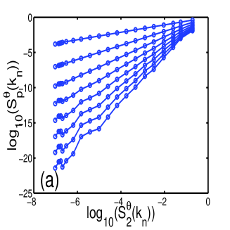
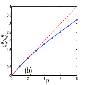
Figure 1: (a) Log-log plots of the order-$p$ structure functions $S_{p}^{\theta}(k_{n})$ versus the second-order structure function $S_{2}^{\theta}(k_{n})$ from our numerical simulations of Model B for $p=1$ (uppermost curve) to $p=8$ (lowermost curve). (b) Plot of the exponent ratios $\zeta^{\theta}_{p}/\zeta^{\theta}_{2}$, obtained from the slopes of the linear, inertial region in (a), versus $p$. Our data points ($\circ$) are connected by a line to guide the eye; the error bars are smaller than the sizes of our symbols; the dashed straight line corresponds to the analogue of the K41 scaling prediction for this case.

We begin the discussion of our numerical results for time-dependent, passive-scalar structure functions in decaying turbulence by comparing our analytical result (37) with data from our simulations of Model B. In Fig. (2a) we show the agreement between the two. The error bars have been calculated as in the the case of equal-time multiscaling exponents: The data we present are the means of the values obtained from 50 different statistically independent runs; and the standard deviations of these values yield the error bars. Here and henceforth time is scaled by the large-eddy-turnover time $t_{L}$. Given the exponential decays of time-dependent passive-scalar structure functions in Models A and B [equations (32) and (37)], we can extract a unique time scale from plots like the one in Fig. (2b). Thus we do not expect time-dependent structure functions to exhibit dynamic multiscaling in Models A and B. In particular, equation (37) implies $T^{\theta}_{2}(k_{n})=[1/4k_{n}^{2-\xi}A(\xi)]^{-1}$ whence $z_{2}=2-\xi.$ For our choice of $\xi=0.6$ we should, therefore, obtain $z_{2}=1.4$, and indeed our numerical simulations yield $z_{2}=1.398\pm 0.003$ [Fig. (2b)]. To demonstrate numerically that higher-order time-dependent structure functions also have a dynamic scaling exponent equal to $z_{2}$, as shown in $Section~{}\ref{analyticB}$ for the fourth-order time-dependent structure function, we show in Figs. (3a) and (3b) our numerical results for the third- and fourth-order time-dependent structure functions versus $t/t_{L}$ for $6\leq n\leq 13$ from which we extract $T^{\theta}_{3}(k_{n})$ and $T^{\theta}_{4}(k_{n})$, respectively. The insets show log-log plots of these times versus $k_{n}$; the slopes of these plots yield the dynamic-scaling exponents $z_{3}=1.398\pm 0.003$ and $z_{4}=1.402\pm 0.005$ in agreement with our expectation $z_{p}=2-\xi$, for all $p$, since $\xi=0.6$ in our calculations.

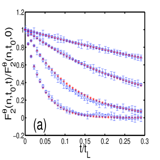
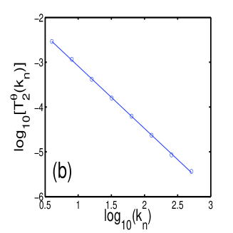
Figure 2: (a) Plots comparing the normalised, second-order, time-dependent structure function versus the dimensionless time $t/t_{L}$ from our numerical simulations (o) of Model B with our analytical expression (37) (*). For clarity we show data for four shells, from $n=6$ (uppermost) to $n=9$ (lowermost). The error bars on our numerical simulations are shown as vertical lines on the data points.
(b) A log-log plot of $T^{\theta}_{2}(k_{n})$ versus $k_{n}$. The slope of this plot gives the dynamic scaling exponent $z_{2}=1.398\pm 0.003$. Our result from numerical simulations agree well with the analytical result $z_{2}=2-\xi$, since we have chosen $\xi=0.6$.

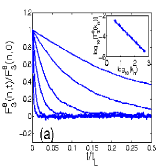
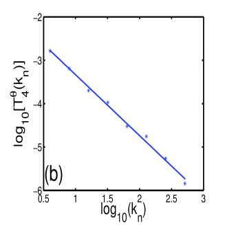
Figure 3: (a) Representative plots of the normalised, third-order time-dependent structure function versus the dimensionless time $t/t_{L}$ from our numerical simulations of Model B for shell numbers $n=6$ (uppermost) to $n=11$ (lowermost). The inset shows a log-log plot of $T^{\theta}_{3}(k_{n})$ versus $k_{n}$. The slope of this plot gives the dynamic scaling exponent $z_{3}=1.398\pm 0.003$, which agrees with $z_{2}$ from Fig. 2b.
(b) A log-log plot of $T^{\theta}_{4}(k_{n})$ versus $k_{n}$. The slope of this plot gives the time-dependent scaling exponent $z_{4}=1.402\pm 0.005$. Our result from numerical simulations agree well with the analytical result $z_{2}=z_{4}=2-\xi$, since we have chosen $\xi=0.6$.

5.2 Model C

The equality of equal-time exponents for decaying and statistically steady fluid turbulence was demonstrated numerically for the Sabra shell model in Ref. [24]. We have carried out a similar exercise for the GOY shell model of fluid turbulence and found, unsurprisingly, that the universality of equal-time multiscaling exponents holds for the GOY model as well. Furthermore, we have also checked that a replacement of the viscous term $\nu_{0}k_{n}^{2}$ in equation (17) by the hyperviscous term $\nu_{\alpha}k_{n}^{2}(k_{n}/k_{d})^{\alpha}$ does not affect these exponents [40].

We investigate now whether time-dependent velocity structure functions in decaying fluid turbulence show a factorisation similar to (32) and (37) for Models A and B. Let us normalise the order-$p$, time-dependent structure function by its value at $t=0$:

$$Q_{p}^{u}(n,t)\equiv\frac{F^{u}_{p}(k_{n},t_{0},t)}{F^{u}_{p}(k_{n},t_{0},0)};$$ (66)

to examine the dependence of $Q_{p}^{u}(n,t)$ on $t_{0}$. We give, in Figure (4a), representative plots of $Q^{u}_{2}(n=9,t)$ and $Q^{u}_{4}(n=5,t)$ versus $t/t_{L}$ for 6 different time origins $t_{0}$; succesive values of $t_{0}$ are separated from each other by $0.5t_{L}$. To the extent that the symbols for different values of $t_{0}$ overlap, our results show that $Q_{p}^{u}(n,t)$ is independent of $t_{0}$ (so we have not included $t_{0}$ as an argument of $Q_{p}^{u}$), i.e., $F^{u}_{p}(k_{n},t_{0},t)$ factorises into a part that depends on $t_{0}$ and another that does not [cf., (32) and (37) for the simple, linear Models A and B]. Clearly the dynamic-multiscaling exponents extracted from $Q_{p}^{u}(n,t)$ cannot depend on $t_{0}$.

Furthermore, these exponents are the same as their counterparts for statistically steady, forced turbulence. We illustrate this in Fig. (4b) by comparing our numerical results for the normalised, time-dependent structure function $F^{f}_{4}(k_{n},t)/S^{u}_{4}(k_{n})$, for statistically steady, forced (superscript $f$) turbulence, and $Q^{u}_{4}(n,t)$. [To obtain a statistical steady state for the GOY shell model we use the external force $f_{n}=(1+\imath)\times 5\times 10^{-3}\delta_{n,1}$.] We have checked explicitly, for $1\leq p\leq 6$, that $Q^{u}_{p}(n,t)$ and $F_{p}^{f}(k_{n},t)/S^{u}_{p}(k_{n})$ agree within our error bars. Hence we propose the following factorisation that relates the time-dependent structure functions for decaying and statistically steady (superscript $f$) turbulence,

$$F_{p}^{u}(k_{n},t_{0},t)=A_{p}(k_{n},t_{0})F_{p}^{f}(k_{n},t),$$ (67)

with all the $t_{0}$ dependence on the right-hand side in the coefficient function $A_{p}$. If we now use the multifractal form for $F_{p}^{f}$ suggested in [6], we obtain the shell-model analogue of equation (64).

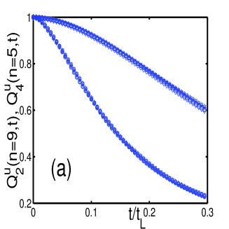
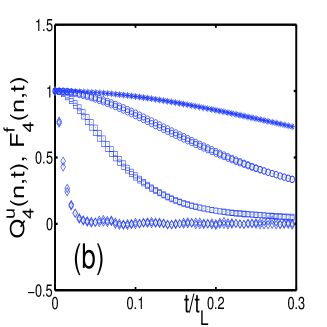
Figure 4: (a) Representative plots of $Q^{u}_{p}(n,t)$ versus the dimensionless time $t/t_{L}$, for $p$=2, $n$=9 (lower curve) and $p=4$, $n$=5 (upper curve), and 6 different time-origins $t_{0}$ in decaying fluid turbulence for Model C. Successive time origins are separated by 0.5$t_{L}$. The different symbols for the different sets of data for the different time-origins are indistinguishable; this is compelling numerical evidence for our proposed factorised form of the time-dependent structure functions.
(b) Plots of $Q^{u}_{4}(k_{n},t)$ and $F^{f}_{4}(k_{n},t)$ as a function of $t/t_{L}$ to numerically test our proposed Ansatz (67) decaying turbulence in Model C. Results are shown only for shells $n=4$ (uppermost curve), 6, 8, and 12 (lowermost curve) for clarity.

We calculate the integral- and the derivative-time scales and their associated exponents $z^{I,u}_{p,1}$ and $z^{D,u}_{p,2}$. The counterparts of equations (49), for $M=1$, and (50), for $M=2$, for the GOY model are :

$$T^{I,u}_{p,1}(n) = \int_{0}^{t_{\mu}}Q^{u}_{p}(n,t)dt;$$ (68)

$$T^{D,u}_{p,2}(n) = \left[\frac{d^{2}Q^{u}_{p}(n,t)}{dt^{2}}\bigg{|}_{t=0}\right]^{-1/2};$$ (69)

here $t_{\mu}$ is the time at which $Q^{u}_{p}(n,t)=\mu$, with $0\leq\mu\leq 1$. In principle we should use $\mu=0$, i.e., $t_{\mu}=\infty$, but this is not possible in any numerical calculation since $Q^{u}_{p}$ cannot be obtained accurately for large $t$. We use $\mu=0.6$; and we have checked in representative cases that our results do not change for $0.3<\mu<0.7$. To compute $T^{D,u}_{p,2}(n)$ we use a centred, finite-difference, sixth-order scheme. Slopes of log-log plots of $T^{I,u}_{p,1}(n)$ and $T^{D,u}_{p,2}(n)$ versus $k_{n}$ $(4\leq n\leq 14)$ give us $z^{I,u}_{p,1}$ (Fig 5a) and $z^{D,u}_{p,2}$ (Fig 5b), respectively.

Our results for equal-time and dynamic-multiscaling exponents for the GOY model (for both types of initial conditions) are given in Tables 1 and 2, respectively. We compute the multiscaling exponents for equal-time and time-dependent structure functions for 50 different cases. Tables 1 and 2 list the means of these values and their standard deviations yield the error bars. By comparing columns 2 of Tables 1 and 2 with column 2 of Table II in Ref. [6] we confirm, for the GOY model, the weak version of universality [24], i.e., the equal-time exponents $\zeta^{u}_{p}$ are the same for both decaying and statistically steady turbulence. Furthermore, our exponents for the GOY shell model agree with those presented in Ref. [24] for the Sabra shell model.

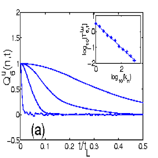
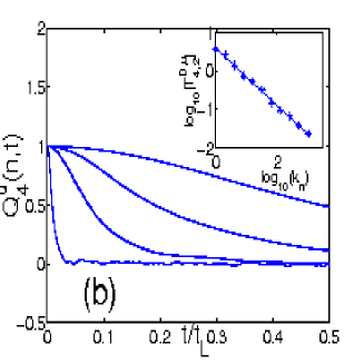
Figure 5: (a) Representative plots of $Q^{u}_{6}(n,t)$ versus $t/t_{L}$ for Model C; for clarity we show shell numbers $n$ = 4 (uppermost), 6, 8 and 12 (lowermost). The inset shows $T^{I,u}_{6,1}(n)$ versus $k_{n}$ on a log-log scale. A linear fit yields the dynamic-multiscaling exponent $z^{I,u}_{6,1}=0.76\pm 0.02$.
(b) Representative plots of $Q^{u}_{4}(n,t)$ versus $t/t_{L}$ for the same shell numbers as in (a). The inset shows $T^{D,u}_{4,2}(n)$ versus $k_{n}$ on a log-log scale. A linear fit yields $z^{D,u}_{4,2}=0.76\pm 0.01$.

A comparison of the remaining columns of Tables 1 and 2 with their counterparts in Table II of Ref. [6] shows that this weak universality also applies to dynamic multiscaling exponents. Moreover, our direct numerical results for $z^{I,u}_{p,1}$ and $z^{D,u}_{p,2}$ (columns $4$ and $6$ in Tables 1 and 2) agree with the bridge-relation values of these exponents (columns $3$ and $5$ in Tables 1 and 2) that follow from equations (53) and (54) and $\zeta^{u}_{p}$ (columns 2 of Tables 1 and 2). Note that the agreement between corresponding entries in Tables 1 and 2 shows that our results are insensitive to the type of initial conditions we use. Finally, if we compare these Tables with Table II in Ref.  [6], we find that our dynamic-multiscaling exponents for decaying, homogeneous, isotropic turbulence agree with their counterparts for the statistically steady case. Pictorial comparisons of the data in Tables 1 and 2 and the results of Ref. [6] are shown in Figs. (6a) and (6b) for integral-time (columns $4$ in Tables 1 and 2) and derivative-time (columns $6$ in Tables 1 and 2) exponents. Similarly Figs. (7a) and (7b) compare the dynamic-multiscaling exponents from our direct numerical simulations with the values predicted for them by the bridge relations (53) and (54) and the equal-time exponents $\zeta_{p}^{u}$ given in Tables 1 and 2.

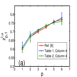
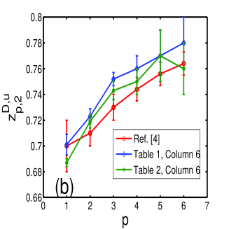
Figure 6: (a) Plots of $z^{I,u}_{p,1}$, with error bars, versus $p$ for Model C with data from  [6], for statistically steady turbulence, and columns 4 of Tables 1 and 2, for decaying turbulence; these plots illustrate the agreement between the three sets of exponents.
(b) We compare the derivative-time exponents $z^{D,u}_{p,2}$ from  [6] and columns 6 of Tables 1 and 2. As in (a), we find that the three sets of exponents agree, within error bars, with each other.

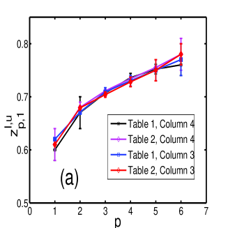
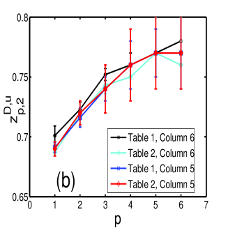
Figure 7: (a) Plots of $z^{I,u}_{p,1}$, with error bars, versus $p$ for Model C with values obtained via the bridge relations (columns 3, Tables 1 and 2) and those obtained from our numerical simulations (columns 4, Tables 1 and 2).
(b)Plots of $z^{D,u}_{p,2}$, with error bars, versus $p$ for Model C with values obtained via the bridge relations (columns 5, Tables 1 and 2) and those obtained from our numerical simulations (columns 6, Tables 1 and 2).

order$(p)$ $\zeta^{u}_{p}$ $z^{I,u}_{p,1}$[Eq.(53)] $z^{I,u}_{p,1}$ $z^{D,u}_{p,2}[Eq.(\ref{zdpm})]$ $z^{D,u}_{p,2}$ 1 0.379 $\pm$ 0.008 0.621 $\pm$ 0.008 0.61 $\pm$ 0.03 0.68 $\pm$ 0.01 0.699 $\pm$ 0.008 2 0.711 $\pm$ 0.002 0.66 $\pm$ 0.01 0.68 $\pm$ 0.01 0.716 $\pm$ 0.008 0.723 $\pm$ 0.006 3 1.007 $\pm$ 0.003 0.704 $\pm$ 0.005 0.711 $\pm$ 0.001 0.74 $\pm$ 0.01 0.752 $\pm$ 0.005 4 1.279 $\pm$ 0.006 0.728 $\pm$ 0.009 0.734 $\pm$ 0.002 0.76 $\pm$ 0.02 0.76 $\pm$ 0.01 5 1.525 $\pm$ 0.009 0.75 $\pm$ 0.02 0.755 $\pm$ 0.002 0.77 $\pm$ 0.02 0.77 $\pm$ 0.02 6 1.74 $\pm$ 0.01 0.78 $\pm$ 0.02 0.78 $\pm$ 0.03 0.77 $\pm$ 0.03 0.78 $\pm$ 0.02

Table 1: Our simulation results for Model C with Type I initial conditions. Order-$p$ (column 1); equal-time exponents $\zeta^{u}_{p}$ (column 2); integral-scale dynamic-multiscaling exponent $z^{I,u}_{p,1}$ (column 3) from the bridge relation (53) and the values of $\zeta^{u}_{p}$ in column 2; $z^{I,u}_{p,1}$ from our calculation using time-dependent structure functions (column 4); the derivative-time exponents $z^{D,u}_{p,2}$ (column 6) from the bridge relation (54) and the values of $\zeta^{u}_{p}$ in column 2; $z^{D,u}_{p,2}$ from our calculation using time-dependent structure function (column 7). The error estimates are obtained as described in the text.

order$(p)$ $\zeta^{u}_{p}$ $z^{I,u}_{p,1}$[Eq.(53)] $z^{I,u}_{p,1}$ $z^{D,u}_{p,2}[Eq.(\ref{zdpm})]$ $z^{D,u}_{p,2}$ 1 0.380 $\pm$ 0.004 0.620 $\pm$ 0.004 0.60 $\pm$ 0.02 0.690 $\pm$ 0.009 0.687 $\pm$ 0.003 2 0.709 $\pm$ 0.003 0.671 $\pm$ 0.007 0.67 $\pm$ 0.03 0.72 $\pm$ 0.01 0.719 $\pm$ 0.005 3 1.000 $\pm$ 0.005 0.709 $\pm$ 0.008 0.707 $\pm$ 0.006 0.74 $\pm$ 0.02 0.743 $\pm$ 0.007 4 1.266 $\pm$ 0.008 0.73 $\pm$ 0.01 0.736 $\pm$ 0.008 0.76 $\pm$ 0.03 0.75 $\pm$ 0.01 5 1.51 $\pm$ 0.01 0.75 $\pm$ 0.02 0.752 $\pm$ 0.009 0.77 $\pm$ 0.03 0.77 $\pm$ 0.02 6 1.74 $\pm$ 0.02 0.77 $\pm$ 0.03 0.76 $\pm$ 0.02 0.77 $\pm$ 0.03 0.76 $\pm$ 0.02

Table 2: Our simulation results for Model C with Type II initial conditions. Order-$p$ (column 1); equal-time exponents $\zeta^{u}_{p}$ (column 2); integral-scale dynamic-multiscaling exponent $z^{I,u}_{p,1}$ (column 3) from the bridge relation (53) and the values of $\zeta^{u}_{p}$ in column 2; $z^{I,u}_{p,1}$ from our calculation using time-dependent structure functions (column 4); the derivative-time exponents $z^{D,u}_{p,2}$ (column 6) from the bridge relation (54) and the values of $\zeta^{u}_{p}$ in column 2; $z^{D,u}_{p,2}$ from our calculation using time-dependent structure function (column 7). The error estimates are obtained as described in the text.

5.3 Model D

From a numerical study of a passive-scalar shell model, with advecting velocities from the Sabra shell model, it was shown [37, 38] that the equal-time scaling exponents $\zeta_{p}^{\theta}$ are universal: they are the same for decaying and statistically steady turbulence; and, in the latter case, they do not depend on the type of forcing. We find, not surprisingly, that this universality holds even when the advecting velocity field is a solution of the GOY model, i.e., for Model D: Table 3 column 2 shows the values of $\zeta_{p}^{\theta}$ for $1\leq p\leq 6$, which we have obtained for decaying turbulence; these agree with the results of Refs. [7, 32] for statistically steady turbulence in Model D. Our equal-time exponents are also within error bars of their counterparts for the passive-scalar shell model of Refs. [37, 38]. We obtain $\zeta_{p}^{\theta}$ from log-log plots such as Fig. (8a) for the modified, equal-time structure function (22) $\Sigma_{p}^{\theta}$ versus $k_{n}$; the slope of the linear region $4\leq n\leq 12$ yields $\zeta_{p}^{\theta}$ that is plotted versus $p$ in Fig. (8b).

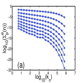
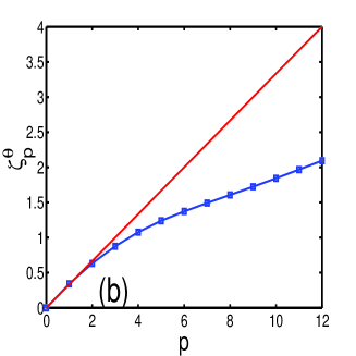
Figure 8: (a) Representative plots of $\Sigma_{p}^{\theta}(n)$ versus $k_{n}$ on a logarithmic scale for $p$ = 1 (uppermost curve) to 8 (lowermost curve) for Model D.
(b) Plot of $\zeta^{\theta}_{p}$, obtained from the linear, inertial region in (a), versus $p$. Our data points, shown as squares, are connected by a line; the error bars are smaller than the size of the symbol. The straight line corresponds to the Kolmogorov prediction of $p/3$.

To analyse the time-dependent, passive-scalar structure functions we follow $Section~{}\ref{c}$ for Model C: We obtain integral- and derivative-time scales from equations (49) and (50), for $M$ = 1 and $M$ = $2$, respectively. In the integral in (49) we set the upper limit to $t_{\mu}$, the time at which the normalised, time-dependent structure function

$$Q_{p}^{\theta}(n,t)\equiv\frac{F^{\theta}_{p}(k_{n},t_{0},t)}{F^{\theta}_{p}(k_{n},t_{0},0)}$$ (70)

is equal to $\mu$, with $0\leq\mu\leq 1$. We use $\mu=0.6$, but we have checked in representative cases that our results remain unchanged if we use the range of values $0.3\leq\mu\leq 0.8$. Slopes of log-log plots of $T^{I,\theta}_{p,1}(n)$ versus $k_{n}$ yield $z^{I,\theta}_{p,1}$. To extract the derivative-time scale, we use a centred, finite-difference, sixth-order scheme to obtain $T^{D,\theta}_{p,2}(n)$ from which we get $z_{p,2}^{D,\theta}$. Integral- and derivative-time multiscaling exponents are extracted from linear fits in the inertial range $4\leq n\leq 10$ as shown in the insets of the representative plots in Figs. (9a) and (9b) for, respectively, $Q_{5}^{\theta}(n,t)$ and $Q_{3}^{\theta}(n,t)$ versus $t/t_{L}$. Finally, from the bridge relations (61) and our GOY-model, equal-time exponents $\zeta_{-1}^{u}=-0.44\pm 0.04$ and $\zeta_{2}^{u}=0.709\pm 0.003$ we obtain $z^{I,\theta}_{p,1}=0.56\pm 0.04$ and $z^{D,\theta}_{p,2}=0.645\pm 0.003$ in agreement with the values from our simulations listed in columns 3 and 4 of Table 3. By comparing these columns with their counterparts in Table II of Ref.  [7], we find agreement, within our error bars, between the dynamic-multiscaling exponents for Model D for both statistically steady and decaying turbulence.

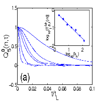
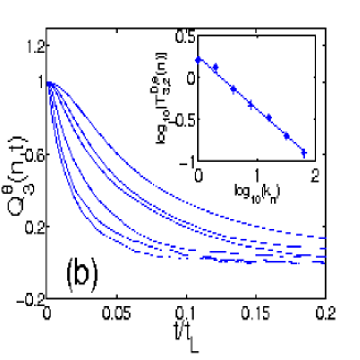
Figure 9: (a) Representative plots of $Q^{\theta}_{5}(n,t)$ versus $t/t_{L}$, for shell numbers 6 (uppermost) to 11 (lowermost) for Model D. The inset shows a log-log plot of $T^{I,\theta}_{5,2}(n)$ versus $k_{n}$. A linear fit yields $z^{I,\theta}_{5,1}=0.562\pm 0.006$.
(b) Representative plots of $Q^{\theta}_{3}(n,t)$ versus $t/t_{L}$ for the same shell numbers as in (a). The inset shows $T^{D,\theta}_{3,2}(n)$ versus $k_{n}$ on a log-log scale. A linear fit yields $z^{D,\theta}_{3,2}=0.646\pm 0.003$.

6 Conclusions

We have systematised the study of the dynamic multiscaling of time-dependent structure functions in four Models (A-D) for passive-scalar (A,B, and D) and fluid (C) turbulence. By a suitable normalisation of these structure functions, we eliminate their dependence on the origin of time $t_{0}$ at which we initiate our measurements. We have shown analytically that for the Kraichnan model of passive-scalar turbulence (Models A and B) the two-point time-dependent structure function can be factorised into two parts, one depending on the origin of time $t_{0}$ and another that does not. This suggests a suitable normalisation of the structure functions by which we can eliminate their dependence on $t_{0}$. Surprisingly the same normalisation works for other models of fluid turbulence (Model C) and passive-scalar turbulence (Model D) as we have shown by extensive numerical simulations. Once this dependence on $t_{0}$ has been factored out, the methods developed earlier [6, 7] for statistically steady turbulence yield linear bridge relations that connect dynamic-multiscaling and equal-time exponents. We show analytically, for Models A and B, and numerically, for Models B, C, and D, that these exponents and bridge relations are the same for statistically steady and decaying turbulence. Thus we have generalised the universality of equal-time exponents [24] and provided strong evidence for dynamic universality, i.e., dynamic-multiscaling exponents do not depend on whether the turbulence decays or is statistically steady for each of the Models A-D. We have shown elsewhere that these exponents do not depend on the dissipation mechanism by studying the GOY model with a hyperviscous term  [40].

It is useful to distinguish our results from other studies of temporal dependences of quantities in turbulence. Two such results are described below.

The first example is the result $E_{tot}(t)\sim t^{-2}$, which holds for the total energy $E_{tot}$ at large times $t$ in decaying turbulence  [1]. This result holds for times that are longer than the time at which the integral length scale becomes comparable to the size of the system. [In decaying turbulence, the integral scale $L_{int}(t)\equiv(\int dkE(k,t)/k)/(\int dkE(k,t))$ increases with time since the large-$k$ part of the energy spectrum $E(k,t)$, at time $t$, gets depleted as $t$ increases.] In all the results we report here, our shell-model analogue of $L_{int}$ is well below the linear size of the system, i.e., $L_{int}\ll k_{0}^{-1}$. Thus our results are not modified significantly by finite-size corrections, nor does the trivial decay of $E_{tot}$, mentioned above, set in and mask the dynamic multiscaling we have elucidated.

The second example is the intermittency of velocity time increments studied in Ref. [41]. These studies calculate structure functions along a single Lagrangian trajectory. Spatial separations, of the sort used in defining equal-time Eulerian structure functions, are replaced by temporal separations along a Lagrangian trajectory. This is distinct from the spatiotemporal structure functions we consider and which are required for a full elucidation of dynamic multiscaling here (and analogous dynamic scaling in critical phenomena).

We have described the way in which we have obtained error bars for the equal-time and dynamic-multiscaling exponents. These error bars only account for statistical errors but not the systematic errors associated with the values of $n$ over which we fit inertial-range exponents. One can try to estimate such systematic errors by obtaining local slopes of log-log plots that yield these exponents. However, local slopes can be deceptive in shell models since the values of $k_{n}$ are separated by factors of 2. Instead, we can try to estimate these systematic errors by comparing the exponents we obtain by fitting over the ranges $3\leq n\leq 15$, $4\leq n\leq 14$, and $5\leq n\leq 13$. We have carried out such checks in representative cases for the dynamic-multiscaling exponents we report. The error bars we then obtain are about a factor of 4 larger than those shown in Tables 1-3.

We hope our work will stimulate experimental studies of dynamic multiscaling in turbulence. Recent advances in the experimental techniques of particle tracking in turbulent flows [42, 43] have made it possible to obtain accurate measurements of Lagrangian properties. To obtain the types of structure functions that we have described it will be necessary at least to track two Lagrangian trajectories of particles that are separated initially by a distance $r$. At the level of second-order structure functions this has been attempted in the direct numerical simulations of Ref. [19].

order$(p)$ $\zeta_{p}^{\theta}$ $z^{I,\theta}_{p,1}$ $z_{p,2}^{D,\theta}$ 1 0.342 $\pm$ 0.002 0.522 $\pm$ 0.002 0.632 $\pm$ 0.003 2 0.634 $\pm$ 0.003 0.531 $\pm$ 0.004 0.647 $\pm$ 0.003 3 0.873 $\pm$ 0.003 0.553 $\pm$ 0.006 0.646 $\pm$ 0.003 4 1.072 $\pm$ 0.004 0.563 $\pm$ 0.003 0.642 $\pm$ 0.005 5 1.245 $\pm$ 0.004 0.562 $\pm$ 0.006 0.643 $\pm$ 0.006 6 1.370 $\pm$ 0.006 0.576 $\pm$ 0.006 0.640 $\pm$ 0.005

Table 3: Our simulation results for Model D. Order-$p$ (column 1); equal-time exponents $\zeta^{\theta}_{p}$ (column 2); integral-scale dynamic-multiscaling exponent $z^{I,\theta}_{p,1}$ (column 3); the derivative-time exponents $z^{D,\theta}_{p,2}$ (column 4). The error estimates are obtained as described in the text.

References

References

- [1] U. Frisch, Turbulence: The Legacy of A.N. Kolmogorov (Cambridge University, Cambridge, England, 1996).
- [2] G. Falkovich, K. Gawedzki and M. Vergassola, Rev. Mod. Phys. 73, 913 (2001).
- [3] V.S. L’vov, E. Podivilov, and I. Procaccia, Phys. Rev. E 55,7030 (1997).
- [4] L. Biferale, G. Bofetta, A. Celani, and F. Toschi, Physica (Amsterdam) 127D, 187 (1999).
- [5] D. Mitra and R. Pandit, Physica (Amsterdam) 318A, 179 (2003).
- [6] D. Mitra and R. Pandit, Phys. Rev. Lett. 93, 2 (2004).
- [7] D. Mitra and R. Pandit, Phys. Rev. Lett. 95, 144501 (2005).
- [8] In our studies of decaying turbulence, we restrict ourselves to initial conditions that lead to a cascade of energy from large to small length scales, where viscous dissipation becomes significant. Certain types of power-law initial conditions[9] do not lead to such a cascade and lead to trivial scaling.
- [9] C. Kalelkar and R. Pandit, Phys. Rev. E, 69, 046304 (2004) and references therein.
- [10] P.C. Hohenberg and B.I. Halperin, Rev. Mod. Phys. 49, 435 (2004) and references therein.
- [11] P.M. Chaikin and T.C. Lubensky, Principles of Condensed Matter Physics (Cambridge University, Cambridge, England, 2004).
- [12] A.N. Kolmogorov, Dokl. Akad. Nauk SSSR 30, 301 (1941).
- [13] A.N. Kolmogorov, Dokl. Akad. Nauk SSSR 31, 538 (1941).
- [14] R. Kraichnan, Phys. Fluids 11, 945 (1968).
- [15] R. Kraichnan, Phys. Rev. Lett. 72, 1016 (1994).
- [16] R. Kraichnan, Phys. Rev. Lett. 78, 4922 (1997).
- [17] A. M. Obukhov, Izv. Akad. SSSR, Serv. Geogr. Geofiz. 13, 58 (1949).
- [18] S. Corrsin, J. Appl. Phys. 22, 469 (1951).
- [19] Y. Kaneda, T. Ishihara, and K. Gotoh, Phys. Fluids 11, 2154 (1999).
- [20] V.I. Belinicher and V.S. L’vov, Sov. Phys. JETP 66, 303(1987).
- [21] D. Mitra, Studies of Static and Dynamic Multiscaling in Turbulence, PhD Thesis, Indian Institute of Science, Bangalore (2005), unpublished.
- [22] E. Gledzer, Sov. Phys. Dokl. 18, 216 (1973).
- [23] K. Ohkitani and M. Yamada, Prog. Theor. Phys. 81, 329 (1989).
- [24] V.S. L’vov, R.A. Pasmanter, A. Pomyalov, and I. Procaccia, Phys. Rev. E 67, 066310 (2003).
- [25] G.I. Taylor, Proc. R. Soc. London, Ser A 151, 421(1935).
- [26] S.B. Pope, Turbulent Flows (Cambridge University, Cambridge, England, 2000).
- [27] A. Wirth and L. Biferale, Phys. Rev. E 54, 4982 (1996).
- [28] P. Perlekar, D. Mitra, and R. Pandit, Phys. Rev. Lett. 97, 264501 (2006).
- [29] S. Dhar, A. Sain, and R. Pandit, Phys. Rev. Lett. 78, 2964 (1997).
- [30] D. Pisarenko, L. Biferale, D. Courvoisier, U. Frisch, and M. Vergassola, Phys. Fluids A 5, 2533 (1993).
- [31] L.P. Kadanoff, D. Lohse, J. Wang, and R. Benzi, Phys. Fluids. 7, 617 (1995).
- [32] M.H. Jensen, G. Paladin, and A. Vulpiani, Phys. Rev. A 45, 7214 (1992).
- [33] J. Zinn-Justin, Quantum Field Theory and Critical Phenomena(Oxford University Press, Oxford, 1999) p.59; this relation is also known as Novikov’s theorem.
- [34] V. S. L’vov and V. L. Lebedev, Phys. Rev. E 47, 1794 (1993).
- [35] F. Hayot and C. Jayaprakash, Phys. Rev. E 57, R4867 (1998).
- [36] F. Hayot and C. Jayaprakash, Int. J. Mod. Phys. B 14, 1781 (2000).
- [37] I. Arad, L. Biferale, A. Celani, I. Procaccia, and M. Vergassola, Phys. Rev. Lett. 87, 164502 (2001).
- [38] Y. Cohen, T. Gilbert, and I. Procaccia Phys. Rev. E 65, 026314 (2002).
- [39] R. H. Kraichnan, V. Yakhot, and S. Chen, Phys. Rev. Lett. 75, 240 (1995).
- [40] R. Pandit, S. S. Ray, and D. Mitra, submitted to European Physical Journal B, arXiv:0709.0893.
- [41] L. Chevillard, S. G. Roux, E. Leveque, N. Mordant, J. -F. Pinton, and A. Arneodo, Phys. Rev. Lett, 95, 064501.
- [42] A. La Porta, G.A. Voth, A.M. Crawford, J. Alexander, and E. Bodenschatz Nature 409, 1017 (2001).
- [43] N. Mordant, J. Delour, E. Leveque, A. Arneodo, and J. -F. Pinton, Phys. Rev. Lett, 89, 254502.