Multifractality in the Random Parameters Model

Abstract

The Random Parameters model was proposed to explain the structure of the covariance matrix in problems where most, but not all, of the eigenvalues of the covariance matrix can be explained by Random Matrix Theory. In this article, we explore other properties of the model, like the scaling of its PDF as one take larger scales. Special attention is given to the multifractal structure of the model time series, which revealed a scaling structure compatible with the known stylized facts for a reasonable choice of the parameter values.

1 Introduction

The problem of determining the correct structure of the correlation matrix is an important one in several different applications. In order to explain that structure of the correlations in different problems, Random Matrix Theory (RMT) [1, 2] has been used in many areas, such as magnetic resonance images [3], meteorology [4], and financial time series [5, 6]. This suggests that much of the structure of the correlation matrix is due to noise.

In Finance applications, the estimation of the correlations is a fundamental for portfolio choice [7]. However, RMT does not claim to explain all the eigenvalue spectrum of financial time series, since a few large eigenvalues remain outside its scope. Also, a number of results have been observed that are not in perfect agreement with RMT, such as the observation that noise eigenvalues seem to be a little larger than expected [8] and that correlations can be measured in the supposedly random part of the eigenvalue spectrum [9, 10]. It has also been verified different behaviors of the eigenvalues corresponding to different points of time, suggesting that non-stationary effects might play an important role [11, 12].

The Random Parameter model, recently proposed by one of the authors [13, 14], tries to fit the complete structure of the correlation matrix, based on parameters that can be interpreted as typical observations of the system. However, more than just explaining the covariance structure, a model for financial time series should also exhibit other empirical properties called stylized facts [15], such as volatility clustering, fat tails and multifractal long range correlations. Here, we will explore the consequences of the Random Parameter model under those aspects. The former two (volatility clustering and fat tails) are studied with usual statistical approaches, whereas the later (multifractal correlations), can be studied using the autocorrelation functions, power spectral densities (either from Fourier or wavelets transforms) and probability distribution functions. In addition, the fractal and the multifractal analysis provide more insights on the scaling exponents. Here we use the singularity spectrum obtained from the Wavelet Transform Modulus Maxima (WTMM) method [17, 18] to determine the multifractal structure of signals generated by this model.

The paper is organized as follows. In Section 2 we describe the model and present some statistical properties related to the PDF’s and the moments for the simulated return time series. Section 3 explains the multifractal concept and the method used to detect it. The results of the multifractal analysis are discussed in the Section 4. Finally, in the last section we present our conclusions.

2 The Model

Here, the returns $\mu_{i}$ and the correlation matrix $P_{il}$, where both $i=1,\cdots,N$ and $l=1,\cdots,N$ refer to the assets, will obtained from a $N\times P$ matrix $\mathbf{\Phi}$, that can be a function of the time $t$, $\mathbf{\Phi}$(t). The matrix $\mathbf{\Phi}$ components $\varphi_{ij}$, where $i=1,\cdots,N$ represents the different assets and where each value of $j$, $j=1,\cdots,P$, $P\geq 3$, can be seen as a collection of $P$ vectors $\mathbf{\varphi}$, each with $N$ components. Each one of those vectors represents a possible, typical state of the system and they are divided in two types of vectors, $M$ main vectors, corresponding to the true parameters of the model, and $R$ secondary ones, randomly drawn at each time as explained bellow, where $M+R=P$.

Given $\mathbf{\Phi}$ and the average return vector $\mathbf{\mu}$, the covariance matrix $\mathbf{\Sigma}$ and the correlation matrix $\mathbf{P}$ will be given by

$$\mu_{i}=E\left[\varphi_{i}\right]=\frac{1}{M}\sum_{j=1}^{M}\varphi_{ij}$$

$$\Sigma_{il}=\frac{1}{M}\sum_{j=1}^{M}\varphi_{ij}\varphi_{lj}-\mu_{i}\mu_{l},$$ (1)

$$P_{il}=\frac{\Sigma_{il}}{\sqrt{\Sigma_{ii}\Sigma_{ll}}}.$$

The observed (simulated) returns $r_{i}(t)$, at instant $t$, are generated, as usual, by a multivariate normal $N(\mu,\Sigma)$ likelihood.

In this model, the $M$ vectors are associated with the permanent, non-random, eigenvalues of the correlation matrix. The $R$ pseudo-parameters will cause the return vector and correlation matrix to change in time, even in the stationary case where each of the $\varphi_{ij}$ elements are held constant (at least, for finite values of $R$) and are the responsible for the bulky region of the correlation matrix eigenvalues. They are drawn according to a Normal distribution $N(0,\Sigma_{ii})$ for each asset $i$.

An interesting aspect of this choice of parameters is that it allows for the introduction of non-stationarity in the main paremeters, while preserving, by definition, all the properties of the correlation matrix. That can be done by making each of the components $\varphi_{ij}$ follow a random walk, such as $\varphi_{ij}(t+1)=\varphi_{ij}(t)+\sigma_{\epsilon}$. However, for long periods of time, this causes the variance associated with each asset to explode and a mean reversal term becomes necessary.

$$\varphi_{ij}(t+1)=(1-\alpha)\varphi_{ij}(t)+\sigma_{\epsilon},$$ (2)

where $\alpha$ is a small number that measures the strength of the mean-reversal process ($\alpha=0$ corresponds to no mean-reversal, while $\alpha=1$ means that the system has no memory of its previous states).

The choice of $\alpha$ and $\sigma_{\epsilon}$ is equivalent to a choice of a value for variance for the $\varphi_{ij}$ that tends to remain the same for the next time instant. This can be seen by calculating the variance of Equation 2 and equating the variances of $\varphi_{ij}$ for $t$ and $t+1$ and one obtains that the variances tend to the point

$$\sigma_{\epsilon}^{2}/(2\alpha-\alpha^{2}).$$ (3)

This point corresponds to the variance value around which the variance of $\varphi_{ij}$ will oscillate.

One important particular case for the purpose of the present analysis is when we make $\alpha=\sigma_{\epsilon}=R=0$. With this choice, the $M$ main vectors will not change in time and, since no random vectors are introduced, this choice means that the average returns and correlation matrix will also not change and we have a simple random walk model for the observed returns, following a Normal distribution, with a correlation matrix with $M-1$ non-zero eigenvalues. This fact can be used to make comparisons with the cases where the returns and correlation matrix do change.

The basic statistical characterization of the actual model was presented in [13, 14]. The next section introduces the wavelet transform modulus maxima method for multifractal analysis.

3 Multifractal analysis

The multifractal scaling analysis have been largely used in the study of turbulence and financial markets [19, 20]. A first access to the multifractal scaling can be done using the Structure Function (SF) analysis. The SF are defined in the following way [16]:

$$S_{q}(Y,\tau)\equiv\langle|Y(t+\tau)-Y(t)|^{q}\rangle\propto\tau^{qh(q)},$$ (4)

where $Y_{i}(t)=\sum_{{t^{\prime}}=0}^{t}r_{i}(t^{\prime})$, $\tau$ is the scale and $\langle~{}\rangle$ denotes the ensemble average. The SF can be regarded as a generalization of the correlation functions (when $q=2$). We will also refer to $\tau$ as the scale of analysis. For a signal that is scale invariant and self-similar, the signal is said fractal when $h(q)$ has the same value for all $q$, otherwise, multifractal [21, 22]. The scaling exponent $h$ is known as the Hölder exponent and, although can be computed using the Structure Function approach [16], this method has the disadvantage of not being able to obtain the the scalings of the negative moments. Another feature of the SF methods is its capability to identify nonstationarity in the data. For stationary time series the exponent of $S_{q}(r_{i},\tau)$ is zero, due to the translational invariance of all statistics.

To obtain the full multifractal spectrum, i.e. positive and negative $q$ moments, we make use of the Wavelet Transform Modulus Maxima (WTMM). The wavelet family used in this paper were the $n^{th}$-derivative of Gaussian (DOG$n$), whose wavelet transform has $n$ vanishing moments and removes polynomial trends of order $n-1$ from the signal. Because the scaling properties of the signal are preserved by the wavelet transform, it is possible to obtain its multifractal spectrum using this method. The number of vanishing moments for the wavelet basis ($n$) is chosen to match the order ($n-1$) of the polynomial trends in the signal.

The wavelet transform of a signal $Y(t)$ is defined as:

$$T_{\psi}(\tau,b_{0})=\frac{1}{\tau}\sum^{N}_{t=1}Y(t)\psi^{*}\Big{(}\frac{t-b_{0}}{\tau}\Big{)},$$ (5)

where $\tau>0$ is the scale being analyzed, $\psi$ is the mother wavelet and $N$ is the number of discretized time steps. In this paper, we used $n=4$ for all analyses.

The statistical scaling properties of the singular measures found in time series are characterized by the singularity spectrum, $D(h)$, of the Hölder exponents, $h$, obtained with the WTMM method [17, 18], by the following equations:

$$h(q)=\lim_{\tau\rightarrow 0}\frac{1}{\ln\tau}\sum_{\{b_{i}(\tau)\}}\hat{T}_{\psi}[q;\tau,b_{i}(\tau)]\ln\left|T_{\psi}[\tau,b_{i}(\tau)]\right|=\lim_{\tau\rightarrow 0}\frac{1}{\ln\tau}Z(q;\tau)$$ (6)

$$D(h)=\lim_{\tau\rightarrow 0}\frac{1}{\ln\tau}\sum_{\{b_{i}(\tau)\}}\hat{T}_{\psi}[q;\tau,b_{i}(\tau)]\ln\big{|}\hat{T}_{\psi}[q;\tau,b_{i}(\tau)]\big{|}=\lim_{\tau\rightarrow 0}\frac{1}{\ln\tau}Z^{*}(q;\tau)$$ (7)

where

$$\hat{T}_{\psi}[q;\tau,b_{i}(\tau)]=\frac{\left|T_{\psi}[\tau,b_{i}(\tau)]\right|^{q}}{\sum_{\{b_{i}(\tau)\}}\left|T_{\psi}[\tau,b_{i}(\tau)]\right|^{q}}$$ (8)

and the summing is over the set of the WT modulus maxima [23] at scale $\tau$, ${\{b_{i}(\tau)\}}$. The singularity spectrum, i.e., the dependence of $D(h)$ with the Hölder exponents, $h$, is obtained from the scaling range on the linear-log plots of Equations (6) and (7). The whole procedure is now a standard [24] and, for brevity, it is not repeated here.

One way to interpret the multifractal spectrum in a physical sense is by comparison with the Hurst exponents expected for known signals, for instance, the fractional Brownian motion [22, 26]. The fractional Brownian motion can be classified following the probabilities of its fluctuations: the usual Brownian motion, obtained from the integration of a Gaussian distributed white noise, has the same probability of having positive or negative fluctuations and has $H=0.5$. A fractional Brownian motion with $H<0.5$ is more likely to have the next fluctuation with opposite sign of the last one – it is said to be antipersistent. Reversely, a fractional Brownian motion with $H>0.5$ is more likely to have the next fluctuation with the same sign of the last one – it is said to be persistent. Antipersistent signals have more local fluctuations and seem to be more irregular in small scales. Their variance diverges slower with time than the variance of persistent signals. The latter ones fluctuate on larger scales and seem to be smoother. This discussion is done in [24] and a similar, but more detailed interpretation is given in [27].

4 Simulations and Results

In order to study the multifractality effects for different values of $\alpha$ and $\sigma_{\epsilon}$, simulations of time series with $2^{15}+2^{14}$ observations each, where the first $2^{14}$ were ignored as transient, were performed. The parameters $\alpha$ and $\sigma_{\epsilon}$ were chosen in a way that they follow the curve that keeps the variance constant, that is $\sigma_{\epsilon}$ was calculated from $\alpha$ by Equation 3. The different values for $\alpha$ were chosen in the interval between $\alpha=0$ (and therefore $\sigma_{\epsilon}=0$, meaning the true parameters remain constant) and $\alpha=1$, when there is no memory and the previous values of the true parameters are forgotten at each time step and new ones are generated. Different numbers of random vectors ($R=1$, 2, 5 and 10) were also chosen for the simulations, in order to investigate the effects of introducing more randomness in the model (as $R\rightarrow\infty$, the model tends to the Random Matrix Theory model for the problem, except for the bulk eigenvalues).

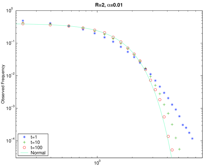
An interesting property of the model is how the observed distributions scale when we take larger time . For a window of one observation, $t=1$, the model clearly shows fat tails. As expected, if we take windows of larger size, the distributions converge to the Normal. Figure 1 shows the observed upper tail of the distribution for the different window sizes and it is typical of what we observe for different values of the parameters, even though the convergence may happen at different rates. The curves correspond to the average over 10 different realizations of the problem. It is easy to see that for larger windows, the curve tends to the Normal distribution.

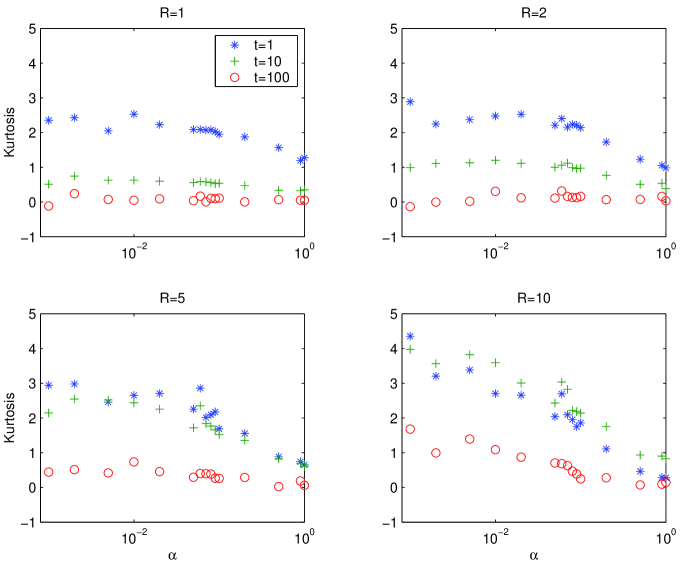
The effect of the choice of the values of $R$ and $\alpha$ on the tails can be better observed in Figure 2, where average values of the kurtosis (averaged over the 10 realizations) are shown. Again, as the window size increases, we get closer to the Normal distribution, with kurtosis of 0. However, other properties can also be observed. Notice that, as $R$ increases, so does the kurtosis for most values of $\alpha$. Near $\alpha=1$, the kurtosis becomes closer to zero for all cases. It is interesting to notice that, as was observed in a previous work [14], when $R$ grows, the eigenvalues of the correlation matrix tend to those of a Random Matrix model, suggesting that large values of $R$ might be associated with a gaussian noise. But Figure 2 shows it clearly that the observed noise has much fatter tails. The obvious conclusion is that, in that region, while the covariance structure tends to the results of Random Matrix, as $R$ grows, the PDFs have much fatter tails than a gaussian PDF.

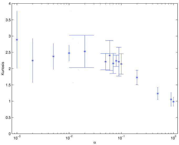
The error bars associated with the different realizations are not shown in Figure 2 to avoid cluttering. Instead, Figure 3 shows the errors for the averages, when $S=2$, for a time window of one. Notice that the error is large for small values of $\alpha$ (meaning that different realizations provide different values for the kurtosis) and decreases as $\alpha$ goes closer to 1. This behavior is typical and observed in the other cases.

The fact that a larger value of $R$ means that larger time windows are necessary to ensure convergence to a Normal distribution can be explained by the fact that the random parameters are randomly drawn using the covariance matrix of the previous time instant. Since the $R$ random vectors influence this matrix, as $R$ grows larger, the changes in the volatility will take a larger time to happen and this should make the convergence slower, as it was observed. This fact suggests that large values of $R$ are useful for describing higher frequency data, while smaller values of $R$ should fit lower frequency observations better.

Another interesting step in the exploration of the model was to check the stationarity of the returns time series, $r$. One signal is said stationary if it is statistically invariant under translations, what can be evaluated using the SF approach [16]. A stationary signal will have a flat, horizontal, structure function plot, $S_{q}\times\tau$. As it is evident from Eq. 4, a stationary signal presents $h=0$ for all values of $q$ and $\tau$ ranges. This procedure determines the range of stationary scales for $\tau$, inside which we should look for the scaling regimes of the price time series, $Y$. If there is such a scale range, we then check for the linear or non-linear behavior of $q.h(q)\times q$, what reveals, respectively, the fractal or multifractal time series dynamics. For all values of $R$ studied, the model presented multifractal scaling for intermediary values of $\alpha$. Although the SF approach had shown the multifractal character of the model, it is not able to work with negative values of $q$, necessary to obtain the full multifractal spectrum, what was done with the WTMM technique, described previously, in section 3.

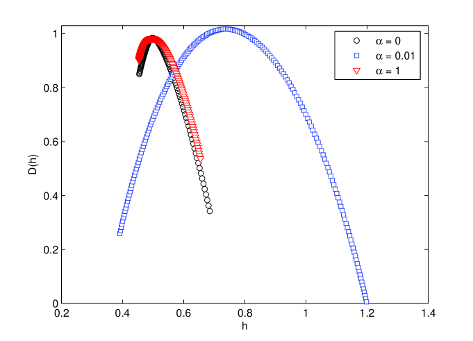
To proceed with the analyses, we used the WWTM method to obtain the multifractal spectrum of $Y$, presented in Fig. 4. This figure shows the multifractal spectrum for $\alpha=0,\>0.01$ and $1$. For both extrema, the MS spectra are much narrower than for the intermediary value $\alpha=1$. Both techniques, SF and WTMM, had been successfully applied in the study of simulated and experimental time series [24, 25] and the intermediary steps to obtain the multifractal spectrum will not be shown in detail here. The interested reader is referred to the cited bibliography.

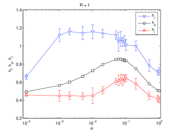
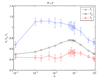
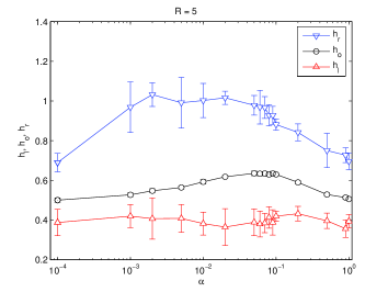
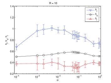
Now we will look for the multifractal properties of the model dynamics as a function of the model parameters $R$ and $\alpha$. The multifractal spectrum may be represented by its extrema points, i.e., its minima on the left, $h_{l}$, and on the right, $h_{r}$, as well as the maximum (top), $h_{0}$. It worths to note that wider the spectrum, i.e. bigger the difference between $h_{r}$ and $h_{l}$, more evident it is the multifractality character. Fig. 5 shows that the multifractal spectrum is narrow for small and high values of $\alpha$. The smallest value simulated was $\alpha=0$, a system with no mean-reversal. The highest, $\alpha=1$, is also non-realistic, since it represents a system with no memory. As it was already expected, these regions are clearly fractal, since the time series for the returns are probably close to gaussians (zero kurtosis). For intermediary values, $\alpha\sim 0.01$, values close to what would be spected in real markets, the multifractal spectrum is wide, a sign of multifractality. In this and all other figures we used time series of 32k points long – for longer time series, the multifractal spectrum for small and high $\alpha\,$’s almost collapses into a single point, indicating a tendency to fractal behavior.

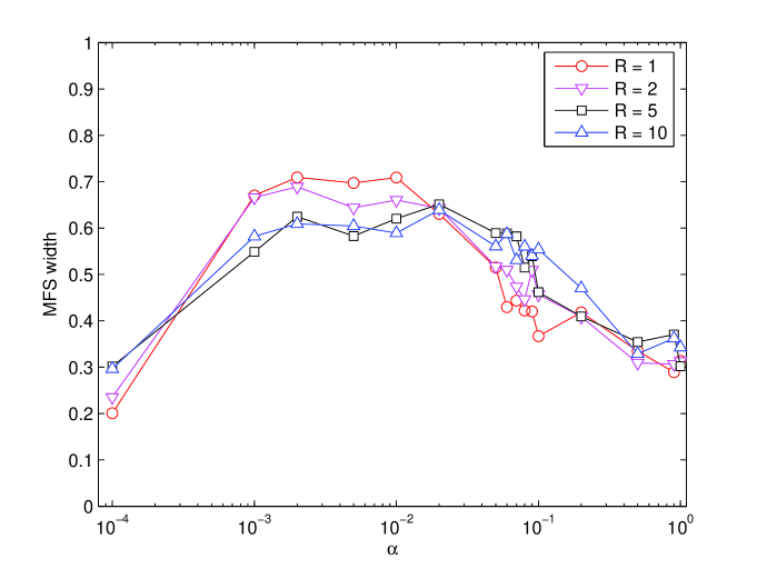
The multifractal character of the time series is more evident from the plot for the spectrum width as a function of $\alpha$, shown in Fig. 6. This figure shows the difference between the maximum and the minimum values of $h$ for each value of $\alpha$, for all four values of $R$ studied ($R=1,\;2,\;5$ and $10$). As $\alpha$ increases, the spectrum width goes from a fractal to a multifractal regime and then returns to a fractal one. This transition is smooth exhibiting large fluctuations for $h_{l}$ and $h_{r}$ in the intermediary values of $\alpha$. It worths to note that the point $h_{l}$ shows the scaling of the large fluctuations on the time series, while the $h_{r}$ captures the scaling of the small fluctuations.

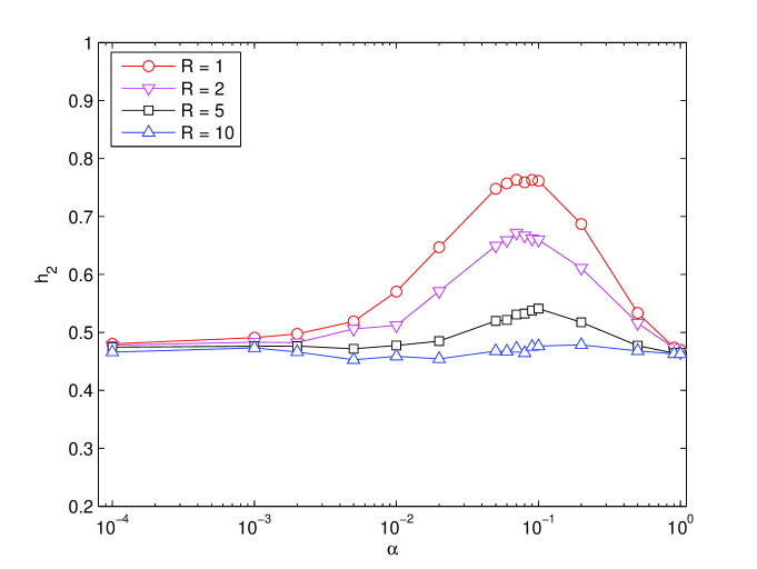
Another representative point of the multifractal spectrum is the value of the Hurst exponent, obtained from $h(q=2)$. As shown by the Fig. 7, the Hurst exponent for small and high values of $\alpha$ is close to $0.5$, the value expected for Brownian random walks. For intermediate, more realistic values $\alpha\sim 0.01$, the time series becomes more persistent, as the Hurst exponent increases, coherent with the real persistent behavior of the market. We could still speculate about the interpretation of the meaning of the $\alpha$ parameter. At intermediary values of $\alpha$, the parameters of the system have some mean-reversal, some memory and the series show increasing values of $H$, all features presented in the real markets. Under this regime, a fluctuation that made the value of the parameters temporarily larger will take longer to bring them back and, therefore, some the observation of persistent behavior makes sense. Under these circumstances, it makes more sense, to predict near future behavior, to use smaller recent series. This is not the case in the no memory and complete memory regimes.

5 Conclusion

The Random Paremeter model was build to explain the covariance structure of time series where non-stationarity might be an important feature, since it allows to implement non-stationarity in the parameters, while trivially respecting the properties of the covariance matrix. We have seen here that the model can also be used to explain other stylized facts, as the multifractal spectrum of financial series. By exploring the PDFs of the generated time series, we have seen how to adapt the model to describe data of high and low frequency; as $R$ is larger, the series match the behavior of high frequency series better. The multifractal spectrum appears when the mean-reversal term is not too large, something that is compatible with real markets. This means that this model is a good choice in describing several properties of the real series and, therefore, should be further investigated.

Figure 1: The tails of the observed probability distributions, averaged over 10 realizations, for different time windows ($t=1$, $t=10$ and $t=100$) for the case $R=2$ and $\alpha=0.01$.

Figure 2: Kurtosis as a function of $\alpha$ for different values of $R$, averaged over 10 realizations. Curves for time windows of size $t=1$, $t=10$ and $t=100$ are shown.

Figure 3: Kurtosis as a function of $\alpha$ for different values of $S=2$, averaged over 10 realizations, with error bars corresponding to the standard deviation of the observed kurtosis over the realizations.

Figure 4: Multifractal spectrum for the model ($R=1$) with $\alpha=0$, $\alpha=0.01$ and $\alpha=1$. It worths to note that the multifractal spectrum for $\alpha=0$ is the same of a fractal Brownian motion with $H=0.5$. All the analyzed signals had 32k points long.

Figure 5: Multifractal spectrum dependence with $\alpha$ for (a) $R=1$, (b) $R=2$, (c) $R=5$ and (d) $R=10$. The error bars are obtained from $10$ realizations.

Figure 6: Multifractal spectrum width as a function of $\alpha$ for all four values of $R$ studied. Surprisingly, all the four values of $R$ have the same width dependence with $\alpha$, although their multifractal spectrum have different absolute values and different values for $h(q=2)$, the Hurst exponent.

Figure 7: The Hurst exponent dependence with $\alpha$ for all the values of $R$ simulated. Curves for increasing values of $R$ show smaller values of the Hurst exponent.

References

- [1] E. P. Wigner, Ann. Math. 53 (1951) 36.
- [2] M. L. Mehta (1967) Random Matrices and the Statistical Theory of Energy Levels. New York, Academic Press, Inc.
- [3] A.M. Sengupta and P.P. Mitra (1999) Distributions of singular values for some random matrices. Phys. Rev. E, 60, 3389-3392.
- [4] M.S. Santhanam and P.K. Patra (2001) Statistics of Atmospheric Correlations, Phys. Rev. E, 64, 016102.
- [5] L. Laloux, P. Cizeau, J.-P. Bouchaud and M. Potters, Phys. Rev. Lett., 83, 1467-1470 (1999)
- [6] V. Plerou, P. Gopikrishnan, B. Rosenow, L. A. N. Amaral, H. E. Stanley, Phys. Rev. Lett., 83, 1471-1474 (1999)
- [7] H. Markowitz, Portfolio Selection, Wiley, New York, 1959.
- [8] J. Kwapień, S. Drożdż, P. Oświeȩcimka, Physica A 359 (2006) 589-606.
- [9] Z. Burda, A. Görlich, A. Jarosz, & J. Jurkiewicz, Physica A (2004) 343, 295-310.
- [10] Z. Burda, & J. Jurkiewicz, Physica A (2004) 344, 67-72.
- [11] S. Drożdż, F. Grummer, A.Z. Gorski, F. Ruf, J. Speth, Physica A 287 (2000) 440.
- [12] S. Drożdż, F. Grummer, F. Ruf, J. Speth, Physica A 294 (2001) 226.
- [13] Martins, André C. R. (2007). Random, but not so much: A parameterization for the returns and correlation matrix of financial time series. Physica A, 383, p. 527-532. doi:10.1016/j.physa.2007.02.108.
- [14] Martins, André C. R. (2007). Non-Stationary Correlation Matrices and Noise. Physica A, 379, 2, p. 552-558. doi:10.1016/j.physa.2006.12.020.
- [15] Rama Count, Empirical properties of asset returns: stylized facts and statistical issues, Quantitative Finance 1 223–236, 2001.
- [16] C.X.Yu, M.Gilmore, W.A.Peebles and T.L.Rhodes, Structure fuction analysis of long-range correlations in plasma turbulence, Physics of Plasmas 10 (7) 2772–2779, 2003.
- [17] J.Muzy, E.Bacry and A.Arneodo, Wavelets and Multifractal Formalism for Singular Signals: Application to Turbulent, Phys. Rev. Lett. 67(25) 3515–3518, 1991.
- [18] A.Arneodo, E.Bacry and J.Muzy, Physica A 213 232–275, 1995.
- [19] U.Frisch Turbulence, Cambridge: Cambridge University Press, 1995.
- [20] F.Schmitt, D.Schertzer and S.Lovejoy, Multifractal fluctuations in finance, Int. J. Theor. App. Fin. 3 361–364, 2000.
- [21] G.Paladin and A.Vulpiani, Phys. Rep. 156(4) 147–225, 1987.
- [22] J.Feder, Fractals, New York: Plenum Press, 1988.
- [23] While we used routines for the wavelet transforms from C. Torrence and G. Compo, available at URL: http://paos.colorado.edu/research/wavelets/, the WTMM method itself was our own implementation.
- [24] K.Bube, C. Rodrigues Neto, R.Donner, U.Schwarz and Ulrike Feudel, Surface characterization of laser beam melt ablation process, Journal of Physics D: Applied Physics 39 1405–1412, 2006.
- [25] E.Faleiro and J.M.G.Gozmez, Multifractal characterisation of fluctuations in simulated Extensive Air Showers, Europhys.Lett. 45 437-443, 1999.
- [26] B.Mandelbrot and J.van Ness SIAM Review 10 422–437, 1968.
- [27] J.B.Cromwell and W.CLabys and E.Kouassi, What color are commodity prices? A fractal analysis, Empirical Economics 25 563–580, 2000.