Statistical Physics of Group Testing
Abstract
This paper provides a short introduction to the group testing problem, and reviews various aspects of its statistical physics formulation. Two main issues are discussed: the optimal design of pools used in a two-stage testing experiment, like the one often used in medical or biological applications, and the inference problem of detecting defective items based on pool diagnosis. The paper is largely based on: M. Mézard and C. Toninelli, arXiv:0706.3104i, and M. Mézard and M. Tarzia Phys. Rev. E 76, 041124 (2007).
1 Introduction
Group testing dates back to 1943, when Dorfman suggested to use it for testing whether US draftees had syphilis [1]. Instead of testing each individual blood sample, the idea is to mix the blood and test pools. In a group of soldiers, one can first test pools of individuals. Then one focuses on the infected pools and performs a second stage of tests on all the individuals belonging to these infected pools. Assuming that each soldier is infected with probability (and that the infections are uncorrelated), the total expected number of tests is
| (1) |
Minimizing this expression over , one finds that the optimal size of the pools is , giving an expected number of tests . If the prevalence of infection is small, , Dorfman’s proposal reduces the total number of blood tests, compared to the individual tests, by a factor .
The general problem of group testing [2] is that of identifying defectives in a set of items by a series of tests on pools of items, where each test only detects whether there exists or not at least a defective item in the pool. It has numerous applications. In particular it is being used in building physical maps of the genome, by detecting whether a special target subsequence of bases is present in a DNA strand [3, 4]. But it has also been suggested to use it in HIV detection [5], in detecting failures in distributed computation [6], or in data gathering in sensor networks [7].
We shall subdivide the group testing problem into two main topics: the pool design (building optimal pools, exploiting the possibility to have overlapping tests), and the inference problem (how to detect defective items, given the results of the pool tests). Two other important classification patterns are the number of stages of detection, and whether one needs to be sure of the result (assuming that the tests are perfect). For instance Dorfman’s design is a two-stage algorithm with sure result. In a first stage one tests the pools, and based on the results of this first stage one designs the second stage of tests, namely the list of all individuals whose blood sample belonged to a defective pool in the first stage. Getting sure results (in contrast to results that hold with high probability) is often needed in medical applications. In order to obtain them, one ends a group testing procedure by a final stage (the second stage in Dorfman’s procedure) which tests individually all the items for which the procedure did not give a sure answer.
In all our study we suppose that the status (’defective’ or ’OK’) of all the items under study are iid random variables: each item can be defective with a probability , or OK with probability . Furthermore we assume that the value of is known. This framework is called ’probabilistic group testing’ in the literature. Another framework has been studied a lot, that of combinatorial group testing where the number of defective items is supposed to be known. Reviews on these two frameworks can be found in [2, 8].
Clearly one can detect defectives more efficiently (with less tests) when more stages can be done. How efficient can one be? Information theory provides an easy lower bound, which applies to the situation where there is no limit on the allowed number of stages. Assume you have a total of items, and you perform tests altogether. There are possible outcomes. If there were defectives, a necessary condition to detect them is that . In the large limit, taking , one finds that the number of tests must be larger than:
| (2) |
It is not difficult to design a sequence of pools, with an unbounded number of stages, which basically reaches this limit.
Clearly, when is small, the minimal number of tests in unbounded number of stage, , is much smaller than Dorfman’s two-stage result . A natural question is that of the minimal number of tests, and the corresponding best pool design, if the number of stages is limited to a value . In the next section we give the answer when , for the case of sure results in two-stage procedures. Amazingly there exist pool designs which require only tests, a factor larger than the optimal unbounded-stage result.
2 Optimal two-stage design in the small limit
In their nice analysis of two-stage group testing, Berger and Levenshtein [9, 10] suggest to study the case where the number of items goes to infinity, and the probability of being defective goes to zero like . In this limit they obtain the following bounds for the minimal expected number of tests required to find all the defectives in two stages, when : .
The recent work of [11] has derived the exact asymptotic minimal expected number of tests, and the pool design which reaches them, when as well as in the limit after . In order to state the results in a compact form, it is convenient to introduce the notation by for the limit where goes to , goes to zero, with and . The limit will be referred to as the case.
The two main results of [11] are the following.
1) If :
| (3) |
2) In these limits, “regular-regular” pools of girth , with tests of degree and variables of degree become optimal with probability tending to one when .
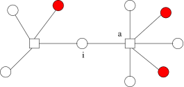
This pooling design is best understood in terms of its factor graph representation. One builds a graph where there are two types of vertices: each variable is a vertex (represented by a circle in figure 1), and each test is also a vertex (represented by a square). An edge is present in the graph, between variable and test , whenever the variable appears in test . The graph is thus bipartite, with edges only between variables and tests. The regular-regular pools correspond to random factor graphs, uniformly drawn from the set of graphs where every variable has degree and every test has degree , and such that the girth (the size of the shortest loop) is at least . The existence of such graph has been demonstrated by Lu and Moura [12]. Their construction is a bit complicated, but a simpler class of graphs has also been shown in [11] to reach optimal performance in the asymptotic limit , with . These are the so-called “Regular-Poisson” graphs where each variable chooses randomly the tests to which it belongs, uniformly among all the possible sets of tests. In such a case the degrees of the tests become asymptotically Poisson distributed, with mean .
The idea of the proof goes in two steps: a general lower bound of combinatorial nature, and a detailed analysis of the previous two random pools designs, showing that their number of tests asymptotically matches the lower bound.
2.1 Lower bound
The lower bound is obtained as follows. Any pool design is characterized by a graph, and therefore by a connectivity matrix with element if item belongs to pool , otherwise. Given a graph and an item with , let us find out the condition for this to be an undetected . This situation occurs whenever any test containing contains at least one item which is defective (see figure 1). If the girth of the graph is larger than , the values of the variables in these neighbouring checks are uncorrelated, and the expected number of undetected in the first stage, for a given graph, is
| (4) |
In general graphs (without any girth condition), one can use a Fortuin-Kasteleyn-Ginibre inequality [13] to show that is always a lower bound to the expected number of undetected in the first stage. Then one minimizes the of eq.(4) over all graphs. This is done using the function which is the fraction of sites such that, among its neighbouring checks, have degree , have degree , etc… Both the total number of checks, and , can be written as linear expressions in . Minimization over is thus easily done.
2.2 Upper bound
It turns out that in the small limit, the undetected s are the dominant sources of errors. One way to see this is through the study of random graph ensembles.
Imagine that the factor graph is generated from an ensemble of graphs where the degrees of the variables and checks are random variables drawn randomly from some fixed distribution. We shall adopt the usual notations from the coding community for describing these degree sequence:
-
•
An item has degree with probability . The sequence of is encoded in the polynomial .
-
•
A test has degree with probability . This is encoded in .
It is also useful to introduce the ’edge perspective degree profiles’. Let be the probability that, when one picks an edge at random in the factor graph, the variable to which it is attached has degree , and be the probability that the test to which it is attached has degree . Then and . These distributions are encoded in the functions and .
Assuming that we have generated a random graph with girth , the various quantities that appear in the computation of the expected number of tests can be expressed in terms of the generating functions.
-
•
The total number of pools in the first stage is: .
-
•
The number of sure OK items (girth ) detected in the first stage is: .
-
•
Number of sure defective items (girth ) detected in the first stage is: .
-
•
All the items which are not detected after the first stage must be tested individually in the second stage. Therefore the total expected number of tests is:
(5) This expression is to be minimized over the degree distributions and .
Some simple probability distributions can be studied efficiently. For instance, the regular regular one, parameterized by and leads to a simple result for in (5). This can be optimized with respect to and for any . figure 2 shows the result.
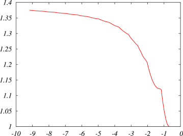
When , it is easy to prove that the optimal values of and are and , and that they saturate the previous lower bound thus providing the exact asymptotic value of the minimal (over all two-stage procedures) number of expected tests: . This is also the case of regular Poisson graphs.
For finite , the best degree sequences are not known. However we have proved that at most coefficients , and at most coefficients are non-zero in these optimal sequences. Plugging this information in some numerical minimization procedure of (5), we have observed numerically that for most values of the optimal degree sequence seems to be the regular-regular one. There are also some values where the optimal graph is slightly more complicated. For instance for , the best sequences we found are and , giving , slightly better than the one obtained with and , giving . But for all values of we have explored, we have always found that either the regular-regular graph is optimal, or the optimal graph has superposition of two neighbouring degrees of the variables, as in this case. In any case regular-regular is always very close to the optimal structure.
3 One stage group testing: inference
Another interesting aspect of group testing, which we now discuss, is the identification of defective items, given a pool design and the results of the tests. This amounts to minimize the number of errors in a one stage experiment. Given a set of pools and the corresponding tests’ results, the identification of the most probable status of each variable is a typical inference problem that can be formalized as follows. Imagine that the items status are given by , where if item is faulty, if it is OK. Then the test returns a signal if , otherwise . Given these test results, one can compute the probability that the items status are given by . This is given by:
| (6) |
Our task is to find the configuration which maximizes this probability. The detection error will be measured by how much differs from .
In order to find , we first use the fact that, whenever a test returns a value , we are sure that all the variables belonging to pool are sure 0: . Therefore we know that . This simple remark leads us to a ’graph stripping’ procedure: We can take away from the graph all tests such that , and all the variables in these pools: they are sure s. The remaining ’reduced graph’ has only tests with . With some slight abuse of notation, let us call the set of variables which remain in this reduced graph (their number is ). The probability distribution on these remaining variables can be written as
| (7) |
The reduced problem can thus be formulated as follows: Find the values of such that:
-
•
For each test in the reduced graph, there is at least one of the variables in its pool that is defective.
-
•
The total number of defective variables should be minimized.
This problem is a version of the celebrated vertex cover problem [14, 15, 16] to the case of a hyper-graph. It is known as the hitting set problem. In the next section we discuss the statistical physics of this problem.
4 Hitting set
The hitting set problem is an interesting problem in itself. In order to get some experience about it, we have studied in [18] the hitting set problem in case of random regular hyper-graphs where tests have degree and variables have degree . We define the weight of a configuration as . The Boltzmann-Gibbs measure of the problem is defined as
| (8) |
We first write the Belief Propagation (BP) equations for this problem. Given a graph and a variable , we consider a sub-graph rooted in obtained by removing the edge between and one of its neighbouring tests, . Define and as the partition functions of this sub-graph restricted to configurations where the variable is respectively OK () or defective (). If the underlying graph is a tree, these two numbers can be computed recursively as follows:
| (9) | |||||
| (10) | |||||
| (11) | |||||
| (12) |
Belief propagation amounts to using these equations on our problem, even if the graph is not a tree. The equations can be simplified by introducing two local cavity fields on each edge of the graph, defined as: , and . They become:
| (13) | |||||
The replica symmetric (RS) solution to this problem amounts to assuming that there is a unique solution to this equation, and in the case of random regular graph it must be a translation invariant solution: and , , with:
| (14) |
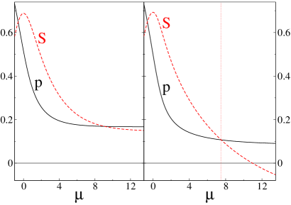
Solving these equations, one can obtain the density of defective items as well as the entropy of the system using the usual formulas for the RS Bethe free energy (see for instance [19]). Figure 3 shows the results for two values of the degree pairs . This shows that the RS solution fails at high chemical potential and low density of active items, at least for and , because it obtains a negative entropy.
A one step replica symmetry breaking (1RSB) solution can be constructed along the lines of reference [19] (see also [20] for an exactly solvable case). They take a particularly simple form in the large limit. In this limit, the survey propagation (SP) equations [21, 22] can be written in terms of one message per edge of the graph. The SP equations for the hitting set problem are [18]:
| (15) |
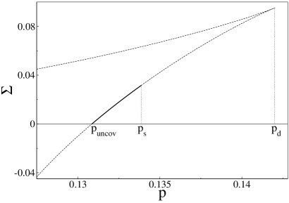
For random regular graphs, the 1RSB solution can be obtained by assuming that is translation invariant, . Equation (15) can be solved easily, and from this solution one can compute, using the technique of [19], the complexity function. In the present case, this function gives times the logarithm of the number of clusters of solutions, versus the optimal density of the cluster . Figure 4 gives the result for the case and . The value of the density where the complexity goes to zero gives the minimal density such that a hitting set exists.
The 1RSB solution is stable to further replica symmetry breaking effects for a wide range of values of the degree pairs . Figure 5 summarizes the nature of the low density phase when one varies and .
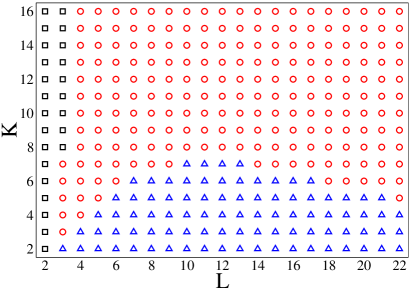
4.1 Survey propagation and survey inspired decimation
As proposed first in [21], the equations obtained from the cavity method can be applied to a single instance of the inference problem, and turned into efficient algorithms. We have studied in [18] two decimation algorithms, one based on the BP equations (13) and one based on the SP equations (15). In both cases the strategy is the same: one iterates the equations in parallel, starting from a random initial condition. If a fixed point is reached, one computes the degree of polarization of each variable. measures to what extent the marginal probability distribution of variable is biased, either towards or towards . In the BP case, is defined as
| (16) |
In the case of SP, it is defined as
| (17) |
The idea of the BP (or SP) inspired decimation algorithm is to identify the most polarized variable from BP (or SP), and fix its value to its most probable value. Then variable is removed from the graph; if the tests connected to are also removed. This procedure is then iterated until all variables are fixed. A subtle issue concerns the values of chosen in BP (resp. the value of chosen in SP). In order to get a better convergence, we compute the entropy versus in the BP case (resp. the complexity versus in the SP case), and fix the value of (resp. ) to the largest value such that the entropy (resp. the complexity) is positive. In this way (resp. ) evolves during the decimation procedure.
In order to get some point of comparison, we have compared the BP and SP inspired decimation to a greedy algorithm, simply defined by the iteration of the procedure: find the variable of largest degree, fix it to , clean the graph. On one instance of a random regular graph with , these three algorithms have obtained some hitting sets with the following minimal densities:
-
•
Greedy algorithm: .
-
•
BP inspired decimation: .
-
•
SP inspired decimation: .
Notice that the prediction from the previous section states that, for , the minimal density necessary to obtain a hitting set, for an infinite graph, should be . On this example, and in various other experiments that we have tried, SP inspired decimation performs slightly better than other algorithms. It would be interesting to extend such comparisons more systematically.
5 Perspectives
Group Testing offers a variety of interesting questions, some of which also have some practical relevance. One of the results that could turn out to be important is the fact that the message passing approaches to the group testing inference problem seem to be fast and efficient. They are also easily generalizable to the case of imperfect tests. One can expect that this will be useful in realistic applications of group testing.
From the point of view of statistical physics, the search for hitting sets gives a new class of problems which exhibits in many cases the general pattern of 1RSB. In these cases, the hyper-vertex cover problem is thus under much better control than the usual vertex cover (which exhibits full RSB). Actually, technically these problems are rather simple to solve even at the 1RSB level. They could thus offer an interesting practice field to develop mathematical tools.
We thank Irina Rish, Greg Sorkin and Lenka Zdeborova for interesting and stimulating discussions. This work has been supported in part by the ’EVERGROW’ EC consortium in the FP6-IST program.
References
- [1] Dorfman D Ann. Math. Statist. 1943 14 436.
- [2] Du D Z and Hwang F K 2000 Combinatorial Group Testing and its Applications (World Scientific: Singapore).
- [3] Barillot E Lacroix B and Cohen D 1991 Nuc. Acids Res. 19 6241.
- [4] Bruno W J Baldings D J Knill E Bruce D Whittaker C Dogget N Stalling R and Torney D C 1995 Genomic 26 21.
- [5] Zenios S A and Wein L M 1998 Stat. Med. 17 1447.
- [6] Zheng A X Rish I and Beygelzimer A 2004 IBM research report RC23441 (W0411-168).
- [7] Hong Y W and Scaglione A 2004 Proc. IEEE Inf. Theory Workshop 298.
- [8] Balding D J Bruno W J Knill E and Torney D C 1996 A comparative survey of nonadaptive pooling designs (T.S Speed and M.Waterman Eds., Springer Verlag: NY).
- [9] Berger T and Levenshtein V I 2002 IEEE Trans. on Inf. Th. 48 1741.
- [10] Berger T and Levenshtein V I 2003 Discrete Applied Mathematics 128 11.
- [11] Mézard M and Toninelli C 2007 Preprint arXiv:0706.3104.
- [12] Lu J and Moura J M F 2006 IEEE Trans. on Magnetics 42 208.
- [13] Fortuin C M Kasteleyn P W and Ginibre J 1971 Comm. Math. Phys. 22 89.
- [14] Frieze A 1990 Discr. Math. 81 171; Gazmuri P 1984 Networks 14 367.
- [15] Weigt M and Hartmann A K 2001 Phys. Rev. E 63 056127; Weigt M and Hartmann A K 2000 Phys. Rev. Lett. 84 6118.
- [16] Weigt M and Zhou H 2006 Phys. Rev. E 74 046110.
- [17] Bauer M and Golinelli O 2001 Eur. Phys. J. B 24 339; Zhou H 2003 Eur. Phys. J. B 32 265; Zhou H 2005 Phys. Rev. Lett. 94 217203.
- [18] Mézard M and Tarzia M (2007 Phys. Rev. E 76 041124.
- [19] Mézard M and Parisi G 2001 Eur. Phys. J. B 20 217; Mézard M and Parisi G 2003 J. Stat. Phys. 111 1.
- [20] Mézard M Ricci-Tersenghi F and Zecchina R 2003 J. Stat. Phys. 111 505.
- [21] Mézard M and Zecchina R 2002 Phys. Rev. E 66 056126.
- [22] Mézard M Parisi G and Zecchina R 2002 Science 297 812.
- [23] Mézard M Tarzia M and Toninelli C in preparation.