Strongly Coupled Plasma Liquids

Abstract

This paper intends to review some of the prominent properties of strongly coupled classical plasmas having in mind the possible link with the quark-gluon plasma created in heavy-ion collisions. Thermodynamic and transport properties of classical liquid-state one-component plasmas are described and features of collective excitations are presented.

1 Introduction

In the RHIC experiments Au+Au collisions at ultra-relativistic energies take place and an extremely high energy density system is created. The experiments demonstrate that a collective state has been created in these nucleus-nucleus collisions, where matter consists of a large number of deconfined quasi-free constituents of the nucleons, namely quarks and gluons. The striking discovery was that these particles are, however, in a strongly interacting phase, resembling a liquid rather than a gas: this phase is being referred to as a strongly coupled Quark Gluon Plasma (sQGP) shuryak07 .

The strongly coupled quark-gluon plasma is in many ways similar to certain kinds of conventional (electromagnetic) plasmas consisting of electrically charged particles (electrons, ions or large charged mesoscopic grains), which also exhibit liquid or even solid-like behavior. These plasmas are known as strongly coupled plasmas and are characterized by an inter-particle potential energy which dominates over the (thermal) kinetic energy of the particles. Strongly coupled plasmas occur in electrical discharges, in cryogenic traps and storage rings, in semiconductors, and in astrophysical systems (interior of giant planets and white dwarfs). Investigations of these physical systems have been a major field of activity for some time Kalmanbook .

Plasmas are extremely versatile, as illustrated in Fig. 1, which shows some plasma types over the density – temperature plane. Besides the more conventional types of plasmas, the approximate location of the sQGP is also shown in Fig. 1.

Figure 1: Different types of plasmas over the density – temperature plane. Note the extremely wide range of these parameters. Strongly coupled plasmas are located right from the $\Gamma$ = 1 line. ($\Gamma$ characterizes the ratio of the potential to kinetic energy, see Eq. (3).)

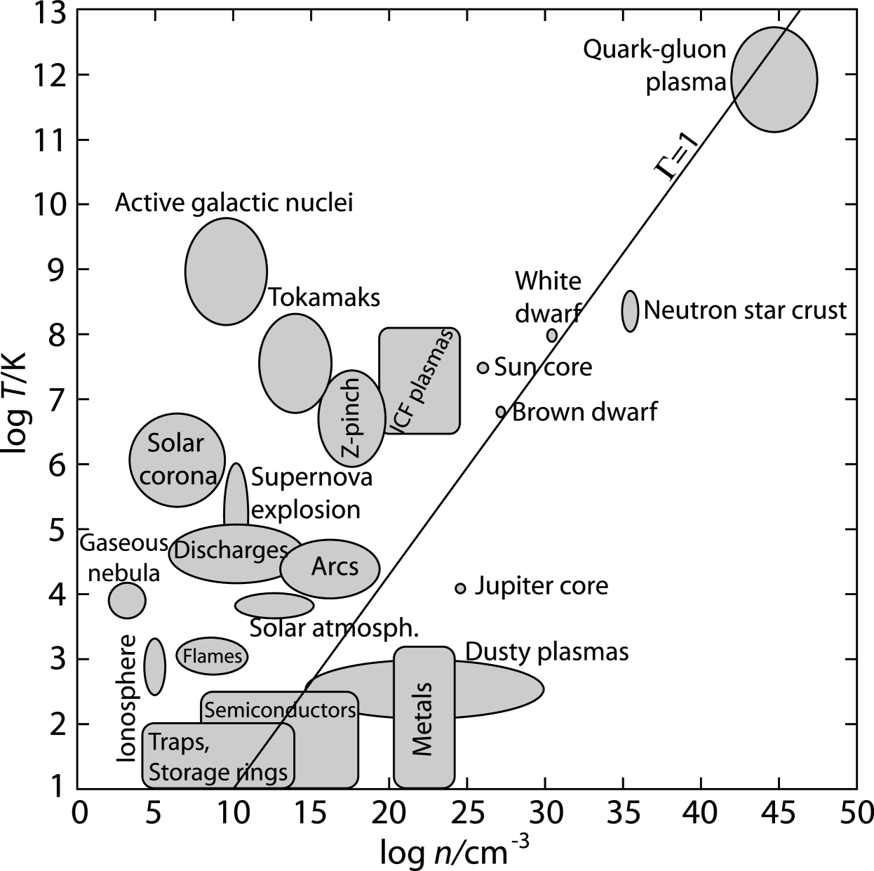
Strongly-coupled plasmas may consist of different charged species. Neutron star crusts are composed of fully stripped iron ions and electrons. Besides electrons, in the core of Jovian planets we find a binary mixture of H⁺ and He²⁺ ions bim , while the core of white dwarf stars consists of a mixture of fully stripped ions of C, N, and O cno . Dusty plasmas, in addition to electrons and ions, also contain another component of mesoscopic dust grains, which charge up and respond to electromagnetic fields similarly as electrons and ions d1 ; d2 ; d3 ; d4 ; d5 .

Part of the different plasmas listed above can be described within the framework of the one-component plasma model (see e.g. BST66 ,) which considers explicitly only a single type of charged species and uses a potential that accounts for the presence and effects of other types of species. This latter may considered as a charge-neutralizing background, which is either non-polarizable or polarizable. In the former case the interaction of the main plasma constituents can be expressed by the

$$\phi(r)=\frac{Q^{2}}{4\pi\varepsilon_{0}}\frac{1}{r}$$ (1)

Coulomb potential energy, whereas in the case of polarizable background the use of the

$$\phi(r)=\frac{Q^{2}}{4\pi\varepsilon_{0}}\frac{\exp(-r/\lambda_{\rm D})}{r}$$ (2)

Yukawa potential energy is appropriate to account for screening effects ($Q$ is the charge of the particles and $\lambda_{\rm D}$ is the Debye length). As examples of systems for which the Yukawa potential can be used, dusty plasmas d1 ; d2 ; d3 ; d4 ; d5 and charged colloids c1a ; c1b ; c2 ; c3 may be mentioned.

Strongly coupled plasmas appear in nature and in laboratory environments in both three-dimensional (3D) and two-dimensional (2D) settings. While 3D systems are more widespread, notable examples of 2D systems are the layer of dust particles levitated in gaseous discharges Thomas94 ; Chu94 and the layer of electrons over liquid helium surface Grimes79 ; tito .

Strongly coupled one-component Coulomb systems are fully characterized by the coupling parameter:

$$\Gamma=\frac{Q^{2}}{4\pi\varepsilon_{0}}\frac{1}{ak_{\rm B}T},$$ (3)

where $a$ is the Wigner-Seitz (WS) radius, and $T$ is the temperature. In the case of Yukawa interaction an additional essential parameter is the screening parameter:

$$\kappa=\frac{a}{\lambda_{\rm D}}.$$ (4)

The coupling parameter $\Gamma$ is the measure of the ratio of the average potential energy to the average kinetic energy per particle. The strong coupling regime corresponds to $\Gamma>$ 1. In the $\kappa\rightarrow 0$ limit the interaction reduces to Coulomb type, while at $\kappa\rightarrow\infty$ it approximates the properties of a hard sphere interaction.

Recent work indicates that the coupling parameter for the sQGP is expected to be in the order of one sQGP (see Fig. 1). This is exactly the reason why methods traditionally used in the mathematical description of strongly coupled plasmas may become useful in the physics of sQGP. Therefore, reviewing the prominent properties of more conventional types of strongly coupled plasmas is of interest and this is indeed the motivation of the present paper. We, on the other hand, do not go beyond the one-component plasma (OCP) model, while a possible description of the sQGP would clearly require a multicomponent plasma model. The methods applicable to single-component systems (such as the ones we deal with in the present paper) serve as the basis of the description of multicomponent systems, such as ionic mixtures bim ; cno ; BIM2 and charged particle bilayers bilayer .

At present, large enough scale numerical simulations, to reproduce e.g. collective excitations, are only feasible for classical systems. Therefore we also restrict our studies (presented here) to classical systems. More sophisticated, but still classical models aiming partial description of sQGP phenomena including electric and magnetic charges were developed by the group of Shuryak shuryak06 . An attempt to include non-Abelian color-color interaction into the classical simulation was presented in QM05 . It is expected that with the advance of computational resources large scale simulations for quantum systems will become realistic within the coming decade.

In Section 2 we introduce the theoretical and numerical methods applied in our studies. Section 3 describes basic thermodynamic properties of the strongly coupled one-component plasma (sOCP). Section 4 deals with the transport properties of sOCP, while Section 5 presents properties of collective excitations characteristic for the liquid phase sOCP. Finally, Section 6 gives a short summary of the paper.

2 Theoretical and numerical methods

Many body systems can be treated theoretically in a straightforward way in the extreme limits of both weak interaction and very strong interaction. In the first case, one is faced with a gaseous system, or a Vlasov plasma, where correlation effects can be treated perturbatively ($\Gamma\ll$ 1). Sophisticated theoretical approaches, like diagrammatic expansions hansensl make it possible to extend standard methods to obtain thermodynamic results in the moderately coupled regime. The random phase approximation (RPA) RPA method, based on the linear response theory, is a useful tool to calculate dynamical properties (wave dispersions) in the case when correlation effects are negligible.

In the case of very strong interaction, the systems crystallize, the particles are completely localized and phonons are the principal excitations. For such conditions lattice-summation techniques serve as solid basis to obtain wave dispersion information.

In the intermediate regime – in the strongly coupled liquid phase – the localization of the particles in the local minima of the potential surface still prevails, however due to the diffusion of the particles themselves the time of localization is finite caging . A successful theoretical approach for calculating structural properties, like the static structure function $S(k)$, is the Hyper-Netted-Chain (HNC) method with the Percus-Yevik (PY) equation HNC .

The localization of the particles (which may typically cover a period of several plasma oscillation cycles) serves as the basis of the Quasi-Localized Charge Approximation (QLCA) method qlca ; qlca2 . The QLCA uses structural information (in the form of static structure function $S(k)$ or the pair correlation function $g(r)$) as input for the calculations of the dispersion relations of the collective modes. The conceptual basis for the QLCA has been a model that implies the following assumptions about the behavior of strongly coupled Coulomb or Yukawa liquids qlca : (i) in the potential landscape deep potential minima form that are capable of trapping (caging) charged particles; (ii) a caged charge oscillates with a frequency that is determined both by the local potential well and the interaction with the other (caged) particles in their instantaneously frozen positions; (iii) the potential landscape changes slowly to allow the charges to execute a fair number of oscillations; (iv) the escape from the cages of the particles is caused by the gradual disintegration of the caging environment; the timescale of this process is determined by the coupling strength $\Gamma$; (v) the (time and velocity dependent) correlation between a selected pair of particles is well approximated by the (time and velocity independent) equilibrium pair correlation; (vi) the frequency spectrum calculated from the averaged (correlated) distribution of particles represents, in a good approximation the average of the distribution of frequencies originating from the actual ensemble. These assumptions have been confirmed to be reasonable in a series of studies (e.g. caging ; qlca2 ).

The main concern of the QLCA theory is the analysis of the collective behavior in strongly coupled many-particle systems. The formal tools for this are the dielectric function $\varepsilon_{\mu\nu}^{AB}({\bf k},\omega)$ [having a tensor character (subscripts) in real space and a matrix character (superscripts) in species space] and the dynamical structure function $S^{AB}({\bf k},\omega)$, or more generally, the dynamical current-current correlation function $T_{\mu\nu}^{AB}({\bf k},\omega)$. The principal approximation of the QLCA method is to replace the fluctuating microscopic densities and their products by their ensemble averages, making use of the $S({\bf k})$ static structure function of the system.

All the information pertaining to the mode structure is contained in the dielectric matrix that has a longitudinal and a transverse element:

$$\varepsilon_{\rm{L/T}}(\textbf{k},\omega)=1-\frac{\omega_{0}^{2}(\textbf{k})}{\omega^{2}-D_{\rm{L/T}}(\textbf{k})}.$$ (5)

Here the $D_{\rm{L}}(\textbf{k})$ and $D_{\rm{T}}(\textbf{k})$ local field functions are the respective projections of the QLCA dynamical matrix $D_{\mu\nu}(\textbf{k})$ qlca , which is a functional of the equilibrium pair correlation function (PCF) $h(r)\equiv g(r)-1$ or its Fourier transform $h(\textbf{k})$:

$$D_{\mu\nu}(\textbf{k})=-\frac{n}{m}\int d^{2}rM_{\mu\nu}(r)[e^{i\bf{k}\cdot\bf{r}}-1]h(r)$$ (6)

with $M_{\mu\nu}(r)=\partial_{\mu}\partial_{\nu}\phi(r)$ being the dipole-dipole interaction potential associated with $\phi(r)$.

The longitudinal and transverse modes are now determined from the dispersion relations

$$\varepsilon_{\rm{L}}(\textbf{k},\omega)=0,\hskip 28.45274pt\varepsilon_{\rm{T}}^{-1}(\textbf{k},\omega)=0.$$ (7)

Besides the theoretical approaches computer simulations have proven to be invaluable tools for investigations of strongly coupled liquids of charged particles. Monte Carlo (MC) and molecular dynamics (MD) methods have widely been applied in studies of the equilibrium and transport properties, as well as of dynamical effects and collective excitations. The main difference between the two techniques is that in a MC simulation independent particle configurations of a canonical ensemble are generated, whereas MD simulations provide information about the time-dependent phase space coordinates of the particles, this way allowing studies of dynamical properties.

Molecular dynamics simulations follow the motion of particles by integrating their equations of motion while accounting for the pairwise interaction of the particles, see e.g. Frenkel . Assuming that the dynamics is Newtonian, for each of the particles the Newtonian equation of motion,

$$m\ddot{\bf r}_{i}={\bf F}_{i}$$ (8)

has to be solved. Here ${\bf F}_{i}$ is the total force acting on the $i$-th particle due to all the other particles and due to any external (e.g. electric and/or magnetic) field. The way how ${\bf F}_{i}$ is calculated will be discussed below. In some physical systems further details have to be considered beyond the Newtonian approximation. As an example charged colloids can be mentioned where the Brownian molecular dynamics simulation c1b ; HL92 is widely used. Brownian molecular dynamics simulations take into account in the equation of motion solvent friction and a random Langevin force ${\bf R}(t)$ acting on the particles.

In the rest of the paper we restrict our studies to systems where Newtonian dynamics is a reasonable approximation. In the case of short-range potentials the calculation of the force acting on a particle of the system, ${\bf F}_{i}$, is relatively simple. In this case MD methods make use of the truncation of the interaction potential thereby limiting the need for the summation of pairwise interaction around a test particle to a region of finite size. In the case of long-range interactions (e.g. Coulomb or low-$\kappa$ Yukawa potentials), which are of interest here, however, such truncation of the potential is not allowed, and thus special techniques, like Ewald summation Ewald , have to be used in MD simulations. Besides the Ewald summation technique there exist few additional methods, like the fast multipole method and the particle-particle particle-mesh method (PPPM, or P3M), which can be used to handle long-range interaction potentials, see e.g. Sagui1999 . It is this latter – widely used Hooker ; David – method, which we also choose as the simulation approach for our studies presented here. The PPPM method was originally applied for the case Coulombic interaction hockney . In the PPPM scheme the interparticle force is partitioned into (i) a force component $F_{\rm PM}$ that can be calculated on a mesh (the “mesh force”) and (ii) a short-range (“correction”) force $F_{\rm PP}$, which is to be applied to closely separated pairs of particles only. In the mesh part of the calculation charged clouds are used instead of point-like particles and their interaction is calculated on a computational mesh, taking also into account periodic images (for more details see hockney ). This way the PPPM method makes it possible to take into account periodic images of the system (in the PM part), without truncating the long range Coulomb or low-$\kappa$ Yukawa potentials. (For high $\kappa$ values the PP part alone provides sufficient accuracy, in these cases the mesh part of the calculation is not used.)

3 One-component plasma properties

Starting with the pioneering work of Brush, Sahlin and Teller BST66 and followed by the systematic studies of Hansen and coworkers Hansen1 ; Hansen2 ; Hansen3 ; Hansen4 properties of one-component plasmas have been explored by computer simulation and theoretical approaches.

In three dimensions (3D) at $\kappa$ = 0 the liquid phase is limited to coupling parameter values $\Gamma\leq 175$ Farouki93 . A first order phase transition was identified to take place at $\Gamma\cong 175$, where the plasma was found to crystallize into bcc lattice SDS90 . We note that at $\kappa>$ 0, the 3D systems may crystallize either in bcc or in fcc lattices, depending on the value of $\kappa$ HFD97 . Crystallization of the plasma was also experimentally confirmed to take place in many different systems, e.g. space plasmas space , in laser-cooled trapped ion plasmas nist and expanding neutral plasmas neutral , as well as in ion storage rings beam1 ; beam2 .

In two dimensions (2D) crystallization into hexagonal lattice occurs at a lower value of coupling, at $\Gamma\approx 137$, as found by both computer simulations Gann79 and by experiments Grimes79 . In two dimensions the crystallized form of the systems is always hexagonal. While most of the studies on 2D system have been carried out in the crystalline state (“plasma crystals”) the liquid state also receives more attention nowadays NG04 ; LG05 .

3.1 Liquid state properties

At high values of the coupling coefficient plasmas exhibit strong structural correlations. Such correlations can easily been studied by examining the pair correlation function

$$g(r)=\frac{V}{4\pi r^{2}N^{2}}\left\langle\lim_{{\rm d}r\rightarrow 0}\frac{1}{{\rm d}r}\sum_{i}\sum_{j\neq i}\int_{r}^{r+{\rm d}r}\delta(\rho-r_{ij})~{}{\rm d}\rho\right\rangle$$ (9)

of the system ($V$ is the volume of the system consisting of $N$ particles). Figure 2(a) shows pair correlation functions for the Coulomb OCP for a series of coupling parameter values, while Fig. 2(b) illustrates the changes of $g(r)$ as a consequence of screening ($\kappa>$ 0). With decreasing $\Gamma$ the peak amplitudes of the pair correlation function decrease, but the positions of the peaks remain nearly unchanged. This remarkable feature of the pair correlation functions indicates that the local environment of the particles in the liquid phase still resembles the underlying ($\Gamma\rightarrow\infty$) lattice configuration. Increasing screening also decreases the degree of correlation as it can be seen in Fig. 2(b).

Figure 2: Pair correlation functions of the classical 3D OCP. Dependence on $\Gamma$ in the Coulomb case (a), and dependence on the screening parameter of the Yukawa potential at fixed coupling $\Gamma$ = 160 (b).

Particle simulation methods provide the full information about the mechanical state of the system (position and velocity of every particle in every discrete time step). However, to extract macroscopic quantities (like thermodynamic energy, pressure, compressibility) it is useful to construct first distribution functions (like the $g(r)$ pair correlation function, being specially important for liquid-state studies, where overall isotropy is a natural assumption) and use the standard tools of classical statistical mechanics (e.g. statphys ) to calculate thermodynamic characteristics.

The total energy of the system can be expressed as:

$$E=\frac{3}{2}Nk_{\rm B}T+U,$$ (10)

which results in

$$\frac{E}{N}=\frac{3}{2}k_{\rm B}T+\frac{n}{2}\int_{0}^{\infty}\varphi(r)g(r)~{}4\pi r^{2}{\rm d}r,$$ (11)

where $U$ is the excess energy, $n$ is the particle number density and $\varphi(r)$ is the interaction pair-potential. The pressure can be calculated using

$$p=nk_{\rm B}T-\frac{n^{2}}{6}\int_{0}^{\infty}\frac{\partial\varphi(r)}{\partial r}g(r)~{}4\pi r^{3}{\rm d}r,$$ (12)

and the isothermal compressibility is expressed by

$$k_{\rm B}T\left(\frac{\partial n}{\partial p}\right)_{T}=1+n\int_{0}^{\infty}\left[g(r)-1\right]~{}4\pi r^{2}{\rm d}r.$$ (13)

The application of the above formulae, derived from fundamental principles of statistical mechanics, depends on the form of the $\varphi(r)$ pair potential. For Coulomb interaction ($\varphi(r)\sim 1/r$) the integral in Eq. (11) is divergent, if the contribution of the uniform neutralizing background is not properly taken into account. This can be done simply by replacing $g(r)$ with $h(r)=g(r)-1$. For Yukawa interaction the contribution of the polarized background is finite ($E_{H}\sim 1/\kappa^{2}$, 3D Hartree energy). The potential energy can be written as the sum of the Hartree energy and the correlational energy:

$$\frac{U_{\rm Yukawa}}{N}=\frac{Q^{2}}{4\pi\varepsilon_{0}~{}a}\left[\frac{1}{\kappa^{2}}+\int_{0}^{\infty}h(\bar{r})\bar{r}e^{-\kappa\bar{r}}{\rm d}\bar{r}\right],$$ (14)

where $\bar{r}=r/a$.

4 Transport properties

In this section we review the data available in the literature for the basic transport coefficients (self-diffusion, shear viscosity and thermal conductivity) of the classical one-component plasma. We mainly present data here for Coulomb OCP, although some data obtained for Yukawa potential at very low values of the screening parameter ($0.01\leq\kappa\leq 0.1$) are also shown for comparison. Transport properties of Yukawa systems characterized by such low $\kappa$ values are very close to those of Coulomb systems. As already mentioned in the introduction, there is a growing interest in Yukawa systems. (For more details about transport properties of Yukawa systems the Reader is referred to the original publications.)

Simulation techniques have become indispensable tools for the determination of transport coefficients. The two main approaches of molecular simulation are the equilibrium and the non-equilibrium methods. In the former one the transport coefficients are derived from correlation functions of microscopic quantities using the Green-Kubo (GK) relations. In non-equilibrium simulations a perturbation is applied to the system and the system’s response is measured.

4.1 Transport coefficients of the classical one-component plasma

4.1.1 Self-diffusion

In equilibrium molecular dynamics simulations one can compute the self-diffusion coefficient $D$ from either the Green-Kubo relation

$$D=\frac{1}{3}\int_{0}^{\infty}\langle{\bf v}(t){\bf v}(0)\rangle{\rm d}t,$$ (15)

(i.e. via the velocity autocorrelation function), or from the Einstein formula:

$$D=\lim_{t\rightarrow\infty}\frac{1}{6t}\langle|{\bf r}_{i}(t)-{\bf r}_{i}(0)|^{2}\rangle,$$ (16)

(i.e. from the mean square displacement of the particles). In the above formulae averaging is taken over particles and different initial times.

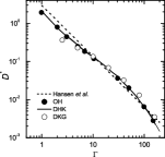
The known for the self-diffusion coefficient are displayed in Fig. 3. The data have been normalized according to $D^{\ast}=D/a^{2}\omega_{0}$, where $\omega_{0}=\sqrt{nQ^{2}/\varepsilon_{0}m}$ is the plasma frequency and $m$ is the mass of theparticles.

Hansen et al. made use of (15) to obtain the self-diffusion coefficient of the Coulomb OCP. Their results were found to follow the approximate relation $D^{\ast}=2.95\Gamma^{-1.34}$ Hansen3 . Ohta and Hamaguchi OHdiff obtained the self-diffusion coefficient for Yukawa liquids from molecular dynamics simulations using (16). Their results for $\kappa$ = 0.1 as well as our present data (based on the same computational procedure) obtained for $\kappa$ = 0 are also shown in Fig. 3. These more recent MD data fall very close to the those given by the above formula.

An additional set of data derived on the basis of the caged behavior and jumping of the particles in the strongly coupled liquid phase caging is also shown in Fig. 3. This data set agrees surprisingly well with the results of the “direct” MD calculations for $D$ over a wide domain of the coupling parameter.

Figure 3: Self-diffusion coefficient of the 3D classical one-component plasma (OCP). Hansen et al: Hansen3 , OH: Ohta and Hamaguchi OHdiff , DKG: Donkó, Kalman and Golden, calculated from cage correlation functions caging , DHK: present MD data. The self-diffusion coefficient has been normalized as: $D^{\ast}=D/a^{2}\omega_{0}$. All data correspond to $\kappa=0$, except OH, which is for $\kappa=0.1$.

4.1.2 Shear viscosity

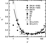
The shear viscosity data for the 3D OCP are shown in Fig. 4. The shear viscosity coefficient has been normalized as: $\eta^{\ast}=\eta/mna^{2}\omega_{0}$.

The shear ($\eta$) and bulk ($\zeta$) viscosity of the 3D OCP was first derived by Vieillefosse and Hansen Hansen4 from the transverse and longitudinal current correlation functions of the plasma. They have found that the shear viscosity exhibits a minimum at $\Gamma\approx$ 20. The other main finding of their work was that the bulk viscosity is orders of magnitude smaller compared to the shear viscosity. The calculations of Wallenborn and Baus WB77 ; WB78 were based on the kinetic theory of the OCP to calculate $\eta$. Their results were in a factor of three agreement with the previous results Hansen4 at $\Gamma$ = 1 and within a factor of two agreement at $\Gamma$ = 160. The minimum value of $\eta$ agreed well for both reports, however the position of the minimum was reported in WB77 to occur at a lower coupling value, $\Gamma\approx$ 8. Molecular dynamics simulation was first applied by Bernu, Vieillefosse and Hansen BVH77 ; BV78 to obtain transport parameters through the Green-Kubo relations. Donkó and Nyíri DN00 used a non-equilibrium MD simulation technique to determine the shear viscosity, while subsequently, Bastea Bastea applied equilibrium simulation and obtained $\eta$ from the Green-Kubo relation. Daligault Jerome has found that the shear viscosity of the OCP follows an Arrhenius type behavior at high $\Gamma$ values. This is shown in Fig. 4 by dashed line.

Salin and Caillol SC have carried out equilibrium molecular dynamics computations for the shear and bulk viscosity coefficients, as well as for the thermal conductivity of the Yukawa one-component plasmas. They have implemented Ewald sums for the potentials, the forces, and for all the currents which enter the Kubo formulas. Saigo and Hamaguchi SH02 have also used the Green-Kubo relations for the calculations of the shear viscosity. As a refinement, the effect of the plasma environment is dusty plasmas has been taken into account through Langevin dynamics in the calculation of shear viscosity of Yukawa systems KAZ .

Figure 4: Shear viscosity coefficient of the 3D classical one-component plasma (OCP). DN: Donkó and Nyíri DN00 using 1024 and 8192 particles, WB: Wallenborn and Baus WB77 ; WB78 , VH: Vieillefosse and Hansen Hansen4 , BV : Bernu et al. BVH77 ; BV78 , B: Bastea Bastea , D: Daligault Jerome , SC : Salin and Caillol SC , SH : Saigo and Hamaguchi SH02 . (The results of Jerome have been scaled to match the minimum value of $\eta$.)

4.1.3 Thermal conductivity

Figure 5: Thermal conductivity coefficient of the 3D classical one-component plasma (OCP). BVH: Bernu et al. BVH77 ; BV78 , DN: Donkó and Nyíri DN00 using 1024 and 8192 particles, SC: Salin and Caillol SC , DH: Donkó and Hartmann DH04 .

Thermal conductivity data for the 3D OCP are shown in Fig. 5. The thermal conductivity coefficient has been normalized as: $\lambda^{\ast}=\lambda/nk_{\rm B}a^{2}\omega_{0}$.

We have reported non-equilibrium molecular dynamics calculation of the thermal conductivity of the classical OCP in DNSH98 . In contrast with the studies of Bernu et al BVH77 ; BV78 where the transport coefficients were obtained from the simulation of an equilibrium system, we applied a perturbation to the system and deduced $\lambda^{\ast}$ from the relaxation time of the system towards the equilibrium state. Donkó and Hartmann DH04 applied the non-equilibrium MD method proposed by Müller-Plathe FMPheat to calculate the thermal conductivity of Yukawa liquids.

As regards to Yukawa systems, transport parameters have been studied in several papers. Besides the work of Salin and Caillol SC (mentioned above), Faussurier and Murillo obtained thermal conductivity (as well as self-diffusion and shear viscosity) values for the Yukawa OCP through its mapping with the Coulomb OCP system, based on the Gibbs-Bogolyubov inequality FM .

5 Collective behavior

Collective excitations (waves) are prominent features of plasmas. Depending on the dimensionality and the confinement of the system, different collective excitations (longitudinal and transverse modes) may show up. Longitudinal modes can fully be characterized by the dynamical structure function $S(k,\omega)$, while transverse modes can be studied through the analysis of the transverse current fluctuation spectra $T(k,\omega)$. The corresponding current fluctuation spectra for the longitudinal mode, $L(k,\omega)$, is linked with the dynamical structure function through $L(k,\omega)=(\omega^{2}/k^{2})S(k,\omega)$. Collective excitations are identified as peaks in these spectra and dispersion relation are derived by observing the change of the frequency (where the peaks are found) with wave number. Additionally, the widths of the peaks in the spectra convey information about the lifetime of excitations (associated with the damping of the waves), as well as about the distribution of the mode frequencies due to the disordered particle configuration in the liquid phase.

Collective effects in Coulomb KG90 ; GKW92 and Yukawa OH2000 ; HO2000 ; RosKal97 plasmas have extensively been investigated. In Coulomb systems the longitudinal (plasmon) mode is known to have a frequency $\omega\rightarrow\omega_{\rm p}$ at $k\rightarrow 0$. The transverse mode exhibits an acoustic dispersion. Rosenberg and Kalman RosKal97 investigated the dispersion relation for dust acoustic waves in a strongly coupled dusty plasma with the aid of the QLCA scheme, generalized to take into account electron and/or ion screening of the dust grains. Hamaguchi and Ohta OH2000 ; HO2000 studied the wave dispersion relations in the fluid phase of Yukawa systems through molecular dynamics simulations. They have demonstrated that the transverse wave dispersion has a cutoff at a long wavelength even in the case of weak screening. Their results have confirmed the earlier theoretical predictions RosKal97 . The QLCA method has subsequently been applied to determine the properties of the transverse (shear) mode in strongly coupled dusty plasmas KRDW00 . For this mode the dispersion was found be characterized by a low-$k$ acoustic behavior and by a frequency maximum lying well below the plasma frequency. The dispersion curves of the longitudinal and transverse modes were demonstrated to merge at high wave number around the Einstein frequency of localized oscillations. Experimental observation of transverse shear waves in the strongly coupled liquid phase of a three-dimensional (layered) dusty plasma have been reported by Pramanik et al. Kaw . The collective modes of dusty plasmas in the liquid phase have also been investigated theoretically by Murillo Murillo1 ; Murillo2 ; Murillo3 .

In the following we present MD simulation results for the collective excitations in 3D Yukawa liquids, and compare these with the predictions of the QLCA theory. The simulations have been carried out using $N$ = 12800 particles. In the MD simulation information about the (thermally excited) collective modes and their dispersion is obtained from the Fourier analysis of the correlation spectra of the density fluctuations

$$\rho(k,t)=k\sum_{j=1}^{N}\exp\bigl{[}ikx_{j}(t)\bigr{]}$$ (17)

yielding the dynamical structure function as Hansen3 :

$$S(k,\omega)=\frac{1}{2\pi N}\lim_{\Delta T\rightarrow\infty}\frac{1}{\Delta T}|\rho(k,\omega)|^{2},$$ (18)

where $\Delta T$ is the length of data recording period and $\rho(k,\omega)={\cal{F}}\bigl{[}\rho(k,t)\bigr{]}$ is the Fourier transform of (17).

Figure 6: Longitudinal current fluctuation spectra in 3D Coulomb OCP at $\Gamma$ = 160 and in a Yukawa OCP at $\Gamma$ = 200, $\kappa$ = 1. $\bar{k}=ka$ denotes the dimensionless wave number, its values are given in (b), while in (a) the arrow indicates increasing values of $\bar{k}$.

Figure 7: Transverse current fluctuation spectra in 3D Coulomb OCP at $\Gamma$ = 160 and in a Yukawa OCP at $\Gamma$ = 200, $\kappa$ = 1. The arrows indicates increasing values of the dimensionless wave number $\bar{k}$ (for values see Fig. 6).

Similarly, the spectra of the longitudinal and transverse current fluctuations, $L(k,\omega)$ and $T(k,\omega)$, respectively, can be obtained from Fourier analysis of the microscopic quantities

$$\lambda(k,t) = k\sum_{j=1}^{N}v_{jx}(t)\exp\bigl{[}ikx_{j}(t)\bigr{]},$$

$$\tau(k,t) = k\sum_{j=1}^{N}v_{jy}(t)\exp\bigl{[}ikx_{j}(t)\bigr{]},$$ (19)

where $x_{j}$ and $v_{j}$ are the position and velocity of the $j$-th particle. Here we assume that ${\bf k}$ is directed along the $x$ axis (the system is isotropic) and accordingly omit the vector notation of the wave number. The way described above for the derivation of the spectra provides information for a series of wave numbers, which are multiples of $k_{\rm min}=2\pi/H$, where $H$ is the edge length of the simulation box. The collective modes are identified as peaks in the fluctuation spectra. The widths of the peaks provide additional information about the lifetimes of the excitations: narrow peaks correspond to longer lifetimes, while broad features are signals for short lived excitations.

Representative longitudinal and transverse current fluctuation spectra, $L(k,\omega)$ and $T(k,\omega)$, respectively, are plotted in Figs. 6 and 7 for wave numbers, which are multiples of $\overline{k}_{\rm min}={k}_{\rm min}a$ = 0.167. $L(k,\omega)$ obtained for the Coulomb case ($\Gamma$ = 160, $\kappa$ = 0) peaks very nearly at the plasma frequency $\omega_{0}$. In the presence of screening (Yukawa potential), as shown in Fig. 6(b), the behavior of $L(k,\omega)$ changes significantly: at $\bar{k}\rightarrow$ 0 the wave frequency $\omega\rightarrow$ 0. The contrast between the $\kappa$ = 0 and the $\kappa>$ 0 cases is also well seen in Fig. 8, where the dispersion curves derived from the fluctuation spectra are displayed. The dispersion curves for $\kappa>0$ are quasi-acoustic ($\omega/\omega_{0}\propto\bar{k}^{1/2}$), with a linear portion near $k$ = 0, which gradually extends when $\kappa$ is increased. The ($\Gamma$,$\kappa$) pairs for which the dispersion graphs are plotted in Fig. 8 have been selected to represent a constant “effective” coupling $\Gamma^{\ast}$ = 160. This definition of $\Gamma^{\ast}$ relies on the constancy of the first peak amplitude of the pair correlation function $g(\bar{r})$, similarly to the case of 2D Yukawa liquids H2005 .

Compared to those characterizing the $\cal{L}$ mode, peaks in the $\cal{T}$ mode spectra are rather broad, as it can be seen in Fig. 7(a) and (b), for the Coulomb and Yukawa cases, respectively. In the case of this mode there is no significant change between the behavior when $\kappa$ changes from zero to a nonzero value, only the mode frequency decreases, as can be observed in Fig. 8(b).

Figure 8: Dispersion relations for the (a) longitudinal and (b) transverse modes of 3D Coulomb and Yukawa plasma liquids. Symbols represent molecular dynamics results, while the lines correspond to the predictions of the QLCA theory. The ($\Gamma,\kappa$) pairs are given in the legend of panel (b).

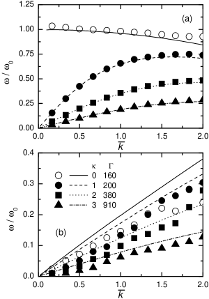
Comparison of the dispersion relations obtained from the MD and QLCA results KRDW00 is presented in Fig. 8. The QLCA equations for the mode frequencies need the pair correlation function as input data. The data shown in Fig. 8 were obtained using MD-generated $g(r)$ functions. The agreement between the (MD and QLCA) dispersion curves is excellent for the $\cal{L}$ mode, while some differences in the frequency of the $\cal{T}$ waves can be seen in Fig. 8(b). This latter may originate from the inaccurate determination of the peak positions of the rather spread $T(k,\omega)$ spectra. Another difference is the cutoff of the $\cal{T}$ mode dispersion curve at finite wave numbers. This disappearance of the shear modes for $k\rightarrow$ 0 is a well known feature of the liquid state Hansen3 ; TK80 ; SZRT97 while the sharp cut-off $\omega\rightarrow$ 0 for a finite $k$ has also been observed in simulations of Yukawa systems OH2000 ; Murillo3 . It is noted that this cutoff is not accounted for by the QLCA, as it does not include damping effects.

6 Summary

This paper intended to review some of the important properties of strongly coupled plasmas (within the framework of the one-component plasma (OCP) model), which might be relevant to the studies of strongly interacting quark-gluon plasma (sQGP).

At high values of the coupling coefficient ($\Gamma\gg 1$) the one-component plasma exhibits liquid state properties. In this domain the pronounced peaks of the pair correlation function indicate the presence of strong correlation effects. The transport coefficients – self-diffusion, shear viscosity and thermal conductivity – have thoroughly been investigated and their behavior is quite well understood. While the self-diffusion coefficient decreases monotonically with increasing $\Gamma$, the shear viscosity and thermal conductivity exhibit a minimum at moderate values of coupling ($10\leq\Gamma\leq 20$), due to the different temperature dependence of the kinetic and potential contributions to these transport coefficients. Two types of collective excitations – a longitudinal and a transverse mode – have been identified in the OCP system, the emergence of latter of them being attributed to strong correlations.

References

- (1) E. Shuryak, [arXiv:hep-ph/0703208v1]
- (2) G. J. Kalman, K. B. Blagoev and M. Rommel, Editors, Strongly coupled Coulomb systems (Plenum Press, 1998).
- (3) J.-P. Hansen, G. Torrie and P. Vieillefosse, Phys. Rev. A 16, 2153 (1977).
- (4) H. Iyetomi, S. Ogata and S. Ichimaru, Phys. Rev. B 40, 309 (1989).
- (5) A. Melzer, V. A. Schweigert, I. V. Schweigert, A. Homann, A. Peters and A. Piel, Phys. Rev. E 54, R46 (1996).
- (6) J. B. Pieper, J. Goree and R. A. Quinn J. Vac. Sci. Technol. A 14, 519 (1996).
- (7) M. Zuzic, A. V. Ivlev, J. Goree et al. Phys. Rev. Lett. 85, 4064 (2000).
- (8) S. Robertson, A. A. S. Gulbis, J. Collwell and M. Horányi, Phys. Plasmas 10, 3874 (2003).
- (9) Z. Sternovsky, M. Lampe and S. Robertson, IEEE Trans. Plasma Sci. 32, 632 (2004).
- (10) S. G. Brush, H. L. Sahlin and E. Teller, J. Chem. Phys. 45, 2102 (1966).
- (11) H. Löwen H, E. Allahyarov, C. N. Likos, R. Blaak, J. Dzubiella, A. Jusufi, N. Hoffmann and H. M. Harreis, J. Phys. A 36, 5827 (2003).
- (12) H. Löwen H, J.-P. Hansen and J.-N. Roux, Phys. Rev. A 44, 1169 (1991).
- (13) A. P. Hynninen and M. Dijkstra, J. Phys. Condens. Matter 15, S3557 (2003).
- (14) S. Auer and D. Frenkel J. Phys. Condens. Matter 14, 7667 (2002).
- (15) H. Thomas, H., G. E. Morfill, V. Demmel, J. Goree, B. Feuerbacher, and D. Möhlmann, Phys. Rev. Lett. 73, 652 (1994).
- (16) J. H. Chu and L. I, Phys. Rev. Lett. 72, 4009 (1994).
- (17) C. C. Grimes and G. Adams, Phys. Rev. Lett. 42, 795 (1979).
- (18) D. C. Glattli, E. Y. Andrei, F. I. B. Williams, Phys. Rev. Lett. 60, 420 (1988).
- (19) M. H. Thoma, J. Phys. G: Nucl. Part. Phys. 31, L7 (2005); M. H. Thoma, J. Phys. G: Nucl. Part. Phys. 31, 539 (2005); T. D. Lee, Nucl. Phys. A 750, 1 (2005); J. Liao and E. Shuryak, Phys. Rev. C 75, 054907 (2007); S. Mrowczynski, M. H. Thoma, Ann. Rev. Nucl. Part. Sci. 57, 1 (2007); J. L. Nagle, Eur. Phys. J. C 49, 275 (2007).
- (20) J. P. Hansen, I. R. McDonald, and P. Vieillefosse, Phys. Rev. A 20, 2590 (1979); S. Ogata, H. Iyetomi, S. Ichimaru, and H. M. Van Horn, Phys. Rev. E 48, 1344 (1993).
- (21) Z. Donkó, G. J. Kalman, P. Hartmann, K. I. Golden, and K. Kutasi, Phys. Rev. Lett. 90, 226804 (2003); S. Ranganathan and R. E. Johnson, Phys. Rev. B 69, 085310 (2004); G. J. Kalman, P. Hartmann, Z. Donkó, and K. I. Golden, Phys. Rev. Lett. 98, 236801 (2007).
- (22) J. Liao and E. Shuryak, Phys. Rev. C 75.
- (23) P. Hartmann, Z. Donko, P. Levai and G. J. Kalman, Nucl. Phys. A 774, 881 (2006).
- (24) J. P. Hansen, I. R. McDonald, Theory of Simple Liquids (Academic Press, London, 1976).
- (25) H. Ehrenreich, M. H. Cohen, Phys. Rev. 115, 786 (1959).
- (26) Z. Donkó, G. J. Kalman and K. I. Golden, Phys. Rev. Lett. 88, 225001 (2002).
- (27) R. Balescu, Equilibrium and Non-equilibrium Statistical Mechanics (Wiley, 1975)
- (28) K. I. Golden and G. J. Kalman, Phys. Plasmas 7, 14 (2000).
- (29) G. J. Kalman, K. I. Golden, Z. Donkó and P. Hartmann, J. Phys. Conf. 11, 254 (2005).
- (30) D. Frenkel and B. Smit, Understanding Molecular Dynamics Simulations (Academic Press, 2001).
- (31) H. Löwen, J. Phys. Condens. Matter 4, 10105 (1992).
- (32) P. P. Ewald, Ann. Phys. 64, 253 (1921).
- (33) C. Sagui and T. A. Darden, Ann. Rev. Biophys. Biomol. Struct. 28, 155 (1999).
- (34) N. David and S. M. Hooker, Phys. Rev. E 68, 056401 (2003).
- (35) N. David, D. J. Spence, and S. M. Hooker, Phys. Rev. E 70, 056411 (2004).
- (36) R. W. Hockhey and J. W. Eastwood, Computer Simulation Using Particles (McGraw-Hill, New York, 1981).
- (37) J. P. Hansen, Phys. Rev. A 8, 3096 (1973).
- (38) E. L. Pollock and J. P. Hansen, Phys. Rev. A 8, 3110 (1973).
- (39) J. P. Hansen, I. R. McDonald, and E. L. Pollock Phys. Rev. A 11, 1025 (1975).
- (40) P. Vieillefosse and J. P. Hansen, Phys. Rev. A 12, 1106 (1975).
- (41) R. T. Farouki and S. Hamaguchi, Phys. Rev. E 47, 4330 (1993).
- (42) G. S. Stringfellow, H. E. DeWitt and W. L. Slattery, Phys. Rev. A 41, 1105 (1990).
- (43) S. Hamaguchi, R. T. Farouki and D. H. E. Dubin, Phys. Rev. E 56, 4671 (1997).
- (44) J. A. Vasut, M. D. Lennek and T. W. Hyde, Adv. Space Research 29, 1295 (2002).
- (45) J. J. Bollinger, T. B. Mitchell, X.-P. Huang, W. M. Itano, J. N. Tan, B. M. Jelenković, and D. J. Wineland, Physics of Plasmas 7, 7 (2000).
- (46) T. Pohl, T. Pattard and J. M. Rost, Phys. Rev. Lett. 92 155003 (2004).
- (47) U. Schramm and D. Habs, Prog. Part. Nucl. Phys. 53, 583 (2004).
- (48) H. Okamoto, Y. Yuri and K. Okabe, Phys. Rev. E 67, 046501 (2003).
- (49) R. C. Gann, S. Chakravarty and G. V. Chester, Monte Phys. Rev. B 20, 326 (1979).
- (50) V. Nosenko and J. Goree, Phys. Rev. Lett. 93, 155004 (2004).
- (51) B. Liu and J. Goree, Phys. Rev. Lett. 94, 185002 (2005).
- (52) D. McQuarrie, Statistical Mechanics (Univ. Sci. Books, 2000).
- (53) H. Ohta and S. Hamaguchi, Phys. Plasmas 7, 4506 (2000).
- (54) J. Wallenborn and M. Baus, Phys. Lett. 61A, 35 (1977).
- (55) J. Wallenborn and M. Baus, Phys. Rev. A 18, 1737 (1978).
- (56) B. Bernu, P. Vieillefosse, and J. P. Hansen, Phys. Lett. 63A, 301 (1977).
- (57) B. Bernu and P. Vieillefosse Phys. Rev. A 18, 2345 (1978).
- (58) Z. Donkó and B. Nyíri, Phys. Plasmas 7, 45 (2000).
- (59) S. Bastea, Phys. Rev. E 71, 056405 (2005).
- (60) J. Daligault, Phys. Rev. Lett. 96, 065003 (2006).
- (61) G. Salin and J.-M. Caillol, Phys. Rev. Lett. 88, 065002 (2002); Phys. Plasmas 10, 1220 (2003).
- (62) T. Saigo and S. Hamaguchi, Phys. Plasmas 9, 1210 (2002).
- (63) K. Dzhumagulova and T. Ramazanov, P07, Abstract Book of the 12th International Workshop on the Physics of Non-Ideal Plasmas, Sept. 4-8, 2006, Darmstadt, Germany
- (64) Z. Donkó, B. Nyíri, L. Szalai and S. Holló, Phys. Rev. Lett. 81, 1622 (1998).
- (65) Z. Donkó and P. Hartmann, Phys. Rev. E 69, 016405 (2004).
- (66) F. Müller-Plathe, J. Chem. Phys. 106, 6082 (1997).
- (67) G. Faussurier and M. S. Murillo, Phys. Rev. E 67, 046404 (2003).
- (68) F. Müller-Plathe, Phys. Rev. E 59, 4894 (1999).
- (69) D. J. Evans and G. P. Morriss, Statistical mechanics of nonequilibrium liquids (Academic Press, 1990)
- (70) G. Pan, J. F. Ely, C. McCabe, and D. J. Isbister, J. Chem. Phys. 122, 094114 (2005).
- (71) G. J. Kalman and K. I. Golden, Phys. Rev. A 41, 5516 (1990).
- (72) K. I. Golden, G. J. Kalman, and P. Wyns, Phys. Rev. A 46, 3454 (1992).
- (73) H. Ohta and S. Hamaguchi, Phys. Rev. Lett. 84, 6026 (2000).
- (74) S. Hamaguchi and H. Ohta, J. Phys. IV France 10, Pr5-19 (2000).
- (75) M. Rosenberg and G. J. Kalman Phys. Rev. E 56, 7166 (1997).
- (76) G. J. Kalman, M. Rosenberg and H. E. DeWitt Phys. Rev. Lett. 84, 6030 (2000).
- (77) J. Pramanik, G. Prasad, A. Sen and P. K. Kaw, Phys. Rev. Lett. 88, 175001 (2002).
- (78) M. S. Murillo, Phys. Plasmas 5, 3116 (1998).
- (79) M. S. Murillo, Phys. Plasmas 7, 33 (2000).
- (80) M. S. Murillo, Phys. Rev. Lett. 85, 2514 (2000).
- (81) P. Hartmann, G. J. Kalman, Z. Donkó and K. Kutasi, Phys. Rev. E 72, 026409 (2005).
- (82) H. Totsuji and N. Kakeya Phys. Rev. A 22, 1220 (1980).
- (83) P. Schmidt, G. Zwicknagel, P.-G. Reinhard and C. Toepffer, Phys. Rev. E 56, 7310 (1997).