Upper Bound of Relative Error of Random Ball Coverage for Calculating Fractal Network Dimension

Abstract

Least box number coverage problem for calculating dimension of fractal networks is a NP-hard problem. Meanwhile, the time complexity of random ball coverage for calculating dimension is very low. In this paper we strictly present the upper bound of relative error for random ball coverage algorithm. We also propose twice-random ball coverage algorithm for calculating network dimension. For many real-world fractal networks, when the network diameter is sufficient large, the relative error upper bound of this method will tend to $0$. In this point of view, given a proper acceptable error range, the dimension calculation is not a NP-hard problem, but P problem instead.

Key Words: Fractal network, Dimension, Random ball coverage

PACS: 89.75.Hc, 89.75.Da, 05.45.Df

1 Introduction

The structure of complex systems across various disciplines can be abstracted and conceptualized as complex networks of nodes and links to which many quantitative methods can be applied so as to extract any characteristics embedded in the system[1, 2, 3]. There exist many types of networks and characterizing their topology is very important for a wide range of static and dynamic properties. Recently, C. Song et al.[4, 5] applied a least box number covering algorithm to demonstrate the existence of self-similarity in many real networks. They also studied and compared several possible least box number covering algorithms, by applying them to a number of model and real-world networks[6]. They found that the least box number covering optimization is equivalent to the well-known vertex coloring algorithm which is a NP-hard problem. It implied that any least box number covering algorithms are heuristic algorithms. Can we avoid the NP-hard problem and simplify the network fractal dimension calculation? In this paper we modify the random sequential box-covering algorithm[7] and presented a random ball coverage algorithm. The relative error smallest upper bound (Supremum) is given theoretically. The simulation experiments shows that no matter how large the network diameter is, this upper bound tends to $0.36$. So we develop another algorithm for calculating dimension which employ only two random ball coverages. We also yield the smallest relative error upper bound of this algorithm, which tend to $0$ when the network diameter is large enough. In this point of view, for a proper acceptable error range, the random ball covering algorithm is equivalent to the least box number covering algorithm in statistic sense when a network is large enough. There is no need to focus on the least box number covering optimization problem when we want to calculate dimension of a large diameter network.

2 Strict upper bounds of random ball coverage

The least box number coverage[6] and random ball coverage were defined as following. For a given network $G$, a box with diameter $r$ is a set of nodes where all distances $d_{ij}$ between any two nodes $i$ and $j$ in the box are smaller than $r$. The least box number coverage is the box coverage with the minimum number of boxes required to cover the entire network $G$. In order to correspond to the fractal network definition[6] we use ’open’ ball to cover the network. So our random ball coverage is little difference with the random sequential box-covering algorithm[7]. A ball with radius $r$ and center node $c$ is the set of nodes which satisfy the shortest path length from the center $c$ to each of them is smaller than $r$. The random ball coverage with radius $r$ as: at each step, we randomly choose a node which has not been covered as a center, and cover all the nodes within the distance $r$ to the center. The process is repeated until all the nodes in the network were covered.

Theorem $1$: $L(2r)\leq$ $B(r)\leq L(r)$, where $L(r)$ is the number of boxes in a lest box number coverage with diameter $r$ and $B(r)$ denotes the number of balls in a random ball coverage with radius $r$.

Proof:

$\because\ \ B(\frac{r}{2})$ can be regarded as the number of boxes in a random box number coverage with diameter $r-1$.

$\therefore\ L(r)\leq L(r-1)\leq B(\frac{r}{2})$

Suppose $L_{1},L_{2},\cdots,L_{m}$ denote all the boxes in a lest box number coverage, where $m=L(r)$, and $L_{1}=\{n_{11},n_{12},\cdots,n_{1k_{1}}\},L_{2}=\{n_{21},n_{22},\cdots,n_{2k_{2}}\},\cdots,\\ L_{m}=\{n_{m1},n_{m2},\cdots,n_{mk_{m}}\}$. Then we have $L_{i}\bigcup L_{j}=\Phi$ for all $i\neq j,i\leq m,j\leq m$, where $\Phi$ denotes empty set.

According to the above definition of random ball coverage with radius $r$, without loosing any generality suppose the center of the first ball in a random ball coverage process is $n_{11}$, then $L_{1}$ is covered by the first ball and the second random ball’s center must lies out of $L_{1}$. Without loosing any generality we also can assume $n_{21}$ is the center of the second ball, then $L_{2}$ is covered by the second ball. In this way, we can get that: $B(r)\leq L(r)$.

$\therefore\ B(r)\leq L(r)\leq B(\frac{r}{2})$

$\therefore\ L(2r)\leq$ $B(r)\leq L(r)$

Theorem $2$: Suppose $G$ is a fractal network, the available box diameter range is $\{m,m+1,\ldots,R\}$ and we employ linear lest squares regression to get the dimension. Then the smallest upper bound of the relative error of dimension calculated by random ball coverage is

$e(R,m)=\frac{\log 2[k\log\frac{R!}{m!}-(R-m+1)\log\frac{(m+k-1)!}{m!}]}{(R-m+1)\sum_{i=m}^{R}{(\log{i})^{2}}-(\log\frac{R!}{m!})^{2}}$

where, $k\in\{1,2,\cdots,R-m+1\}$ and satisfy: $\log(m+k-1)\leq\frac{\log\frac{R!}{m!}}{R-m+1}\leq\,\log(m+k)$ Proof:

$\because$ network $G$ is fractal in range $\{m,m+1,\ldots,R\}$.

$\therefore$ there must exist a proper $b$ for any $r\in\{m,m+1,\ldots,R\}$ such that

$$\log_{a}L(r)=-s\log_{a}r+b$$ (1)

$$\log_{a}L(2r)=-s\log_{a}r+b-s\log_{a}2$$ (2)

Then

$$\log_{a}B(r)=-s\log_{a}r+b-\theta_{r}s\log_{a}2,\theta_{r}\in[0,1]$$ (3)

where, $s$ is the dimension of the network.

Suppose

$$Log_{a}B(r)=-\hat{s}Log_{a}r+\hat{b}+\delta_{r},$$ (4)

$A=\left(\begin{array}[]{cccc}\log_{a}m&\log_{a}(m+1)&\cdots&\log_{a}R\\ 1&1&\cdots&1\\ \end{array}\right)$

$b=\left(\begin{array}[]{cccc}\log_{a}B(m)&\log_{a}B(m+1)&\cdots&\log_{a}B(R)\\ \end{array}\right)$

Then $(\hat{s},\hat{b})^{\prime}=(AA^{\prime})^{-1}Ab^{\prime}$

and $\hat{s}=-s-s\frac{\log 2[(R-m+1)\sum_{i=m}^{R}\theta_{i}\log{i}-\sum_{i=m}^{R}\theta_{i}\cdot\log\frac{R!}{m!}]}{(R-m+1)\sum_{i=m}^{R}{(\log{i})^{2}}-(\log\frac{R!}{m!})^{2}}$

$\therefore$ the relative error is $\epsilon=\frac{\log 2[(R-m+1)\sum_{i=m}^{R}\theta_{i}\log{i}-\sum_{i=m}^{R}\theta_{i}\cdot\log\frac{R!}{m!}]}{(R-m+1)\sum_{i=m}^{R}{(\log{i})^{2}}-(\log\frac{R!}{m!})^{2}}$

Employing linear programming, the upper bound of the relative error

is:   $e(R,m)=\frac{\log 2[k\log\frac{R!}{m!}-(R-m+1)\log\frac{(m+k-1)!}{m!}]}{(R-m+1)\sum_{i=m}^{R}{(\log{i})^{2}}-(\log\frac{R!}{m!})^{2}}$

where, $k\in\{1,2,\cdots,R-m+1\}$ and satisfy: $\log(m+k-1)\leq\frac{\log\frac{R!}{m!}}{R-m+1}\leq\,\log(m+k)$ Fig.1 show the relationship among $R,m,e$.

It is not easy to get any conclusion directly about the upper bound from the above expression. So we have done some numerical calculations. It seems that for a given $m$ when $R$ becomes large, it has a limit. For instance, when $m$=1 or 2, its limit is about $0.36$. It implies that no matter how large the network diameter is, the relative error never be lower than $0.36$. In fact, we could only use two points $B(m)$ and $B(R)$ to estimate dimension $s$ which is named twice-random ball coverage algorithm. The corresponding upper bound of relative error will be tend to $0$ when the fractal network diameter tend to infinite.

Theorem $3$: Suppose $G$ is a fractal network, the available box diameter range is $\{m,m+1,\ldots,R\}$. We just use $B(m)$ and $B(R)$ to estimate network dimension. Then the estimated dimension value is $\hat{s}=\frac{\log_{a}B(m)-\log_{a}B(R)}{\log_{a}R-\log_{a}m}$ and the smallest relative error upper bound is $\log_{\frac{R}{m}}2$.

Proof:

Obviously, $\max\hat{s}=s_{1}=\frac{\log_{a}L(m)-\log_{a}L(2R)}{\log_{a}R-\log_{a}m}=s\log_{\frac{R}{m}}\frac{R}{2m}$ and

$\min\hat{s}=s_{2}=\frac{\log_{a}L(2m)-\log_{a}L(R)}{\log_{a}R-\log_{a}m}=s\log_{\frac{R}{m}}\frac{2R}{m}$ , then

$$e2(R,m)=\mid\frac{\hat{s}-s}{s}\mid\leq\max\{\mid\frac{s_{1}-s}{s}\mid,\mid\frac{s_{2}-s}{s}\mid\}=\log_{\frac{R}{m}}2$$ (5)

More details are shown in Fig.1.

Employing random ball coverage algorithm (twice-random ball coverage algorithm), we get the fractal dimension of the world-wide web is $s=4.16(3.61)$, $(R=$diameter, $m=1)$ ,which is corresponding to the dimension obtained by C. Song et al.(dimension is $s=4.1$)[4]. From our empirical results, we find for many networks, $R=$diameter and $m=2$ is more reasonable. When $m=2$ we get WWW network dimension is $4.48(4.51)$. Sometimes, the available box diameter $R$ is not sufficient enough, we can calculate $B(r)$ many time and get the dimension. We also test this method in the $43$ cellular networks[8]. For each network $(R$=diameter, $m=2)$ and each $B(r)$, we perform random coverage $100$ times. Then we get the average dimension of the whole cellular networks is $s=3.54(3.58)$ which is perfect corresponding to the dimension obtained by C. Song et al.(dimension is $s=3.5$)[4] and W. Zhou et al. (dimension is $s=3.54\pm 0.27$)[9]. Because we calculate each $B(r)\ 100$ times, for any one of the $43$ cellular networks, we can get $100$ different dimensions. For each cellular network we can get an average variance. The maximum average variance of $43$ cellular network dimensions is $0.042(0.062)$, the average variance $0.018(0.023)$. If we use the network dimension which is obtained by $100$ times calculation to substitute its real fractal dimension $s$ in our above discussion, we get the maximum relative error of $100$ time calculations of the $43$ cellular networks is $0.15(0.20)$. The average maximum relative error is $0.045(0.11)$ and the average relative error is $0.030(0.034)$. The relative errors of empirical results are far less than the theoretical upper bounds respectively. The interesting thing is that, in our theoretical discussion, the upper bound of twice-random ball coverage is less than the upper bound of random ball coverage algorithm. But the empirical results always show the random ball coverage algorithm is better than twice-random ball coverage algorithm. So, we think the random ball coverage algorithm is better than twice-random ball coverage algorithm in practice. Moreover, our theorems also can be used to estimate a network’s diameter.

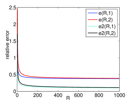
Figure 1: Relative error plot. $R$ denotes the diameter of a network, $e,e2$ denote the relative errors of random ball coverage algorithm and twice-random ball coverage algorithm.

3 Conclusion and discussion

In this paper, we strictly present the upper bound of the relative error of random ball coverage method in fractal network dimension calculation. And we also yield a simple relative error upper bound $\log_{\frac{R}{m}}2$ of twice-random ball coverage method. For many real-world networks, when the network diameter is sufficient enough this kind of relative error upper bound will tend to $0$. Therefore, if the network is sufficient enough, twice-random ball coverage is equivalent to the leat box number coverage in fractal dimension calculation and calculating fractal network dimension is not a NP-hard problem. For the networks which is not sufficient enough, we can calculate random ball number many times and get the dimension, which is also very effective and accuracy.

The above discussions can lead another problem naturally. We also can define random full box coverage. A full box with diameter $r$ is a set of nodes, such that any other nodes out of the box is added to the box will make the box diameter larger or equal to $r$. The random full box coverage algorithm with diameter $r$ can be defined as[6]: at each step we randomly choose a uncovered node $p$ as the first node of the box, and select the uncovered nodes to the box until the box become full. We guess the random full box coverage algorithm is equivalent to the least box number covering algorithm in statistic sense. In the future we will do some deep researches about this problem.

References

- [1] R. Albert, A.-L. Barabasi, Rev. Mod. Phys. 74, 47 (2002).
- [2] M. E. J. Newman, SIAM Rev. 45, 167-256 (2003).
- [3] S. Boccaletti, V.Latora, Y. Moreno, M. Chavez, and D.-U. Hwang, Physics Report. 424, 175-308 (2006).
- [4] Song C, Havlin S and Makse H A, Nature 433 392 (2005).
- [5] Song C, Havlin S and Makse H A, Nature Physics 2 275 (2006).
- [6] C. Song, L. K. Gallos, S. Havlin and H. A. Makse,J. Stat. Mech.P03006 (2007).
- [7] J. S. Kim, K.-I. Goh, B. Kahng, and D. Kim. arXiv:cond-mat/0701504 (2007).
- [8] H. Jeong, B. Tombor, R. Albert, Z. N. Oltvai and A.-L. Barabasi, Nature 407 651-654, (2000).
- [9] W. X. Zhou, Z. Q. Jiang, D.r Sornette. arXiv:cond-mat/0605676 (2006).