Rare $B_{c}\rightarrow D_{s}\ell^{+}\ell^{-}$decay beyond the standard model

The rare $B_{c}\rightarrow D_{s}\ell^{+}\ell^{-}$decay is investigated by using the most general model independent effective Hamiltonian. The general expressions of longitudinal, normal and transversal polarization asymmetries for $\ell^{-}$ and $\ell^{+}$ and the combined asymmetries of them are found. The dependencies of the branching ratios and polarizations on the new Wilson coefficients are presented. The analysis shows that the branching ratios and the lepton polarization asymmetries are very sensitive to the scalar and tensor type interactions. These results will be very useful in searching new physics beyond the standard model.

1 Introduction

Investigation of rare $B$ meson decays, induced by flavor–changing neutral current (FCNC) $b\rightarrow s,d$ [1] transitions, is an important source of new physics. These transitions take place at loop level in the SM so they can be used to test the gauge structure of the SM and provide a suitable tool of looking for new physics. In rare B meson decays, new physics contributions may appear in two different ways; modifying Wilson coefficients in the SM or adding new structures in the SM effective Hamiltonian.

Since the CLEO observation of $b\rightarrow s\,\gamma$ process [2], decays of $B_{u,d,s}$ mesons have been the subject of many investigations. These studies will be even more complete if similar studies for $B_{c}$, discovered by CDF Collaboration [3], are also included.

In the mean time, the study of the $B_{c}$ meson is by itself quite interesting too, since it has some outstanding features [4]–[6] . It is the lowest bound state of two heavy quarks ($b$ and $c$) with explicit flavor that can be compared with the charmonium ($c\bar{c}$- bound state) and bottomium ($b\bar{b}$- bound state) which have implicit flavor. The implicit-flavor states decay strongly and electromagnetically whereas the $B_{c}$ meson decays weakly. The major difference between the weak decay properties of $B_{c}$ and $B_{u,d,s}$ is that those of the latter ones are described very well in the framework of the heavy quark limit, which gives some relations between the form factors of the physical process. In case of $B_{c}$ meson, the heavy flavor and spin symmetries must be reconsidered because both $b$ and $c$ are heavy.

On the experimental side, like the running B factories in KEK and SLAC, also encourages the study of the rare B meson decays and most of the rare $B_{c}$ decays are believed to be accessible in future experiments at hadronic colliders, such as the LHC-B. The Tevatron experiments see around 100 $B_{c}$ semileptonic decays and a luminosity upgrade by a factor of ten is discussed for 2013. Atlas and CMS experiments will have more $B_{c}$ but there will be more background. This scene may not be hopeful for understanding $B_{c}$. On the other side, rapid progress on experimental techniques are still encouraging.

Measurement of the lepton polarization is an efficient way in establishing the new physics beyond the SM [7]–[15]. In this work we present a study of the branching ratio and lepton polarizations in the exclusive $B_{c}\rightarrow D_{s}\ell^{+}\ell^{-}$$~{}(\ell=\mu,~{}\tau)$ decay for a general form of the effective Hamiltonian including all possible form of interactions in a model independent way without forcing concrete values for the Wilson coefficients corresponding to any specific model. To make predictions about such an exclusive decay, one requires the additional knowledge about form factors, i.e., the matrix elements of the effective Hamiltonian between initial and final meson states. This problem, being a part of the nonperturbative sector of QCD, lacks a precise solution. In literature there are a number of different approaches to calculate the decay form factors of $B_{c}\rightarrow D_{s}\ell^{+}\ell^{-}$decay such as light front, constituent quark models, and a relativistic quark model proposed in [16]. In this work we will use the weak decay form factors calculated in [16].

The work is organized as follows. In section 2, we derive the matrix element starting from the effective Hamiltonian for the quark level process and using the appropriate form factors. Then, we present the model independent expressions for the longitudinal, transversal and normal polarizations of leptons and combined lepton-antilepton asymmetries. We give our numerical results and discussion in section 3.

2 Effective Hamiltonian and Lepton Polarizations

The $B_{c}\rightarrow D_{s}\ell^{+}\ell^{-}$decay is described at the quark level by the $b\rightarrow s\ell^{+}\ell^{-}$ transition in the standard effective Hamiltonian approach. This Hamiltonian includes all possible terms calculated independent of any models. The effective Hamiltonian for this process can be written in terms of twelve model independent four-Fermi interactions, as follows[17]:

$${\cal H}_{eff} = \frac{G\alpha}{\sqrt{2}\pi}V_{ts}V_{tb}^{\ast}\Bigg{\{}C_{SL}\,\bar{s}i\sigma_{\mu\nu}\frac{q^{\nu}}{q^{2}}\,L\,b\,\bar{\ell}\gamma^{\mu}\ell+C_{BR}\,\bar{s}i\sigma_{\mu\nu}\frac{q^{\nu}}{q^{2}}\,R\,b\,\bar{\ell}\gamma^{\mu}\ell$$

$$+ C_{LL}^{tot}\,\bar{s}_{L}\gamma_{\mu}b_{L}\,\bar{\ell}_{L}\gamma^{\mu}\ell_{L}+C_{LR}^{tot}\,\bar{s}_{L}\gamma_{\mu}b_{L}\,\bar{\ell}_{R}\gamma^{\mu}\ell_{R}+C_{RL}\,\bar{s}_{R}\gamma_{\mu}b_{R}\,\bar{\ell}_{L}\gamma^{\mu}\ell_{L}$$

$$+ C_{RR}\,\bar{s}_{R}\gamma_{\mu}b_{R}\,\bar{\ell}_{R}\gamma^{\mu}\ell_{R}+C_{LRLR}\,\bar{s}_{L}b_{R}\,\bar{\ell}_{L}\ell_{R}+C_{RLLR}\,\bar{s}_{R}b_{L}\,\bar{\ell}_{L}\ell_{R}$$

$$+ C_{LRRL}\,\bar{s}_{L}b_{R}\,\bar{\ell}_{R}\ell_{L}+C_{RLRL}\,\bar{s}_{R}b_{L}\,\bar{\ell}_{R}\ell_{L}+C_{T}\,\bar{s}\sigma_{\mu\nu}b\,\bar{\ell}\sigma^{\mu\nu}\ell$$

$$+ iC_{TE}\,\epsilon^{\mu\nu\alpha\beta}\bar{s}\sigma_{\mu\nu}b\,\bar{\ell}\sigma_{\alpha\beta}\ell\Bigg{\}}~{},$$

where $L={1-\gamma_{5}}/{2}$ and $R={1+\gamma_{5}}/{2}$ are the chiral projection operators and $C_{X}$ are the coefficients of the four–Fermi interactions. The coefficients $C_{SL}$ and $C_{BR}$ are the nonlocal Fermi interactions corresponding to $-2m_{s}C_{7}^{eff}$ and $-2m_{b}C_{7}^{eff}$ in the SM, respectively. The $C_{LL}$, $C_{LR}$, $C_{RL}$ and $C_{RR}$ terms are the vector type interactions, two of which are vector interactions containing $C_{LL}^{tot}$ and $C_{LR}^{tot}$ do already exist in the SM in combinations of the form $(C_{9}^{eff}-C_{10})$ and $(C_{9}^{eff}+C_{10})$. Therefore, we write

$$C_{LL}^{tot} = C_{9}^{eff}-C_{10}+C_{LL}~{},$$

$$C_{LR}^{tot} = C_{9}^{eff}+C_{10}+C_{LR}~{},$$

so that that $C_{LL}^{tot}$ and $C_{LR}^{tot}$ describe the sum of the contributions from SM and new physics. The terms with coefficients $C_{LRLR}$, $C_{RLLR}$, $C_{LRRL}$ and $C_{RLRL}$ describe the scalar type interactions and the last two terms, $C_{T}$ and $C_{TE}$, describe the tensor type interactions.

Having the general form of four–Fermi interaction for the $b\rightarrow s\ell^{+}\ell^{-}$ transition, the next task is to calculate the matrix element for the $B_{c}\rightarrow D_{s}\ell^{+}\ell^{-}$decay which can be expressed in terms of the invariant form factors over $B_{c}$ and $D_{s}$. These form factors are weak decay form factors [16].

$$\left<D_{s}(p_{D_{s}})\left|\bar{s}i\sigma_{\mu\nu}q^{\nu}b\right|B_{c}(p_{B_{c}})\right> = -\frac{F_{T}}{m_{B_{c}}+m_{D_{s}}}\left[{(P_{B_{c}}+P_{D_{s}})}_{\mu}q^{2}-q_{\mu}(m^{2}_{B_{c}}-m^{2}_{D_{s}})\right],$$ (2)

$$\left<D_{s}(p_{D_{s}})\left|\bar{s}\gamma_{\mu}b\right|B_{s}(p_{B_{c}})\right> = F_{+}(q^{2}){(P_{B_{c}}+P_{D_{s}})}_{\mu}+F_{-}(q^{2})q_{\mu}~{},$$ (3)

$$\left<D_{s}(p_{D_{s}})\left|\bar{s}b\right|B_{s}(p_{B_{c}})\right> = F_{-}\frac{q^{2}}{m_{b}-m_{s}}+F_{+}\frac{m^{2}_{B_{c}}-m^{2}_{D_{s}}}{m_{b}-m_{s}}~{},$$ (4)

and

$$\left<D_{s}(p_{D_{s}})\left|\bar{s}\sigma_{\mu\nu}b\right|B_{s}(p_{B_{c}})\right>=i\frac{F_{T}}{m_{B_{c}}+m_{D_{s}}}\left[{(P_{B_{c}}+P_{D_{s}})}_{\mu}q_{\nu}-q_{\mu}{(P_{B_{c}}+P_{D_{s}})}_{\nu}\right]~{},$$ (5)

where $q=p_{B_{c}}-p_{D_{s}}$ is the momentum transfer.

We can write the matrix element of the $B_{c}\rightarrow D_{s}\ell^{+}\ell^{-}$decay using Eq. (2)-(5) as

$${\cal M}(B_{c}\rightarrow D_{s}\ell^{+}\ell^{-}) = \frac{G\alpha}{4\sqrt{2}\pi}V_{tb}V_{ts}^{\ast}\Bigg{\{}\bar{\ell}\gamma^{\mu}\ell\,\Big{[}A(P_{B_{c}}+P_{D_{s}})_{\mu}+Bq_{\mu}\Big{]}$$ (6)

$$+\bar{\ell}\gamma^{\mu}\gamma_{5}\ell\,\Big{[}C(P_{B_{c}}+P_{D_{s}})_{\mu}+Dq_{\mu}\Big{]}+\bar{\ell}\ell Q+\bar{\ell}\gamma_{5}\ell N$$

$$+4\bar{\ell}\sigma^{\mu\nu}\ell(iG)\Big{[}(P_{B_{c}}+P_{D_{s}})_{\mu}q_{\nu}-(P_{B_{c}}+P_{D_{s}})_{\nu}+q_{\mu}\Big{]}$$

$$+4\bar{\ell}\sigma_{\alpha\beta}\ell\epsilon^{\mu\nu\alpha\beta}H\Big{[}(P_{B_{c}}+P_{D_{s}})_{\mu}q_{\nu}-(P_{B_{c}}+P_{D_{s}})_{\nu}q_{\mu}\Big{]}\Bigg{\}}~{},$$

where

$$A = (C_{LL}^{tot}+C_{LR}^{tot}+C_{RL}+C_{RR})F_{+}(q^{2})-2(C_{SL})+C_{BR})\frac{F_{T}}{m_{B_{c}}+m_{D_{s}}}~{},$$

$$B = (C_{LL}^{tot}+C_{RL}^{tot}+C_{RL}+C_{RR})F_{-}(q^{2})+2(C_{SL}+C_{BR})F_{T}\frac{(m_{B_{c}}-m_{D_{s}})}{q^{2}}~{},$$

$$C = (C_{LR}^{tot}+C_{RR}-C_{LL}^{tot}-C_{RL})F_{+}(q^{2})~{},$$

$$D = (C_{LR}^{tot}+C_{RR}-C_{LL}^{tot}-C_{RL})F_{-}(q^{2})~{},$$

$$Q = (C_{LRLR}+C_{RLLR}+C_{LRRL}+C_{RLRL})\Big{[}F_{-}\frac{q^{2}}{m_{b}-m_{s}}+F_{+}\frac{m^{2}_{B_{c}}-m^{2}_{D_{s}}}{m_{b}-m_{s}}\Big{]}~{},$$

$$N = (C_{LRLR}+C_{RLLR}-C_{LRRL}-C_{RLRL})\Big{[}F_{-}\frac{q^{2}}{m_{b}-m_{s}}+F_{+}\frac{m^{2}_{B_{c}}-m^{2}_{D_{s}}}{m_{b}-m_{s}}\Big{]}~{},$$

$$G = -C_{T}\frac{F_{T}}{m_{B_{c}}+m_{D_{s}}}~{},$$

$$H = -C_{TE}\frac{F_{T}}{m_{B_{c}}+m_{D_{s}}}~{}.$$ (7)

In order to calculate the final lepton polarizations, we define the orthogonal unit vector $S_{i}^{-\mu}$ in the rest frame of $\ell^{-}$ and $S_{i}^{+\mu}$ in the rest frame of $\ell^{+}$ and the polarization of the leptons along the longitudinal ($L$), transversal ($T$) and normal ($N$) directions, as done before [7, 17], by

$$S_{L}^{-\mu} \equiv (0,\vec{e}_{L}^{\,-})=\left(0,\frac{\vec{p}_{-}}{\left|\vec{p}_{-}\right|}\right)~{},$$

$$S_{N}^{-\mu} \equiv (0,\vec{e}_{N}^{\,-})=\left(0,\frac{\vec{p}\times\vec{p}_{-}}{\left|\vec{p}\times\vec{p}_{-}\right|}\right)~{},$$

$$S_{T}^{-\mu} \equiv (0,\vec{e}_{T}^{\,-})=\left(0,\vec{e}_{N}^{\,-}\times\vec{e}_{L}^{\,-}\right)~{},$$ (8)

$$S_{L}^{+\mu} \equiv (0,\vec{e}_{L}^{\,+})=\left(0,\frac{\vec{p}_{+}}{\left|\vec{p}_{+}\right|}\right)~{},$$

$$S_{N}^{+\mu} \equiv (0,\vec{e}_{N}^{\,+})=\left(0,\frac{\vec{p}\times\vec{p}_{+}}{\left|\vec{p}\times\vec{p}_{+}\right|}\right)~{},$$

$$S_{T}^{+\mu} \equiv (0,\vec{e}_{T}^{\,+})=\left(0,\vec{e}_{N}^{\,+}\times\vec{e}_{L}^{\,+}\right)~{},$$

where $\vec{p}_{\pm}$ and $\vec{p}$ are the three momenta of $\ell^{\pm}$ and $D_{s}$ meson in the center of mass (CM) frame of the lepton pair system, respectively. The longitudinal unit vectors $S_{L}^{-}$ and $S_{L}^{+}$ are boosted to the CM frame of $\ell^{+}\ell^{-}$ by Lorentz transformation,

$$S^{-\mu}_{L,\,CM} = \left(\frac{\left|\vec{p}_{-}\right|}{m_{\ell}},\frac{E_{\ell}\,\vec{p}_{-}}{m_{\ell}\left|\vec{p}_{-}\right|}\right)~{},$$

$$S^{+\mu}_{L,\,CM} = \left(\frac{\left|\vec{p}_{-}\right|}{m_{\ell}},-\frac{E_{\ell}\,\vec{p}_{-}}{m_{\ell}\left|\vec{p}_{-}\right|}\right)~{},$$ (9)

while vectors of perpendicular directions are not changed by boost.

As $\vec{n}^{\,\pm}$ being any spin direction of the $\ell^{\pm}$, in the rest frame of the leptons, the differential decay rate of the $B_{c}\rightarrow D_{s}\ell^{+}\ell^{-}$decay can be written in the following form:

$$\frac{d\Gamma(\vec{n}^{\pm})}{ds}=\frac{1}{2}\left(\frac{d\Gamma}{ds}\right)_{0}\Bigg{[}1+\Bigg{(}P_{L}^{\pm}\vec{e}_{L}^{\,\pm}+P_{N}^{\pm}\vec{e}_{N}^{\,\pm}+P_{T}^{\pm}\vec{e}_{T}^{\,\pm}\Bigg{)}\cdot\vec{n}^{\pm}\Bigg{]}.$$ (10)

Here, $s=q^{2}/m_{B_{c}}^{2}$, the superscripts ⁺ and ^- correspond to the $\ell^{+}$ and $\ell^{-}$ cases and $(d\Gamma/ds)_{0}$ corresponds to the unpolarized decay rate, whose explicit form is

$$\left(\frac{d\Gamma}{ds}\right)_{0} = \frac{G^{2}\alpha^{2}m_{B_{c}}}{2^{14}\pi^{5}}\left|V_{tb}V_{ts}^{\ast}\right|^{2}\sqrt{\lambda}v\Delta$$ (11)

where

$$\Delta = \frac{1024}{3}sv^{2}\lambda m_{B_{c}}^{6}\left|H\right|^{2}+\frac{256}{3}s(3-2v^{2})\lambda m_{B_{c}}^{6}\left|G\right|^{2}-\frac{4}{3}(v^{2}-3)\lambda m_{B_{c}}^{4}\left|A\right|$$ (12)

$$- 128m_{\ell}\lambda m_{B_{c}}^{4}Re(AG^{*})+32(1-r)m_{\ell}^{2}m_{B_{c}}^{2}Re(CD^{*})+16sm_{\ell}m_{B_{c}}^{2}\left|D\right|^{2}$$

$$+ 4sm_{B_{c}}^{2}\left|N\right|^{2}+\frac{4}{3}m_{B_{c}}^{4}s[2\lambda-(1-v^{2})(2\lambda-3(1-r)^{2})]\left|C\right|^{2}$$

$$+ 16(1-r)m_{\ell}m_{B_{c}}^{2}Re(CN^{*})+16sm_{\ell}m_{B_{c}}^{2}Re(DN^{*})+4sv^{2}m_{B_{c}}^{2}\left|Q\right|^{2}$$

and $\lambda=1+r^{2}+s^{2}-2r-2s-2rs$, $r=m_{D_{s}}^{2}/m_{B_{c}}^{2}$ and lepton velocity is $v=\sqrt{1-{4m_{\ell}^{2}}/{q^{2}}}$.

The polarizations $P_{L}^{\pm}$, $P_{T}^{\pm}$ and $P_{N}^{\pm}$ in Eq. (10) are defined by

$$P_{i}^{\pm}(q^{2})=\frac{\displaystyle{\frac{d\Gamma}{dq^{2}}(\vec{n}^{\pm}=\vec{e}_{i}^{\,\pm})-\frac{d\Gamma}{dq^{2}}(\vec{n}^{\pm}=-\vec{e}_{i}^{\,\pm})}}{\displaystyle{\frac{d\Gamma}{dq^{2}}(\vec{n}^{\pm}=\vec{e}_{i}^{\,\pm})+\frac{d\Gamma}{dq^{2}}(\vec{n}^{\pm}=-\vec{e}_{i}^{\,\pm})}}~{},$$

for $i=L,~{}N,~{}T$. Here, $P_{L}^{\pm}$ and $P_{T}^{\pm}$ represent the longitudinal and transversal asymmetries of the charged lepton $\ell^{\pm}$ in the decay plane and $P_{N}^{\pm}$ is the normal component to both of them. After calculations, the longitudinal polarization of the $\ell^{\pm}$ is

$$P_{L}^{\pm}=\frac{8m_{B_{c}}^{2}v}{\Delta}\Big{[}\mp\frac{2}{3}m_{B_{c}}^{2}\lambda Re(AC^{*})\pm\frac{16}{3}m_{B_{c}}^{2}m_{\ell}\lambda Re(CG^{*})-\frac{32}{3}m_{B_{c}}^{2}m_{\ell}\lambda Re(AH^{*})$$

$$-2m_{\ell}(1-r)Re(CQ^{*})+\frac{128}{3}m_{B_{c}}^{4}\lambda sRe(GH^{*})-2m_{\ell}sRe(DQ^{*})-sRe(NQ^{*})\Big{]}$$ (13)

where $\Delta$ is given in Eq. (12).

In a similar way, we find the transverse polarization $P_{T}^{\pm}$

$$P_{T}^{\pm}=\frac{2m_{B_{c}}^{3}\pi\sqrt{s\lambda}}{\Delta}\Big{[}\pm\frac{2}{s}m_{\ell}(1-r)Re(AC^{*})\pm\frac{32}{s}m_{\ell}^{2}(1-r)Re(CG^{*})\mp 2m_{\ell}Re(AD^{*})$$

$$\pm 32m_{\ell}^{2}Re(DG^{*})\mp Re(AN^{*})\pm 16m_{\ell}Re(GN^{*})+v^{2}Re(CQ^{*})\Big{]},$$ (14)

In the limit of $m_{\ell}\rightarrow 0$, the transverse polarization is due the scalar terms. This can give new information about new physics.

Finally, the normal polarization $P_{N}^{\pm}$ is given by

$$P_{N}^{\pm}=\frac{2m_{B_{c}}^{3}\pi v\sqrt{s\lambda}}{\Delta}\Big{[}-2m_{\ell}Im(CD^{*})-Im(CN^{*})\pm Im(AQ^{*})\mp 16m_{\ell}Im(GQ^{*})\Big{]}.$$ (15)

In this work we assume all form factors and all new Wilson coefficients are real. Therefore, the only contribution to $P_{N}^{\pm}$ in Eq. (15) comes from $\pm Im(AQ)$ term since only the function A has an imaginary part coming from $C_{9}^{eff}$. For this reason, $P_{N}^{-}=P_{N}^{+}=0$ in the SM and scalar terms in $Q$ makes normal polarization nonzero beyond the SM. This observable result gives useful clue about new physics.

Since in the SM $P_{L}^{-}+P_{L}^{+}=0$, $P_{T}^{-}-P_{T}^{+}\approx 0$ and $P_{N}^{-}+P_{N}^{+}=0$, combined analysis of the lepton and antilepton polarizations can be another useful source of new physics [17].

Using Eq. (2) we get combined longitudinal polarization

$$P_{L}^{-}+P_{L}^{+}=\frac{16m^{2}_{B_{c}}v}{3\Delta}\Big{[}128s\lambda m^{4}_{B_{c}}Re(GH^{*})-32m_{\ell}m^{2}_{B_{c}}\lambda Re(AH^{*})$$

$$-3sRe(NQ^{*})-6(1-r)m_{\ell}Re(CQ^{*})-6m_{\ell}sRe(DQ^{*})\Big{]},$$ (16)

and combined transversal polarization is the difference of the lepton and antilepton polarizations and can be calculated from Eq. (2)

$$P_{T}^{-}-P_{T}^{+}=\frac{4m^{3}_{B_{c}}\pi\sqrt{s\lambda}}{\Delta}\Big{[}-\frac{32m^{2}_{\ell}(1-r)}{s}Re(CG^{*})+\frac{2m_{\ell}(1-r)}{s}Re(AC^{*})$$

$$+2m_{\ell}Re(AD^{*})-32m^{2}_{\ell}Re(DG^{*})+Re(AN^{*})-16m_{\ell}Re(GN^{*})\Big{]}.$$ (17)

The terms containing the SM contribution to the $P_{L}^{-}+P_{L}^{+}$ in Eq. (2), completely cancel so that any nonzero measurement of this value in the experiments will provide essential evidence of new physics beyond SM. The combined normal polarization, $P_{N}^{-}+P_{N}^{+}$, is zero beyond the SM, since $P_{N}^{-}$ and $P_{N}^{+}$ receive contribution only from $Im(AQ)$ term with opposite sign.

A last note before going into details of numerical analysis is in order. In the expressions of the lepton polarizations we note that they all depend on $s$ and the new Wilson coefficients. Because of experimental difficulties of studying the polarizations of each lepton depending on both quantities, it would be better to eliminate the dependence of the lepton polarizations on $s$, by considering the averaged forms over the allowed kinematical region. The averaged lepton polarizations are defined by

$$\left<P_{i}\right>=\frac{\displaystyle\int_{(2m_{\ell}/m_{B_{c}})^{2}}^{(1-m_{D_{s}}/m_{B_{c}})^{2}}P_{i}\frac{d{\cal B}}{ds}ds}{\displaystyle\int_{(2m_{\ell}/m_{B_{c}})^{2}}^{(1-m_{D_{s}}/m_{B_{c}})^{2}}\frac{d{\cal B}}{ds}ds}~{}.$$ (18)

3 Numerical analysis and discussion

Before going on our numerical analysis of the branching ratios and the averaged polarization asymmetries $<P^{-}_{L}>$, $<P^{-}_{T}>$ and $<P^{-}_{N}>$ of $\ell^{-}$ for the $B_{c}\rightarrow D_{s}\ell^{+}\ell^{-}$decays with $\ell=\mu,\tau$ as well as the lepton-antilepton combined asymmetries $<P^{-}_{L}+P^{+}_{L}>$ and $<P^{-}_{T}-P^{+}_{T}>$, let us first introduce the input parameters used in this work:

$$m_{B_{c}}=6.50\,GeV,\,\,m_{D_{s}}=1.968\,GeV,\,\,m_{b}=4.8\,GeV,\,\,m_{\mu}=0.105\,GeV,\,\,m_{\tau}=1.77\,GeV,$$

$$|V_{tb}V^{*}_{ts}|=0.0385,\,\,\,\,\alpha^{-1}=129,\,\,G_{F}=1.17\times 10^{-5}\,GeV^{-2},$$

$$\tau_{B_{c}}=0.46\times 10^{-12}\,s,\,\,C^{eff}_{7}=-0.313,\,\,C^{eff}_{9}=4.344\,\,,C_{10}=-4.624$$ (19)

Details of the values of the individual Wilson coefficients in the SM at $\mu\sim m_{b}$ scale can be found in [15].

The given value of $C^{eff}_{9}$ corresponds only to the short-distance contributions, but we know that $C^{eff}_{9}$ also receives long-distance contributions due to conversion of the real $\bar{c}c$ into lepton pair $\ell^{+}\ell^{-}$, and they are usually absorbed into a redefinition of the short-distance Wilson coefficients:

$$C_{9}^{eff}(\mu)=C_{9}(\mu)+Y(\mu)\,\,,$$ (20)

where

$$Y(\mu) = Y_{reson}+h(y,s)[3C_{1}(\mu)+C_{2}(\mu)+3C_{3}(\mu)+C_{4}(\mu)+3C_{5}(\mu)+C_{6}(\mu)]$$

$$- \frac{1}{2}h(1,s)\left(4C_{3}(\mu)+4C_{4}(\mu)+3C_{5}(\mu)+C_{6}(\mu)\right)$$

$$- \frac{1}{2}h(0,s)\left[C_{3}(\mu)+3C_{4}(\mu)\right]$$

$$+ \frac{2}{9}\left(3C_{3}(\mu)+C_{4}(\mu)+3C_{5}(\mu)+C_{6}(\mu)\right)\,\,,$$

and $y=m_{c}/m_{b}$, and the functions $h(y,s)$ arises from the one loop contributions of the four quark operators $O_{1}$,…,$O_{6}$ explicit forms of which can be found in [18]- [20]. Parametrization of the resonance $\bar{c}c$ contribution, $Y_{reson}(s)$, given in Eq.(3) can be done by using a Breit-Wigner shape with normalizations fixed by data given in [21]

$$Y_{reson}(s) = -\frac{3}{\alpha^{2}_{em}}\kappa\sum_{V_{i}=\psi_{i}}\frac{\pi\Gamma(V_{i}\rightarrow\ell^{+}\ell^{-})m_{V_{i}}}{sm^{2}_{B}-m_{V_{i}}+im_{V_{i}}\Gamma_{V_{i}}}$$ (22)

$$\times [(3C_{1}(\mu)+C_{2}(\mu)+3C_{3}(\mu)+C_{4}(\mu)+3C_{5}(\mu)+C_{6}(\mu))]\,,$$

where the phenomenological parameter $\kappa$ is usually taken as $\sim 2.3$.

The new Wilson coefficients are the free parameters in this work, but it is possible to establish ranges out of experimentally measured branching ratios of the semileptonic rare B-meson decays

$$BR(B\rightarrow K\,\ell^{+}\ell^{-}) = (4.8^{+1.0}_{-0.9}\pm 0.3)\times 10^{-7}\,\,,$$

$$BR(B\rightarrow K^{*}\,\mu^{+}\mu^{-}) = (1.27^{+0.76}_{-0.61}\pm 0)\times 10^{-6}\,\,,$$

reported by Belle and Babar collaborations [22]-[23], also the upper bound of pure leptonic rare B-decays in the $B^{0}\rightarrow\mu^{+}\mu^{-}$ mode [24]:

$$BR(B^{0}\rightarrow\mu^{+}\mu^{-}) <1.5\times 10^{-7}\,\,.$$

All new Wilson coefficients are taken as real and varying in the region $-4\leq C_{X}\leq 4$, compliant to this upper limit and the above mentioned measurements of the branching ratios for the semileptonic rare B-decays.

The new Wilson coefficients in Eq.(2), the helicity-flipped counter-parts of the SM operators, $C_{RL}$ and $C_{RR}$, vanish in all models with minimal flavor violation in the limit $m_{s}\rightarrow 0$. However, in some MSSM scenarios there exist finite contributions from these vector operators even for a vanishing s-quark mass. In addition, scalar type interactions can also contribute through the neutral Higgs diagrams, multi-Higgs doublet models and MSSM, for some regions of the parameter spaces of the related models. In literature there are some studies to establish ranges out of constraints under various precision measurements for these coefficients (see e.g. [25]) and our choice for the range of the new Wilson coefficients are in agreement with these calculations.

To make some numerical predictions, we also need the explicit forms of the form factors $F_{+},F_{-}$ and $F_{T}$. Since there are two heavy quarks the non-relativistic effects and also the additional contributions from hard interactions might give useful information. In this work we have not considered these effects and used the results of [16], calculated in a relativistic constituent quark model in which $q^{2}$ dependencies of the form factors are given as

$$F(q^{2})=\frac{F(0)}{\Big{(}1-as+bs^{2}\Big{)}^{2}}~{},$$

where values of parameters $F(0)$, $a_{F}$ and $b_{F}$ for the $B_{c}\rightarrow D_{s}$ decay are listed in Table 1.

$$\begin{array}[]{|l|ccc|}\hline\cr&F(0)&a&b\\ \hline\cr F_{+}&\phantom{-}0.186&2.48&\phantom{-}1.62\\ F_{-}&\phantom{-}-0.190&2.44&\phantom{-}1.54\\ F_{T}&\phantom{-}0.275&2.40&\phantom{-}1.49\\ \hline\cr\end{array}$$

Table 1: $B_{c}$ meson decay form factors in a relativistic constituent quark model without impulse approximation .

Before the discussion of the results of our analysis given in a series of figures, we give our SM predictions for the longitudinal, transverse and the normal components of the lepton polarizations for $B_{c}\rightarrow D_{s}\ell^{+}\ell^{-}$decay for $\mu$ ($\tau$) channel for reference:

$$<P^{-}_{L}> = -0.8457\,(-0.1774)\,,$$

$$<P^{-}_{T}> = -0.0948\,(-0.6189)\,,$$

$$<P^{-}_{N}> = 0\,(0)\,.$$

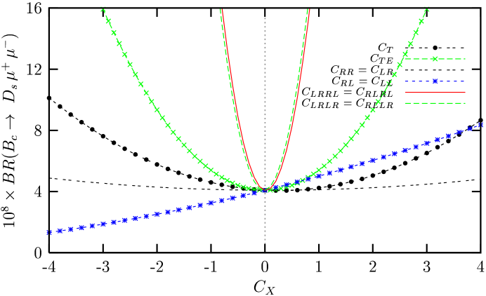
Figure 1: The dependence of the integrated branching ratio for the $B_{c}\rightarrow D_{s}\,\mu^{+}\mu^{-}$ decay on the new Wilson coefficients.

In Figs. (1) and (2), we give the dependence of the integrated branching ratio (BR) on the new Wilson coefficients for the $B_{c}\rightarrow D_{s}\mu^{+}\mu^{-}$and $B_{c}\rightarrow D_{s}\tau^{+}\tau^{-}$decays, respectively. From these figures we see that BR depends strongly on the scalar and tensor interactions and weakly on the vector interactions. It is also clear from these figures that dependence of the BR on the new Wilson coefficients is symmetric with respect to the zero point for the muon final state, but such a symmetry is not observed for the tau final state for the tensor interactions. Another remark is that, for muon case $C_{TE}$ is dominant while for tau case $C_{T}$ becomes more dominant.

In Figs. (3) and (4), we present the dependence of averaged longitudinal polarization $<P_{L}^{-}>$ of $\ell^{-}$ and the combined averaged $<P_{L}^{-}+P_{L}^{+}>$ for $B_{c}\rightarrow D_{s}\mu^{+}\mu^{-}$decay on the new Wilson coefficients. It is observed that the dominant contribution for $<P_{L}^{-}>$ comes from the scalar interactions of the type $C_{LRRL}$ and $C_{RLRL}$ which are identical and symmetric with respect to $C_{X}=0$ while the combined averaged $<P_{L}^{-}+P_{L}^{+}>$ is sensitive to that of scalar type interactions only. It is a well-known fact that vector type interactions are canceled when the longitudinal polarization asymmetry of the lepton and antilepton is considered together. This is the reason $<P_{L}^{-}+P_{L}^{+}>$ does not exhibit any vector type dependence in Fig. (4). It is also interesting to note that $<P_{L}^{-}+P_{L}^{+}>$ is positive for $C_{LRRL}$ and $C_{CRLRL}$ and negative for other scalar contributions. In addition they are symmetric with respect to $C_{X}=0$.

Figures (5) and (6) are the same as Figs. (3) and (4), but for $B_{c}\rightarrow D_{s}\tau^{+}\tau^{-}$. $<P_{L}^{-}>$ strongly depends on scalar type interactions and also sensitive to tensor type interactions. In case of vector interactions, they are nearly identical for $C_{X}>0$ and keeping their SM values. As in the muon case, $<P_{L}^{-}+P_{L}^{+}>$ depends on scalar interactions and $C_{TE}$ tensor interactions. $C_{TE}$ effect is comparably higher than that of muon case and it is negative (positive) for $C_{X}<0$ ($C_{X}>0$). For $<P_{L}^{-}+P_{L}^{+}>$ in both $\mu$ and $\tau$ decays, there is no SM effect and any nonzero experimental results of $<P_{L}^{-}+P_{L}^{+}>$ will be the evidence of new physics.

In Figs. (7) and (8), we present the dependence of averaged transverse polarization $<P_{T}^{-}>$ of $\ell^{-}$ and the combined averaged $<P_{T}^{-}-P_{T}^{+}>$ for $B_{c}\rightarrow D_{s}\ell^{+}\ell^{-}$decay on the new Wilson coefficients. The significant effect of scalar $C_{LRRL}$ and $C_{RLRL}$ can be seen from Fig. (7). Here, $<P_{T}^{-}>$ is negative (positive) for $C_{X}\stackrel{{\scriptstyle<}}{{{}_{\sim}}}0$ ($C_{X}\stackrel{{\scriptstyle>}}{{{}_{\sim}}}0$). As a last remark, all other contributions are negative except $C_{LRLR}$ and $C_{RLLR}$ scalar terms for $C_{X}\stackrel{{\scriptstyle>}}{{{}_{\sim}}}0.8$. Unlike the $<P_{T}^{-}>$, $C_{LRLR}$ and $C_{RLLR}$ make greater contribution to $<P_{T}^{-}-P_{T}^{+}>$ as seen in Fig. (8). Considering Figs. (7) and (8) together, determination of the sign and magnitude of the scalar observables can also give useful information about the existence of new physics.

Figures (9) and (10) are the same as Figs. (7) and (8), but for $B_{c}\rightarrow D_{s}\tau^{+}\tau^{-}$. In both figures, the effects of scalar contributions are clear. Considering $<P_{T}^{-}-P_{T}^{+}>$ it can be noted that values of obtained data are two times that of $<P_{T}^{-}>$ values.

Figures (11) and (12), we present the dependence of averaged normal polarization $<P_{N}^{-}>$ of $\ell^{-}$ for $B_{c}\rightarrow D_{s}\mu^{+}\mu^{-}$and $B_{c}\rightarrow D_{s}\tau^{+}\tau^{-}$decays on the new Wilson coefficients. Normal components of polarization of both channel depend only on scalar type interactions. As discussed before, SM contribution of normal polarization is zero so any measurable values should come from new physics. These values will also give promising information on sign and magnitude of $<P_{N}^{-}>$ because $<P_{N}^{-}>$ is negative (positive) for $C_{X}<0(C_{X}>0)$.

In conclusion, using the general, model independent form of the effective Hamiltonian, we present the most general analysis of the lepton polarization asymmetries in the rare $B_{c}\rightarrow D_{s}\ell^{+}\ell^{-}$decay. The dependence of the longitudinal, transversal and normal polarization asymmetries of $\ell^{-}$ and their combined asymmetries on the new Wilson coefficients are studied. The lepton polarization asymmetries are very sensitive to the existence of the scalar type interactions and in some cases tensor type interactions worth to be considered. Individually, $C_{LRRL}$ and $C_{RLRL}$ play a significant role throughout this work. In all types of analysis the following terms are found identical: $C_{RR}=C_{LR}$, $C_{RL}=C_{LL}$, $C_{LRRL}=C_{RLRL}$ and $C_{LRLR}=C_{RLLR}$. Moreover, in the most cases polarization effects change their signs as the new Wilson coefficients vary in the region of interest, which is useful to determine the sign in addition magnitude of new physics effect. A last note on combined asymmetries, a well known SM result that $<P_{L}^{-}+P_{L}^{+}>=0$, $<P_{N}^{-}+P_{N}^{+}>=0$ and $<P_{T}^{-}-P_{T}^{+}>\simeq 0$ in the limit $m_{\ell}\rightarrow 0$. Therefore any deviation from these relations and determination of the sign of polarization is decisive and effective tool in searching new physics beyond the SM.

Acknowledgments

The author would like to thank G. Turan and A. Ozpineci for valuable contributions and discussions. This work was partially supported by Mersin University under Grant No: BAP-FEF-FB (UOY) 2006-3.

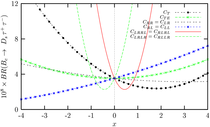
Figure 2: The dependence of the integrated branching ratio for the $B_{c}\rightarrow D_{s}\,\tau^{+}\tau^{-}$ decay on the new Wilson coefficients.

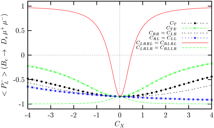
Figure 3: The dependence of the averaged longitudinal polarization $<P^{-}_{L}>$ of $\ell^{-}$ for the $B_{c}\rightarrow D_{s}\,\mu^{+}\mu^{-}$ decay on the new Wilson coefficients.

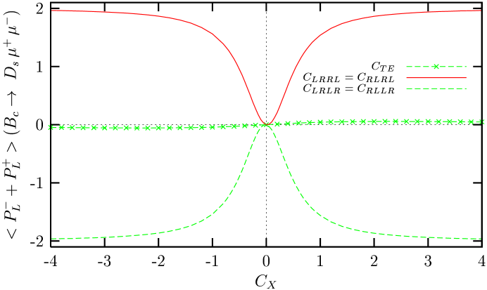
Figure 4: The dependence of the combined averaged longitudinal lepton polarization       $<P^{-}_{L}+P^{+}_{L}>$ for the $B_{c}\rightarrow D_{s}\,\mu^{+}\mu^{-}$ decay on the new Wilson coefficients.

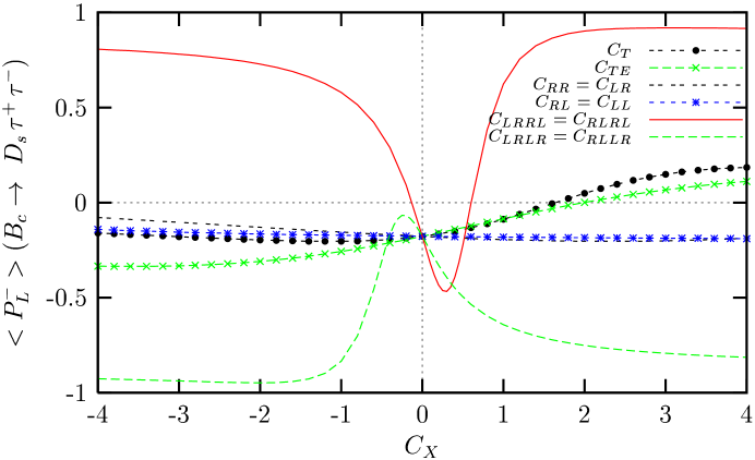
Figure 5: The same as Fig. (3), but for the $B_{c}\rightarrow D_{s}\,\tau^{+}\tau^{-}$ decay.

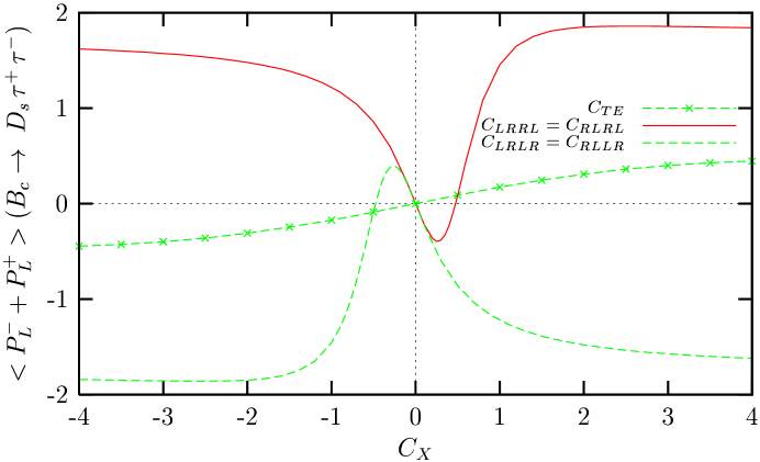
Figure 6: The same as Fig. (4), but for the $B_{c}\rightarrow D_{s}\,\tau^{+}\tau^{-}$ decay.

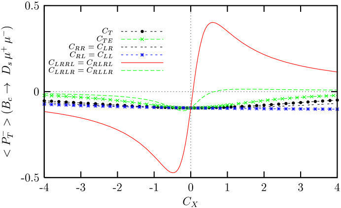
Figure 7: The dependence of the averaged transverse polarization $<P^{-}_{T}>$ of $\ell^{-}$ for the $B_{c}\rightarrow D_{s}\,\mu^{+}\mu^{-}$ decay on the new Wilson coefficients.

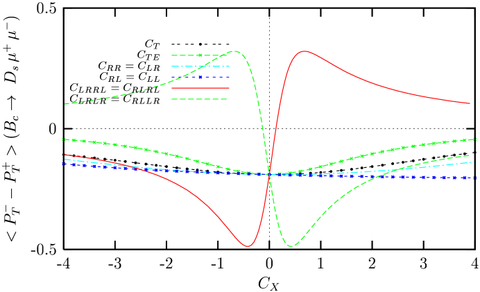
Figure 8: The dependence of the combined averaged transverse lepton polarization       $<P^{-}_{T}-P^{+}_{T}>$ for the $B_{c}\rightarrow D_{s}\gamma\,\mu^{+}\mu^{-}$ decay on the new Wilson coefficients.

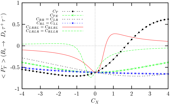
Figure 9: The same as Fig. (7), but for the $B_{c}\rightarrow D_{s}\,\tau^{+}\tau^{-}$ decay.

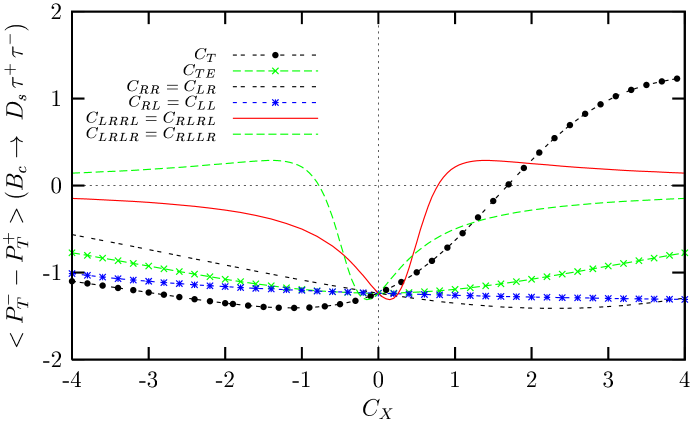
Figure 10: The same as Fig. (8), but for the $B_{c}\rightarrow D_{s}\,\tau^{+}\tau^{-}$ decay.

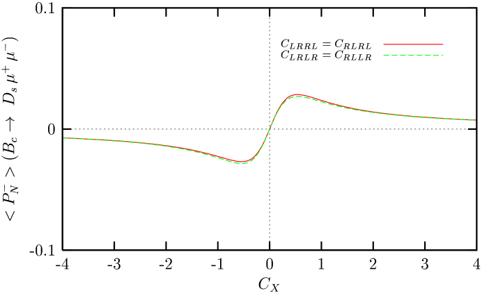
Figure 11: The dependence of the averaged normal polarization $<P^{-}_{N}>$ of $\ell^{-}$ for the $B_{c}\rightarrow D_{s}\,\mu^{+}\mu^{-}$ decay on the new Wilson coefficients.

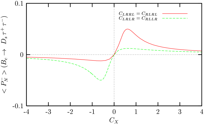
Figure 12: The same as Fig.(11), but for the $B_{c}\rightarrow D_{s}\,\tau^{+}\tau^{-}$ decay.

References

[1] A. Ali, Int. J. Mod. Phys. A 20, 5080 (2005)
[2] CLEO Collaboration, M. S. Alam, et. al., Phys. Rev. Lett. 74, 2885 (1995)
[4] P. Colangelo, F. De Fazio, Phys. Rev. D 61, 034012 (2000)
[5] M. A. Ivanov, J. G. Körner, P. Santorelli, Phys. Rev. D 63, 074010 (2001)
[6] M. A. Ivanov, J. G. Körner, P. Santorelli, Phys. Rev. D 73, 054024 (2006)
[7] F. Kruger, L. M. Sehgal, Phys. Lett. B 380, 199 (1996)
[8] Y. G. Kim, P. Ko and J. S. Lee, Nucl. Phys. B 544, 64 (1999)
[9] T. M. Aliev, M. Savci, Phys. Lett. B 481, 275 (2000)
[10] Q.-S. Yan, C. -S. Huang, L Wei, S.-H. Zhu, Phys. Rev. D 62, 094023 (2000)
[11] U. O. Yilmaz, B. B. Sirvanli, G. Turan, Nucl. Phys. B 692, 249 (2004)
[12] G. Turan, Mod. Phys. Lett. A 20, 533 (2005)
[13] T. M. Aliev, V. Bashiry, M. Savci, Phys. Rev. D 71, 035013 (2005)
[14] A. S. Cornell, N. Gaur, JHEP, 0502:005 (2005)
[15] U. O. Yilmaz, G. Turan, Eur. Phys. J. C 51, 63 (2007)
[16] A. Faessler, Th. Gutsche, M. A. Ivanov, J. G. Körner,
V. E. Lyubovitskij, Eur.Phys.J. C 4, 18 (2002)
[17] S. Fukae, C. S. Kim and T. Yoshikawa, Phys. Rev. D 61, 074015 (2000)
[18] A. J. Buras and M. Münz, Phys. Rev. D 52, 186 (1996)
[19] M. Misiak, Nucl. Phys., B 393, 23 (1993)
[20] M. Misiak, Nucl. Phys., B 439, 461 (1995) [Erratum]
[21] A. Ali, T. Mannel and T. Morozumi, Phys. Lett. B 273, 505 (1991)
[22] BELLE Collaboration, K. Abe, et al., Phys. Rev. Lett. 91, 261601 (2003)
[23] BaBar Collaboration, B. Aubert, et al., Phys. Rev. Lett. 91, 221802 (2003)
[24] CDF Collaboration, B. Abulencia, et al., Phys. Rev. Lett. 95, 221805 (2005)
[25] C.-S. Huang,X.-H. Wu, Nucl. Phys. B 665, 304
(2003)