The shadow of light: evidences of photon behaviour contradicting known electrodynamics

Abstract

We report the results of a double-slit-like experiment in the infrared range, which evidence an anomalous behaviour of photon systems under particular (energy and space) constraints. The statistical analysis of these outcomes (independently confirmed by crossing photon beam experiments in both the optical and the microwave range) shows a significant departure from the predictions of both classical and quantum electrodynamics.

1 Introduction

In the last years we carried out two optical experiments of the double-slit type, aimed at searching for a possible anomalous photon behavior, which provided strong clues for a discrepancy with the predictions of classical and/or quantum electrodynamic^(1-4). They originated from an analysis^(5,6) of the Cologne⁽⁷⁾ and Florence⁽⁸⁾ microwave experiments, which evidenced propagation of electromagnetic evanescent waves at superluminal speed. Superluminality is naturally associated to a breakdown of local Lorentz invariance (LLI), and therefore to a possible anomalous photon behavior. If evanescent waves are identified with virtual photons⁽⁹⁾, such anomalies are expected to occur within a length scale of the order of the near field size. The analysis of ref.[5] showed that the electromagnetic breakdown of LLI related to superluminal propagation of evanescent waves exhibits a threshold behavior both in energy ($E_{0,em}\simeq$4.5$\mu V$) and in space ($\ell\simeq$9 $cm$) (in the sense that it is expected to occur at energies and distances lower than the threshold values). A repetition of those interference-like experiments with a large statistics in 2005-2006 allowed us to get a definite evidence for a photon behavior contradicting standard electrodynamics, under suitable space and energy constraints.

2 Experimental setup

All the experiments were carried out at the microelectronics laboratory of L’Aquila University. The apparatus employed (schematically depicted in Fig.1) consisted of a Plexiglas box with wooden base and lid.

The box (thoroughly screened from those frequencies susceptible of affecting the measurements) contained two identical infrared (IR) LEDs, as (incoherent) sources of light, and three identical detectors (A, B, C). In all experiments the LEDS were of the kind High Speed Infrared Emitter AlGaAs (HIRL 5010, Hero Electronics Ltd.), with emission peak at 850 $nm$ and angular aperture of 20^∘.The two sources S₁, S₂ were placed in front of a screen with three circular apertures F₁, F₂, F₃ on it. The apertures F₁ and F₃ were lined up with the two LEDs A and C respectively, so that each IR beam propagated perpendicularly through each of them. The geometry of this equipment was designed so that no photon could pass through aperture F₂ on the screen. Let us stress that the apparatus was sized according to the analysis⁽⁵⁾ of the superluminal propagation experiments [7,8]. In particular, the dotted line S in Fig.1 corresponds to the horizontal distance between the planes of the horn antennas in the Florence experiment.

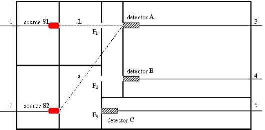
Figure 1: Above view of the experimental apparatus used in the first double-slit experiment.

The wavelength of the two photon sources was $\lambda$ = 8.5$\times$10^-5 $cm$. The apertures were circular, with a diameter of 0.5 $cm$, much larger than $\lambda$. We worked therefore in absence of single-slit (Fresnel) diffraction. However, the Fraunhofer diffraction was still present, and its effects have been taken into account in the background measurement.

Detector C was fixed in front of the source S₂; detectors A and B were placed on a common vertical panel (see Fig.1).

Let us highlight the role played by the three detectors. Detector C destroyed the eigenstates of the photons emitted by S₂. Detector B ensured that no photon passed through the aperture F₂. Finally, detector A measured the photon signal from the source S₁.

In summary, detectors B and C played a controlling role and ensured that no spurious and instrumental effects could be mistaken for the anomalous effect which had to be revealed on detector A. The design of the box and the measurement procedure were conceived so that detector A was not influenced by the source S₂ according to the known and officially accepted laws of physics governing electromagnetic phenomena: classical and/or quantum electrodynamics. In other words, with regards to detector A, all went as if the source S₂ would not be there at all or be always kept turned off.

In essence, the experiments just consisted in the measurement of the signal of detector A (aligned with the source S₁) in two different states of source lighting. Precisely, a single measurement on detector A consisted of two steps:

1)  Sampling measurement of the signal on A with source S₁ switched on and source S₂ off;

2)  Sampling measurement of the signal on A with both sources S₁ and S₂ on.

As already stressed, due to the geometry of the apparatus, no difference in signal on A between these two source states ought to be observed, according to either classical or quantum electrodynamics. If $A($S${}_{1}i$ S${}_{2}k)$ ($i,k=on,off$) denotes the value of the signal on A when source S₁ is in the lighting state $i$ and S₂ in the state $k$, a possible non-zero difference $\Delta A=A($S${}_{1}on$ S${}_{2}off)-A($S${}_{1}on$ S${}_{2}on)$ in the signal measured by A when source S₂ was off or on (and the signal in B was strictly null) has to be considered evidence for the searched anomalous effect.

Let us explicitly notice that the geometry of the box was critical in order to reveal the anomalous photon behavior.

3 The first two experiments

The main difference between the first two experiments was in the nature of the detectors A, B, C, which were photodiodes in the former case^(1,2) and phototransistors (of the type with a convergent lens) in the latter^(3,4) (see refs.[1-4] for technical details). Moreover, in the second experiment a right-to-left inversion was made along the bigger side of the box. Thus, it was possible to study how the phenomenon changes under a spatial parity inversion and for a different type of detector. In the first experiment the plane containing the detectors A, B was movable (the distance was varied by steps of 1 $cm$ on the whole range of 10 $cm$). This allowed us to study how the phenomenon changes with distance from the sources.

The outcomes of the first experiment were positive, namely the differences $\Delta A$ between the measured signals on detector A in the two conditions were different from zero. Moreover, the phenomenon obeyed the threshold behavior predicted by the analysis [5] of the Cologne and Florence experiments. In particular, $\Delta A$ ranged from (2.2$\pm$0.4)$\mu V$ to (2.3$\pm$0.5)$\mu V$, values well below the threshold energy $E_{0,em}$= 4.5$\mu V$ , and the anomalous effect was observed within a distance of at most 4 $cm$ from the sources. The dependence of the phenomenon on the detector-source distance highlights further the critical role of the geometry of the box in the detection of the phenomenon.

We can consider such an effect as the consequence of a ”hidden” (or virtual) interference between the photon beams of the two sources. This must be meant in the sense that something like a "virtual screening" occurred, which modified the photon-photon cross section thus producing a change in the number of photons detected by A ("shadow of light").

The results of the second experiment confirmed those of the first one. The value of the difference measured on detector A was (0.008$\pm$0.003)$\mu V$, which is consistent, within the error, with the difference $\Delta A$ $\simeq$ 2.3 $\mu V$ measured in the first experiment, provided that the unlike efficiencies of the phototransistors with respect to those of the photodiodes are taken into account.

The consistency between the results of the first two experiments shows apparently that the effect is not affected by the parity of the equipment and by the type of detector used (at least for photodiodes and phototransistors).

Furthermore, a different time procedure to sample the signals on the detectors was used in the two experiments. We indeed realized that the sampling time procedure was apparently crucial in order to observe the anomalous interference effect. This is due to the fact that the phenomenon has a peculiar time structure that makes the sampling procedure critical⁽³⁾. Therefore, in order to optimize the performance of the effect detection for different detectors, statistics being equal, it was necessary to suitably change the time sampling. This latter consisted of two time steps, namely the waiting time $t_{w}$ (defined as the time interval between the lighting of the source(s) and the start of the sampling on the detectors), and the measurement time $t_{m}$, i.e. the actual interval during which measurements were taken. In the first experiment, it was $t_{w}$=60 $s$ and $t_{m}$ was determined manually, whereas in the second one it was $t_{w}=1s$ and $t_{m}$ =5 $s$. Then, it turned out that there was apparently a sort of unavoidable bond between detector and sampling-time procedure, to be taken into account in order to reveal the effect.

We stress that the results of the double-slit experiments have been independently supported by experiments with orthogonal crossing photon beams, in which similar anomalous effects have been observed. We refer to two interference experiments (carried out after our first one), one with microwaves emitted by horn antennas, at IFAC - CNR (Ranfagni and coworkers)^(10,11), and the other with infrared CO₂ laser beams, at INOA-CNR (Meucci and coworkers)^(3,12).

4 Third experiment

The third experiment was planned and carried out in order to obtain a further evidence of the observed effect, by clarifying some of its features. In order to test the apparent bond between detectors and sampling time procedures, the experiment was carried out by means of the box with photodiodes but using the sampling-time procedure adopted with phototransistors (namely $t_{w}$= 1 $s$ and $t_{m}$ = 5 $s$). Our aim was just to put ourselves in the worst possible situation with respect to the effect detection.

Let us note that the photodiodes used as detectors in the first and third experiment were integrated to a transimpedance amplifier type OPT301 of Burr-Brown (registered Trade Mark), transducing the photocurrent signal into a voltage signal. Such a voltage, measured by means of a multimeter 34401A of Agilent, did not depend therefore on the value of the circuit resistances of the voltage measuring system.

As we shall see, the results of this third experiment were consistent with those of the two previous ones. Moreover, the measurements were repeated several times over a whole period of four months, in order to collect a fairly large amount of samples and hence have a significant statistical reproducibility of the results. Thanks to this large quantity of data, it was possible to study the distribution of the differences of signals on detector A, which is shown in Fig. 2. For clarity’s sake, we reported only the differences $\Delta A$ outside the interval $\left[-1,1\right]$, which is the interval of compatibility with zero of the values of $\Delta A$. The data of the single measurements have been suitably treated in order to get rid of the instrumental drift.

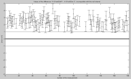
Figure 2: Value of the differences $\Delta A$ of signal sampled on detector A for the two lighting states of the sources S₁ on, S₂ off, and S₁ on, S₂ on (third experiment). The differences are clearly incompatible with zero.

We want now to show that a more detailed analysis of the measurements of the third experiment are just in favour of the anomalous interference observed as signature of a possible violation of electrodynamics.

This is easy to realize, by noting that the distribution of the results of the third experiment (reported in Fig.2) is unmistakably different from that expected from the theoretical predictions of both quantum and classical electrodynamics.

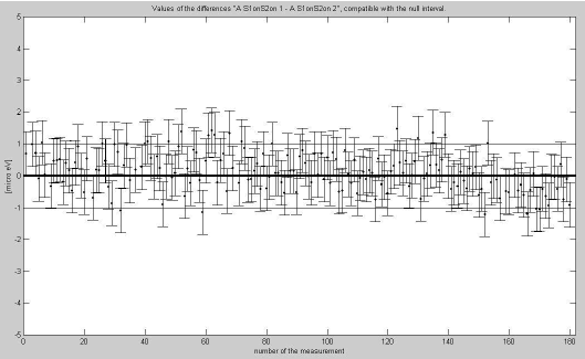
Figure 3: Values of the differences $\Delta A^{\prime}$ of signal sampled on detector A with both sources on (third experiment). The differences are clearly compatible with zero.

In this connection, let us recall that Fig.2 shows the signal differences measured on A in correspondence to the two different states of lighting of the source S₂, $\Delta A=A($S${}_{1}on$ S${}_{2}off)-A($S${}_{1}on$ S${}_{2}on)$. For comparison, we report in Fig.3 the differences of the two values sampled on A in the same lighting condition of the sources, i.e. with both sources turned on: $\Delta A^{\prime}=A($S${}_{1}on$ S${}_{2}on)-A($S${}_{1}on$ S${}_{2}on)$. For clarity’s sake, we show only the differences inside the null interval $\left[-1,1\right]$. There is no surprise in observing that the differences $\Delta A^{\prime}$ are almost evenly distributed around zero, since the subtracted values belong to the same population. However, by the very design of the experimental box, according to either classical or quantum electrodynamics detector A had not to be affected by the state of lighting of the source S₂. Hence, one would expect that the mean value of the differences $\Delta A$ (corresponding to the two different lighting states of the source S₂) was zero and that these differences were uniformly distributed around it. In other words, one would expect to find roughly the same number of positive and negative differences, and therefore that both Fig.2 and Fig.3 displayed two compatible distributions of differences evenly scattered across zero. On the contrary, the differences $\Delta A$ in Fig.2 are not uniformly distributed around zero but are markedly shifted upward (as compared to those in Fig. 3), and hence the number of positive differences is larger than the negative ones. This upward shift means that $A($S${}_{1}on$ S${}_{2}off)>A($S${}_{1}on$ S${}_{2}on)$, and hence that the signal on detector A is lower when both of the incoherent sources are on. Of course, the incoherence of sources excludes the possibility that the signal lowering could be due to destructive interference. We can conclude that distribution 3 is compatible with zero (as it must be), whereas distribution 2 is not, at variance with the predictions of either classical and quantum electrodynamics.

In order to further enforce the evidence for the difference of the two physical situations corresponding to Figs.2 and 3, we carried out a statistical analysis of the results found in the two cases (only the differences outside the interval $\left[-1,1\right]$ have been considered), by taking into account the instrumental drift. The Gaussian curves obtained are shown in Fig.4. The dashed, red curve refers to the signal differences $\Delta A=A($S${}_{1}on$ S${}_{2}off)-A($S${}_{1}on$ S${}_{2}on)$, whereas the solid, blue one to $\Delta A^{\prime}=A($S${}_{1}on$ S${}_{2}on)-A($S${}_{1}on$ S${}_{2}on)$. The two curves differ by 3.82 $\sigma$, clearly showing that the two cases are statistically distinct, the latter one representing a mere fluctuation (unlike the former). Furthermore, the mean value corresponding to the Gaussian of the differences $\Delta A$ is $\overline{\Delta A}$ = 2.41 $\mu eV$, a value in full agreement with the results of the first two experiments^(1-4).

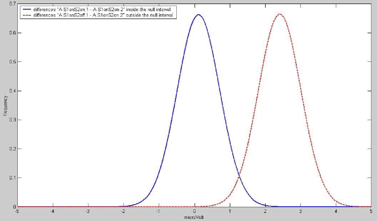
Figure 4: Gaussian curves (normal frequency vs. signal difference in $\mu V$) for the signal differences $\Delta A$ and $\Delta A^{\prime}$on detector A for the two cases of source S₂ off and on (dashed and solid curve, respectively). The instrumental drift has been taken into account. It is $\overline{\Delta A}$=2.411 ($\sigma$=0.601); $\overline{\Delta A^{\prime}}$=0.116 ($\sigma$=0.602).

As a further check, we carried out an analysis of the data of the third experiment by constraining the instrumental drift to be a constant. As is well known, such a procedure makes the observed effect to disappear if it is a mere instrumental one. On the contrary, such a strong constraint did not affect the set of data, which remains statistically significant. This means that the observed anomalous interference has not an instrumental origin.

We can therefore conclude that the results obtained on the anomalous behavior of photon systems — apparently at variance with usual (classical and quantum) electrodynamics — bring to light a more complex physics of the electromagnetic interaction, which calls for a critical reexamination of standard electrodynamics and quantum mechanics⁽⁴⁾.

Acknowledgements - Useful discussions with A. Ranfagni are gratefully acknowledged. Moreover, a special thank is due with sincere pleasure to the President of CNR Fabio Pistella, who, not only now but even previously in his capacity of President of INOA (National Institute of Applied Optics), has encouraged and supported the execution of these experiments, and has been actively involved in the discussions concerning the experimental results.

References

- [1] F. Cardone, R. Mignani, W. Perconti and R. Scrimaglio: in Proc. Int. Conf. on “Anomalies and Strange Behavior in Physics: Challenging the Conventional” (Napoli, Italy, April 10-12, 2003), D. Mugnai, A. Ranfagni and L. S. Schulman eds., Atti Fondazione G. Ronchi LVIII, n.6, 870 (2003).
- [2] F. Cardone, R. Mignani, W. Perconti and R. Scrimaglio: Phys. Lett. A 326, 1 (2004).
- [3] F. Cardone, R. Mignani, W. Perconti, A. Petrucci and R. Scrimaglio: Int. Jour. Modern Phys. B 20, 85 (2006).
- [4] F. Cardone, R. Mignani, W. Perconti, A. Petrucci and R. Scrimaglio: Int. Jour. Modern Phys. B 20, 1107 (2006).
- [5] F. Cardone and R. Mignani: Phys. Lett. A 306, 265 (2003).
- [6] F. Cardone and R. Mignani: Energy and Geometry - An Introduction to Deformed Special Relativity (World Scientific Series in Contemporary Chemical Physics, vol. 22) (World Scientific, Singapore, 2004); and references therein.
- [7] A. Enders and G. Nimtz: J. Phys. I (France) 2, 1693 (1992).
- [8] A. Ranfagni, P. Fabeni, G.P. Pazzi and D. Mugnai: Phys. Rev. E 48, 1453 (1993).
- [9] A.A Stahlhofen and G. Nimtz: Europhysics Lett. 76, 189 (2006).
- [10] A. Ranfagni, D. Mugnai and R. Ruggeri: Phys. Rev. E 69, 027601 (2004).
- [11] A. Ranfagni and D. Mugnai: Phys. Lett. A 322, 146 (2004).
- [12] D. Mugnai, A. Ranfagni, E. Allaria, R. Meucci and C. Ranfagni: Modern Phys. Lett. B19, 1 (2005).