Time-Dependent Magnetohydrodynamic Self-Similar
Extragalactic Jets

Abstract

Extragalactic jets are visualized as dynamic erruptive events modelled by time-dependent magnetohydrodynamic (MHD) equations. The jet structure comes through the temporally self-similar solutions in two-dimensional axisymmetric spherical geometry. The two-dimensional magnetic field is solved in the finite plasma pressure regime, or finite $\beta$ regime, and it is described by an equation where plasma pressure plays the role of an eigenvalue. This allows a structure of magnetic lobes in space, among which the polar axis lobe is strongly peaked in intensity and collimated in angular spread comparing to the others. For this reason, the polar lobe overwhelmes the other lobes, and a jet structure arises in the polar direction naturally. Furthermore, within each magnetic lobe in space, there are small secondary regions with closed two-dimensional field lines embedded along this primary lobe. In these embedded magnetic toroids, plasma pressure and mass density are much higher accordingly. These are termed as secondary plasmoids. The magnetic field lines in these secondary plasmoids circle in alternating sequence such that adjacent plasmoids have opposite field lines. In particular, along the polar primary lobe, such periodic plasmoid structure happens to be compatible with radio observations where islands of high radio intensities are mapped.

1 Introduction

Collimated jets with high terminal velocities appear to be universal phenomena in astrophysics. They are often associated with young stellar objects, compact galactic objects, and active galactic nuclei [Livio 1997]. These jets are always accompanied by accretion disks on the equatorial plane. The magnetosphere of the accretion disk contains a plasma that follows the accretion of the materials in the disk. The plasma density and pressure get higher as the accretion approaches to the center which drive the magnetic field. The dynamics of this system was first described in magnetohydrodynamic (MHD) model by Blandford and Payne [1982]. In this landmark paper, jets are considered as a spatial structure in stationary state. Ideal MHD equations in cylindrical coordinates $(r,\phi,z)$ are solved for time independent solutions. The central mass $M$ is replaced by a linear mass along the cylindrical axis. Self-similar solutions in space with a scale invariance $z/r$ are sought. Such self-similar solutions are compatible to a Keplerian disk plasma rotation velocity field superimposed by an Alfvénic plasma velocity. The complete MHD instability spectrum with such Keplerian profile are analysed by Keppens, Casse, and Goedbloed [2002]. This model predicts that the magnetospheric disk plasma would be ejected towards the polar direction magnetocentrifugally should the magnetic field lines be at an angle less than $\pi/3$ or more that $2\pi/3$ on the $rz$ plane with respect to the outward radius of the disk. Collimating action of this plasma outflow would be provided by the hoop force of the azimuthal magnetic field and its associated parallel current in a force-free configuration. The interaction of the magnetic field with the plasma disk generates a MHD Poynting flux [Ferreira and Pelletier 1995] that can be converted into kinetic energy of the jet plasma [Zanni et. al. 2004]. Variants of jet formation model are proposed by Contopoulos and Lovelace [1994], Contopoulos [1995], and Cao and Spruit [1994]. This accretion-ejection model provides the basic framework of current investigations of accretion disk and jets as is reviewed by Balbus and Hawley [1998]. Dissipative MHD effects are examined by Casse and Ferreira [2000 a,b] and Casse [2004], and relativistic jets are analyzed by Vlahakis [2004]. These stationary state analytic studies are often complemented by numerical works in cylindrical geometry to simulate time evolutions of the jets [Ustyugova et. al. 1995, Ouyed and Pudritz 1997, Krasnopolski et. al. 1999], and the disk-jet system [Matsumoto et. al. 1996, Kato et. al. 2002].

Here, instead of a stationary model, we take the view that jets are a time dependent spatial structure. What we see is only a snapshot of their state at this particular moment. Due to their galactic dimensions, the time scale of these structures is believed to be extraordinarily large which gives the impression of a stationary structure. This implies that jets are results of an erruption originating from the galactic nucleus. They could be dissipated in time before another erruption takes place due to pressure built-up from accretion. Or one erruption could be superimposed on an earlier event. To model the jet system, we will do a self-similar analysis on the full time-dependent ideal MHD equations in spherical coordinates $(r,\theta,\phi)$ with a mass $M$ at the nucleus. In particular, we consider axisymmetric solutions. This type of self-similar solutions were pioneered by Low [1982a,b, 1984a,b] for astrophysical applications and solar corona mass ejections with pure radial plasma velocity flow. Variants of these solutions include cases where the plasma domain lies outside the mass $M$ such as interplanetary magnetic ropes in one-dimensional [Osherovich, Farrugia, and Burlaga 1993, 1995] and in two-dimensional [Tsui and Tavares 2005] cylindrical geometry, interplanetary magnetic clouds [Tsui 2006a], and also atmospheric ball lightnings [Tsui 2006b] in spherical geometry. In these descriptions where $M$ is outside the spherical domain of interest, the magnetic field is axisymmetric force-free and contains regions of closed field lines, while the plasma is spherically symmetric decoupled from the magnetic field.

For the present case of extragalactic jets described by the mechanism of accretion-ejection, we will follow the self-similar solutions of Low with the polytropic index $\gamma=4/3$, but with particular emphasis on the finite plasma pressure. This current approach differs from the Keplerian disk plasma in that the radial flow is not tied to the Alfvén velocity as a priori. In this dynamic model, we consider jets as a manifestation of mass ejection on a galactic scale. The plasma pressure, in this self-similar MHD model, proves to have an important role in collimating the magnetic fields and the jet plasmas. The time evolution function gives a dynamic description of the high radial flow especially in the jets. The self-similar solutions, that converge at the center and at infinity, give small regions of closed axisymmetric two-dimensional magnetic field lines where plasma density and pressure are much higher. These regions along the jets could correspond to the high intensity islands in radio frequency maps.

2 Self-Similar MHD

Following the accretion-ejection classical model, we also use the MHD equations to describe the plasma. Nevertheless, we retain the time dependence to write

$${\partial\rho\over\partial t}+\nabla\cdot(\rho\vec{v})\,=\,0\,\,\,,$$

$$\rho\{{\partial\vec{v}\over\partial t}+(\vec{v}\cdot\nabla)\vec{v}\}\,=\,\vec{J}\times\vec{B}-\nabla p-\rho{GM\over r^{3}}\vec{r}\,\,\,,$$

$${\partial\vec{B}\over\partial t}\,=\,-\nabla\times\vec{E}\,=\,\nabla\times(\vec{v}\times\vec{B})\,\,\,,$$

$$\nabla\times\vec{B}\,=\,\mu\vec{J}\,\,\,,$$

$$\nabla\cdot\vec{B}\,=\,0\,\,\,,$$

$${\partial\over\partial t}({p\over\rho^{\gamma}})+(\vec{v}\cdot\nabla)({p\over\rho^{\gamma}})\,=\,0\,\,\,.$$

Here, $\rho$ is the mass density, $\vec{v}$ is the bulk velocity, $\vec{J}$ is the current density, $\vec{B}$ is the magnetic field, $p$ is the plasma pressure, $\mu$ is the free space permeability, and $\gamma$ is the polytropic index. For the bulk velocity, it is consisted of a radial and an azimuthal component to model the plasma outflow and the disk rotation. To be compatible to the physical situation, the meridian velocity is taken to be null. For the radial component $v\hat{r}$, we seek self-similar solutions where the time evolution is described by the dimensionless evolution function $y(t)$. The radial profile is time invariant in terms of the radial label $\eta=r(t)/y(t)$, which has the dimension of $r$, such that $\eta$ is independent of time, and corresponds to the Lagrangian radial position attached to a fixed fluid element. The label $\eta$ corresponds to the radial positions of the initial self-similar configuration that expands in time with radial Eulerian positions $r(t)=\eta y(t)$. The velocity can then be written as

$$\vec{v}\,=\,\{\eta{dy\over dt},0,v_{\phi}\}\,\,\,.$$

We consider a two-dimensional case with azimuthal symmetry in $\phi$. In this case, the magnetic field, through the vector potential $\vec{A}$, can be expressed in terms of two scalar functions $P$ and $Q$

$$\vec{B}\,=\,{1\over r\sin\theta}\{+{1\over r}{\partial\over\partial\theta}(rA_{\phi}\sin\theta),-{\partial\over\partial r}(rA_{\phi}\sin\theta),+\sin\theta[{\partial\over\partial r}(rA_{\theta})-{\partial\over\partial\theta}(A_{r})]\}\,$$

$$=\,{1\over r\sin\theta}\{+{1\over r}{\partial\over\partial\theta}(P),-{\partial\over\partial r}(P),+Q\}\,=\,\nabla P\times\nabla\phi+Q\nabla\phi\,\,\,.$$

We remark that the velocity field in cylindrical stationary state accretion-ejection model is a three-component field. This is necessary because the jets are generated by magnetocentrifugal motion of the planar disk plasma to the axial direction. Here, in this spherical dynamic model, the velocity field is a two-component field with $v_{\theta}=0$, because the jets are generated by first pulling the disk plasma to the center and then redirecting it to space radially through erruptions.

By self-similar solutions in time, we mean a special class of time-dependent solutions where the time and space parts of the physical quantities are in a separable form. The time part is described by the evolution function $y(t)$, and the space part will be solved self-consistently by separation of variables. The concept of self-similar dynamics is closely related to self-organized states that often have minimum energy under given constraints. Having this in mind, we now transform the independent variables from $(r,\theta,t)$ to $(\eta,\theta,y)$, and proceed to determine the explicit dependence of $y$ in each one of the physical quantities with this radial velocity. First, making use of Eq.(7), Eq.(1) renders

$${\partial\rho\over\partial t}+{1\over r^{2}}{\partial\over\partial r}(r^{2}v\rho)\,=\,({\partial\rho\over\partial t}+v{\partial\rho\over\partial r})+\rho({\partial v\over\partial r}+{2v\over r})\,=\,0\,\,\,.$$

Considering the second equality, the first bracket is the convective time derivative in Euler fluid coordinates, and this amounts to the time derivative in Lagrangian fluid coordinates. We, therefore, have

$${\partial\rho\over\partial y}{dy\over dt}+\rho({\partial v\over\partial r}+{2v\over r})\,=\,{\partial\rho\over\partial y}{dy\over dt}+{3\rho\over y}{dy\over dt}\,=\,({\partial\rho\over\partial y}+{3\rho\over y}){dy\over dt}\,=\,0\,\,\,.$$

Solving this equation for the $y$ dependence gives

$$\rho(\vec{r},t)\,=\,{1\over y^{3}}\bar{\rho}(\eta,\theta)\,\,\,.$$

As for Eq.(6), with $F=(p/\rho^{\gamma})$ it follows that

$${\partial F\over\partial t}+v{\partial F\over\partial r}\,=\,{\partial F\over\partial y}{dy\over dt}\,=\,0\,\,\,,$$

$$({p\over\rho^{\gamma}})\,=\,F(\vec{r},t)\,=\,{1\over y^{0}}\bar{F}(\eta,\theta)\,\,\,.$$

Using the representation of Eq.(8), Eq.(3) is represented by the following two equations

$${\partial P\over\partial t}+v{\partial P\over\partial r}\,=\,{\partial P\over\partial y}{dy\over dt}\,=\,0\,\,\,,$$

$${\partial Q\over\partial t}+{\partial\over\partial r}(vQ)\,=\,{\partial\over\partial r}(v_{\phi}{1\over r}{\partial P\over\partial\theta})-\sin\theta{\partial\over\partial\theta}(v_{\phi}{1\over r\sin\theta}{\partial P\over\partial r})\,\,\,.$$

The first equation gives the function $P$ as

$$P(\vec{r},t)\,=\,{1\over y^{0}}\bar{P}(\eta,\theta)\,\,\,.$$

As for the function $Q$, the right side of the second equation vanishes for rigid rotation to give

$$v_{\phi}\,=\,\omega_{0}r\sin\theta\,\,\,,$$

$${\partial Q\over\partial t}+{\partial\over\partial r}(vQ)\,=\,{\partial Q\over\partial y}{dy\over dt}+{Q\over y}{dy\over dt}\,=\,({\partial Q\over\partial y}+{Q\over y}){dy\over dt}\,=\,0\,\,\,,$$

$$Q(\vec{r},t)\,=\,{1\over y^{1}}\bar{Q}(\eta,\theta)\,\,\,.$$

We note that $v_{\phi}$ amounts to a constant plasma rotation, which has to be distinguished from the Keplerian disk rotation of the solid material. Comparing to the erruptive time scale of our dynamic approach of jets, this rotation rate is negligible and we take $\omega_{0}=0$. As for the magnetic field components, they are given by

$$B_{r}\,=\,{1\over y^{2}}\bar{B}_{r}(\eta,\theta)\,=\,+{1\over y^{2}}{1\over\eta\sin\theta}mbbbbbbb{1\over\eta}{\partial\bar{P}\over\partial\theta}\,\,\,,$$

$$B_{\theta}\,=\,{1\over y^{2}}\bar{B}_{\theta}(\eta,\theta)\,=\,-{1\over y^{2}}{1\over\eta\sin\theta}{\partial\bar{P}\over\partial\eta}\,\,\,,$$

$$B_{\phi}\,=\,{1\over y^{2}}\bar{B}_{\phi}(\eta,\theta)\,=\,+{1\over y^{2}}{1\over\eta\sin\theta}\bar{Q}\,\,\,.$$

3 Self-Organization

Before proceeding with the analysis, let us recall on the fundamentals of self-organiation, in particular on MHD systems. We note that MHD equations, like Navier-Stokes equations, have quadratic invariants in the absence of dissipations. In MHD systems, there are three of them. They are the total energy (plasma and magnetic), magnetic helicity, and cross-helicity. Because of the existence of multiple invariants, the system tends to develope self-organized and self-similar states through dissipative processes regardless of the details of the initial conditions [Hasegawa 1985]. A simple example in fluid mechanics is the developement of shock waves from an initial explosion. Another example is that fluid vortex rings (solitons) in air are often formed in fast upward drafts of smokes. Should we consider a thin layer of oil heated from below, a grid of complex highly organized hexagonal convective cells would develope regardless of the details of the initial conditions. We note that, for self-organized states, the memories of the initial conditions are lost. In other words, we can not trace a self-organized state backwards in time to its initial conditions. They are lost in the dissipative processes that lead to organization. The underlying physical arguments for self-similar solutions are also discussed in detail by Low [1982a]. For these fundamental reasons, although complex self-similar solutions are only a subset of general time-dependent MHD solutions, where most of them are not self-similar, they are prone to develope in nature with simple initial configurations.

Numerically, starting from MHD equations with any fluctuations in a given initial configuration, self-organization could be reached since they are insentive to the details in the initial conditions. Analytically, the nature of self-similarity implies that the dependent variables $(\vec{r},t)$ of a physical variable appear in separable form as we have done in Eqs.(9-14). As a consequence, the solutions will be obtained by the method of separation of variables. Naturally, this imposes severe restrictions of the physical system where such a procedure is feasible, such as the dimensionality and symmetry. Most of the self-similar solutions are established in axisymmetric systems whether cylindrical or spherical. Nevertheless, Gibson and Low [1998] have made a great leap in establishing a three-dimensional spherical solution. Under the framework of separation of variables, different kinds of solutions can be obtained for the same system depending on the choice of constants. Likewise in MHD systems, we can have different self-similar solutions to account for different phenomena depending on how we separate the constants. In the next section, we choose to solve the system with an oscillating radial solution because this solution gives magnetic toroids along the jet that match with observations. A monotonic decreasing or increasing radial solution in power form is also possible [Lynden-Bell and Boily 1994]. Although this monotonic solution is not relevant for galactic jets, it could be useful for other natural phenomena such as in two-dimensional interplanetary magnetic ropes [Tsui and Tavares 2005] and some other astrophysical objects.

4 Low Model

Comparing the equation of $F=(p/\rho^{\gamma})$ and the equation of $P$, we conclude that $F=F(P)$ is a functional of $P$ or $\bar{F}=\bar{F}(\bar{P})$. We remark that usually we can not make the above statement just based on the similarity of the governing equations. It is only possible when we are under the framework of self-similarity. We can, therefore, write the $\theta$ dependence in $\bar{\rho}$ and $\bar{p}$ in terms of $\bar{P}$ to get

$$\bar{\rho}\,=\,\bar{\rho}(\eta,\bar{P})\,\,\,,$$

$$p\,=\,{1\over y^{3\gamma}}\bar{F}(\eta,\theta)\bar{\rho}^{\gamma}(\eta,\theta)\,=\,{1\over y^{3\gamma}}\bar{F}(\bar{P})\bar{\rho}^{\gamma}(\eta,\bar{P})\,=\,{1\over y^{3\gamma}}\bar{p}(\eta,\bar{P})\,\,\,.$$

Furthermore, the $\eta$ and $\bar{P}$ dependences should be in a separable form in both

$$\bar{\rho}(\eta,\bar{P})\,=\,\bar{\rho}_{1}(\eta)\bar{\rho}_{2}(\bar{P})\,\,\,,$$

$$\bar{p}(\eta,\bar{P})\,=\,\bar{p}_{1}(\eta)\bar{p}_{2}(\bar{P})\,\,\,,$$

so that, with an adequate $\gamma$, $\bar{F}$ could come out as a functional of $\bar{P}$ only. Making use of Eq.(4) to eliminate the current density in Eq.(2), we get the momentum equation which has three components. First, we examine the $\phi$ component which contains only the magnetic force

$${\partial P\over\partial r}{\partial Q\over\partial\theta}-{\partial P\over\partial\theta}{\partial Q\over\partial r}\,=\,{1\over y^{2}}\{{\partial\bar{P}\over\partial\eta}{\partial\bar{Q}\over\partial\theta}-{\partial\bar{P}\over\partial\theta}{\partial\bar{Q}\over\partial\eta}\}\,=\,0\,\,\,,$$

$$\bar{Q}\,=\,\bar{Q}(\bar{P})\,\,\,.$$

The vanishing of the magnetic force in the azimuthal direction described by Eq.(16a) implies the functional relationship given by Eq.(16b). As for the $\theta$ component, with the knowledge of $p=\bar{p}(\eta,\bar{P})/y^{3\gamma}$, it reads

$${\partial P\over\partial\theta}\{{\partial^{2}P\over\partial r^{2}}+{1\over r^{2}}\sin\theta{\partial\over\partial\theta}({1\over\sin\theta}{\partial P\over\partial\theta})+Q{\partial Q\over\partial\theta}/{\partial P\over\partial\theta}+\mu r^{2}\sin^{2}\theta{\partial p\over\partial\theta}/{\partial P\over\partial\theta}\}\,$$

$$=\,{1\over y^{2}}{\partial\bar{P}\over\partial\theta}\{{\partial^{2}\bar{P}\over\partial\eta^{2}}+{1\over\eta^{2}}\sin\theta{\partial\over\partial\theta}({1\over\sin\theta}{\partial\bar{P}\over\partial\theta})+\bar{Q}{\partial\bar{Q}\over\partial\bar{P}}+\mu y^{4-3\gamma}\eta^{2}\sin^{2}\theta{\partial\bar{p}\over\partial\theta}/{\partial\bar{P}\over\partial\theta}\}\,=\,0\,\,\,.$$

We remark that the first three terms of this equation represent the force-free field equation for $\vec{J}\times\vec{B}=0$ [Aly 1984, Low 1986, Low and Lou 1990, Lynden-Bell and Boily 1994]. The last term is the plasma pressure. This equation would be independent of the evolution function $y$ should we consider the $\gamma=4/3$ case pioneered by Low.

We note that a nonlinear equation like Eq.(17a) has to be solved subject to the boundary conditions of a given physical problem. For example, should the problem on hand has an infinite external domain and power form radial solutions are physically reasonable, then we use fractional powers of $\bar{P}$ for the functionals of $\bar{Q}$ and $\bar{p}$ [Lynden-Bell and Boily 1994]. In our present case, we are interested in decaying oscillating solutions in $\eta$. We, therefore, write

$$\bar{Q}(\bar{P})\,=\,a\bar{P}\,\,\,,$$

$$\bar{p}(\eta,\bar{P})\,=\,\bar{p}_{1}(\eta)\bar{p}_{2}(\bar{P})\,=\,(\eta^{-4})(b^{\prime 2}\bar{P}^{2}+\bar{C})\,\,\,,$$

where $\bar{C}$ is a positive constant independent of coordinates and the functional $\bar{P}$. This is the simplest representation where the first equation gives a linear dependence of $\bar{P}$ and the second equation reflects the positive definite nature of plasma pressure. This choice of constant $\bar{C}$ in plasma pressure profile differs from the spherically symmetric radial coordinate dependent additive term in Eqs.(21) and (22) of Low [1984b]. This difference of representation stems from the view that Low considers Eq.(17a) as an equation that solves for the plasma pressure under a given $\bar{P}$. For this reason, the homogeneous solution corresponds to the spherically symmetric gasodynamic solution. We regard Eq.(17a) as an equation that solves for $\bar{P}$ under a given plasma pressure that has a positive definite separable form as in Eq.(18b). The choice of Eq.(18a) gives $\partial\bar{Q}/\partial\bar{P}=a$, a constant. With $b^{2}=2\mu b^{\prime 2}$, Eq.(17a) now reads

$$\eta^{2}{\partial^{2}\bar{P}\over\partial\eta^{2}}+\sin\theta{\partial\over\partial\theta}({1\over\sin\theta}{\partial\bar{P}\over\partial\theta})+\eta^{2}a^{2}\bar{P}+b^{2}\sin^{2}\theta\bar{P}\,=\,0\,\,\,.$$

Writing $\bar{P}(\eta,\theta)=R(\eta)\Theta(\theta)$, $x=\cos\theta$, and with $n(n+1)$ as separation constant, Eq.(17b) becomes

$$\eta^{2}{\partial^{2}R\over\partial\eta^{2}}+[a^{2}\eta^{2}-n(n+1)]R\,=\,0\,\,\,,$$

$$(1-x^{2}){d^{2}\Theta(x)\over dx^{2}}+[n(n+1)+b^{2}(1-x^{2})]\Theta(x)\,=\,0\,\,\,.$$

The $R(\eta)$ equation can be solved readily to give

$$R(\eta)\,=\,(a\eta)^{1/2}J_{n+1/2}(a\eta)\,\,\,.$$

Such a spherical Bessel functional was used by Low [1984b] in Eq.(28) of his paper as one of the numerical examples in spherical two-dimensional self-similar MHD to model coronal mass ejections.

The $\Theta(x)$ equation with finite plasma pressure, $b^{2}\neq 0$, can be solved by power series

$$\Theta(x)\,=\,\sum\,a_{m}x^{m}\,\,\,,$$

$$(m+2)(m+1)a_{m+2}=[m(m-1)-n(n+1)-b^{2}]a_{m}+b^{2}a_{m-2}\,\,\,,$$

$$6a_{3}=-[n(n+1)+b^{2}]a_{1}\,\,\,,$$

$$2a_{2}=-[n(n+1)+b^{2}]a_{0}\,\,\,,$$

where the infinite sum in Eq.(19b) starts from $m=0$. There are two independent solutions. The first one has $a_{0}=\Theta(0)\neq 0$ and $a_{1}=0$, and the second one has $a_{0}=0$ and $a_{1}=d\Theta(0)/dx\neq 0$. They correspond to even and odd powers of the series respectively

$$\Theta_{even}(x)\,=\,\sum\,a_{2m}x^{2m}\,\,\,,$$

$$\Theta_{odd}(x)\,=\,\sum\,a_{2m+1}x^{2m+1}\,\,\,.$$

In the absence of plasma pressure with $b^{2}=0$, the above solution reduces to

$$\Theta(x)\,=\,(1-x^{2}){dP_{n}(x)\over dx}\,=\,-n(n+1)\int_{1}^{x}P_{n}(x)dx\,\,\,,$$

where $P_{n}(x)$ is the Legendre polynomial. The even solution corresponds to $n$ odd, and the odd solution is otherwise.

5 Self-Similar Magnetic Field

With the solution $\bar{P}(\eta,\theta)=R(\eta)\Theta(\theta)$ established by Eqs.(19), the magnetic field components are

$$B_{r}\,=\,-{1\over y^{2}}{1\over\eta^{2}}R(\eta){d\Theta(x)\over dx}\,\,\,,$$

$$B_{\theta}\,=\,-{1\over y^{2}}{1\over\eta}{dR(\eta)\over d\eta}{1\over(1-x^{2})^{1/2}}\Theta(x)\,\,\,,$$

$$B_{\phi}\,=\,+{1\over y^{2}}{a\over\eta}R(\eta){1\over(1-x^{2})^{1/2}}\Theta(x)\,\,\,.$$

We note that the self-similar evolution of the MHD plasma distorts the dipole-like magnetic field by generating an azimuthal component of the magnetic field with finite $a^{2}$. To grasp the magnetic structure given by Eqs.(19a) and (19b), we first examine the case with $b^{2}=0$. In this special case, the even and odd power series of Eq.(19b) will terminate at a finite number of terms when $m=n+1$ to give Eq.(19b’) and $\Theta(x)=0$ at the poles $x=\pm 1$.

The self-similar radial structure $R(\eta)$ given by Eq.(19a) allows oscillations in $\eta$ if $a\eta$ is sufficiently large, which means that the azimuthal magnetic field is sufficiently large. The meridian structure $\Theta(x)$ given by Eq.(19b’) also oscillates in $x$. Let us denote $\eta_{i}$ and $x_{j}$ as where $R(\eta)$ and $\Theta(x)$ vanish. We remark that $\eta_{i}$ are circles of constant $\eta$, and $x_{j}$ are spokes of constant $x=\cos\theta$. Consequently, $(\eta_{i},x_{j})$ divide the $(\eta-x)$ plane in many smaller regions. On $\eta_{i}$, we have $B_{r}=0$ and $B_{\phi}=0$, with $B_{r}$ and $B_{\phi}$ changing signs across $\eta_{i}$. The only component that does not vanish completely on $\eta_{i}$ is $B_{\theta}$. Referring to the complete expression of $B_{\theta}$ above, this magnetic component is modulated by $\Theta(x)$ so that it changes sign on the circle of constant $\eta$ on crossing each spoke region of $x_{j}$. On $x_{j}$, we have $B_{\theta}=0$ and $B_{\phi}=0$, with $B_{\theta}$ and $B_{\phi}$ changing signs across $x_{j}$. The only component that does not vanish completely on $x_{j}$ is $B_{r}$. Referring to the complete expression of $B_{r}$ above, this magnetic component is modulated by $R(\eta)$ so that it changes sign on the spoke of constant $x$ on crossing each circular region of $\eta_{i}$. As a result, axisymmetric closed magnetic field lines are formed in these regions generating toroidal belt plasmoids circumscribing the z-axis of symmetry. We call these secondary plasmoids, and call the larger self-similar plasmoid embedding all the secondary plasmoids the primary plasmoid. Neighboring plasmoids have field lines circling in opposite sense. If one plasmoid has field lines in clockwise direction, the adjacent one has them in counter clockwise direction. The azimuthal components also rotate against each other.

In each region bounded by $(\eta_{i},\eta_{i+1})$ and $(x_{j},x_{j+1})$, the topological center defined by $dR(\eta)/d\eta=0$ and $d\Theta(x)/dx=0$ has $B_{r}=0$ and $B_{\theta}=0$. This is the magnetic axis of each toroid. The field lines about this center are given by

$${B_{r}\over dr}\,=\,{B_{\theta}\over rd\theta}\,=\,{B_{\phi}\over r\sin\theta d\phi}\,\,\,.$$

By axisymmetry, the magnetic field components are independent of $\phi$. For this reason, the third group of the above equation is decoupled from the first two groups. The $B_{\phi}$ field circles about the z-axis of symmetry without twisting. It is simply superimposed on the $B_{r}-B_{\theta}$ field lines. In terms of Fourier components $e^{im\phi}$, this means $m=0$. For the field lines on an $(r-\theta)$ plane, we consider the first equality between $B_{r}$ and $B_{\theta}$ which gives $\bar{P}=R(\eta)\Theta(x)$ equals to a constant or

$$\bar{P}(\eta,x)\,=\,(a\eta)^{1/2}J_{n+1/2}(a\eta)\Theta(x)\,=\,C\,\,\,.$$

In other words, the nested field lines are given by the contours of $\bar{P}(\eta,x)$ on the $(r-\theta)$ plane.

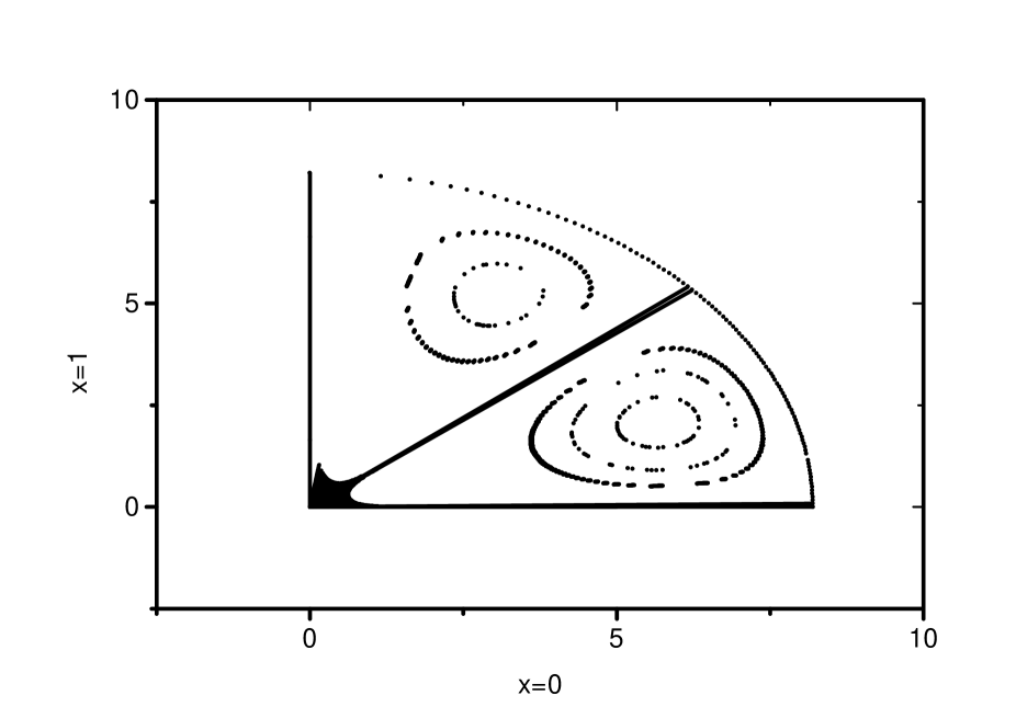
Figure 1: The field lines on the $(r-\theta)$ plane are plotted in one quadrant with $a\eta_{0}=8.2$ as the first zero of the spherical Bessel function. The quadrant is divided into two regions by $C=0$ with plasmoids having $C=-0.3,-0.5,-0.7$ and $C=+0.3,+0.5$.

As an example, the field lines for $n=4$ and $b^{2}=0$ are shown in Fig.(1) for axisymmetric secondary plasmoids. We have taken $a\eta_{0}=8.2$ at the first zero of the spherical Bessel function where $\eta_{0}$ is the radial label of the plasma boundary. The horizontal axis is $x=0$ or $\theta=\pi/2$ and the vertical axis is $x=+1$ or $\theta=0$. For $n=4$, $\Theta(x)$ vanishes at $x=0,\pm(3/7)^{1/2},\pm 1$, and $R(\eta)$ vanishes at $a\eta=0.0,8.2$. These are locations where $B_{\theta}=0$ and $B_{r}=0$ respectively dividing the quadrant in two regions, as indicated in Fig.(1). These dividing lines are obtained by solving the contours with $C=0$ numerically. The radial grids are equally spaced in $\eta$. The meridian grids are equally spaced in $x$. By converting to $\theta$ through $x=\cos\theta$, it generates an uneven grid distribution in $\theta$ that appears in Fig.(1). Closed field lines are also shown in each region. Negative value contours of $C=-0.3,-0.5,-0.7$ show the field lines in the region adjacent to the axis of $x=0$, and positive value contours of $C=+0.3,+0.5$ show the field lines in the region adjacent to the axis of $x=+1$. At the topological center of each region, we have $\Theta(x)$ maximum and $R(\eta)$ maximum, thereby giving $B_{\theta}=0$ and $B_{r}=0$ at the same location. Since

$$2\pi r\sin\theta B_{\phi}\,=\,2\pi aP\,\,\,,$$

the center has the maximum of line integral of $B_{\phi}$ about the axis of symmetry. Adjacent secondary plasmoids have oposite signs of $B_{\phi}$. Should we take $a\eta_{0}=11.7$ as the second zero of the spherical Bessel function, one additional shell of secondary plasmoids would be added to Fig.(1). Furthermore, because of the $(1-x^{2})$ factor in Eq.(19b’), $\Theta(x)$ is null at the poles with $x=\pm 1$ where the magnetic field is purely radial. If $n\gg 1$, the null at the poles is tightly surrounded by a polar lobe. Along the polar lobe, the embedded belt plasmoids are tightly wounded about the polar axis, and we name them secondary plasmoids.

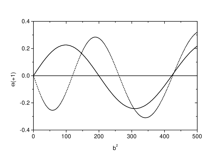
Figure 2: The function $\Theta(x)$ at $x=+1$ is plotted against the parameter $b^{2}$ to identify the eigenvalues for $n=13$ in segmented line and $n=23$ in solid line.

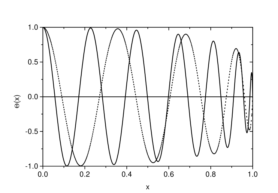
Figure 3: The eigenfunction $\Theta(x)$ is plotted against $x$ with eigenvalue $b^{2}=119$ for $n=13$ in segmented line and $b^{2}=200$ for $n=23$ in solid line to show its dependence on $n$.

We are now ready to examine the general case of $b^{2}\neq 0$. This case of $b^{2}\neq 0$ is known as the finite $\beta$ case where $\beta$ is the ratio of plasma pressure to magnetic pressure. The presence of the plasma pressure with finite $b^{2}$ distorts the linear solution of $\Theta(x)$. With finite $\beta$, the series usually has a finite value at $x=\pm 1$ which leads to singular magnetic fields there because of the $(1-x^{2})^{1/2}$ factor in the denominator. Constrained by nature to regular solutions, $b^{2}$ has to be the eigenvalues such that $\Theta(x)$ remains null at $x=\pm 1$. To search for these eigenvalues, we evaluate $\Theta(x)$, Eq.(19b), at the boundary $x=+1$ for different values of $b^{2}$ with a given $n$. The eigenvalues are shown in Fig.(2) as the intercepts of $\Theta(+1)=0$ at 119, 261, 425 for even series with $n=13$. As for $n=23$, they are 200, 422. The even series has $\Theta(0)\neq 0$ and $d\Theta(0)/dx=0$ and the odd series has $\Theta(0)=0$ and $d\Theta(0)/dx\neq 0$. The even eigenfunctions with $n=13$ and $b^{2}=119$, and with $n=23$ and $b^{2}=200$, are shown in Fig.(3). With $n=13$ and $b^{2}=119$, there are seven nodes in the inverval $(0,1)$. Should we take the second eigenvalue $b^{2}=261$, one more node would be added. With $n=23$ and $b^{2}=200$, there are twelve node in $(0,1)$. The next eigenvalue $b^{2}=422$ would add one more node as well.

The fact that the plasma pressure has to be as such that it is the eigenvalue of the $\Theta(x)$ equation appears to be a very restrictive constraint for the self-similar solutions. Nevertheless, we note that the plasma pressure appears in the $\Theta(x)$ equation where the separation constant $n(n+1)$ is an as yet unspecified free parameter. As a result, there will be an adequate $n$ for almost any given plasma pressure. For example, with $b^{2}=422$, instead of being the second eigenvalue of $n=23$, it could be the first eigenvalue of some different $n$ that is larger than 23. The important point is that for any plasma pressure $b^{2}$, it will coincide to one of the eigenvalues of some $n$. The chances are that $n$ is a large integer which, as we will show in the next section, leads to good jet collimation.

6 Jet Collimation and Vortex Structure

One important point we should point out is that, although we have taken a spherically symmetric radial expansion in the plasma velocity, the plasma density and pressure need not be symmetric, and much less the magnetic fields. The plasma profiles will be discussed later. Here, we discuss the magnetic fields that are given in terms of $R(\eta)$ and $\Theta(x)$ as listed in the preceeding section. The maximum of $\Theta(x)$ at $x=0$ gives $B_{r}=0$ on the equatorial acreation disk plasma where the magnetic field has only a $B_{\theta}$ meridian and a $B_{\phi}$ azimuthal component. Off the disk, due to the nodes in Fig.(3), there are also maxima in space, so that the magnetic fields are structured in lobes other than the equatorial lobe.

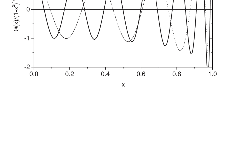
Figure 4: The function $\Theta(x)/(1-x^{2})^{1/2}$ is plotted against $x$ with eigenvalue $b^{2}=119$ for $n=13$ in segmented line and $b^{2}=200$ for $n=23$ in solid line to show the structure of $B_{\theta}$ and $B_{\phi}$ in space.

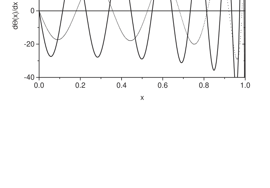
Figure 5: The function $d\Theta(x)/dx$ is plotted against $x$ with eigenvalue $b^{2}=119$ for $n=13$ in segmented line and $b^{2}=200$ for $n=23$ in solid line to show the structure of $B_{r}$ in space.

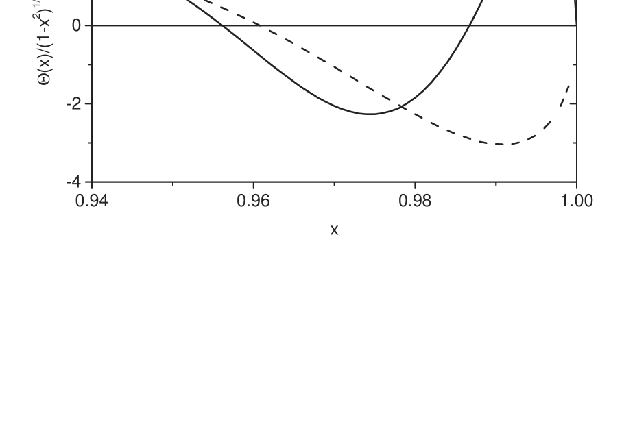
Figure 6: The function $\Theta(x)/(1-x^{2})^{1/2}$ is plotted against $0.94<x<1.0$ with eigenvalue $b^{2}=119$ for $n=13$ in segmented line and $b^{2}=200$ for $n=23$ in solid line to show the detail structure of $B_{\theta}$ and $B_{\phi}$ near the polar axis.

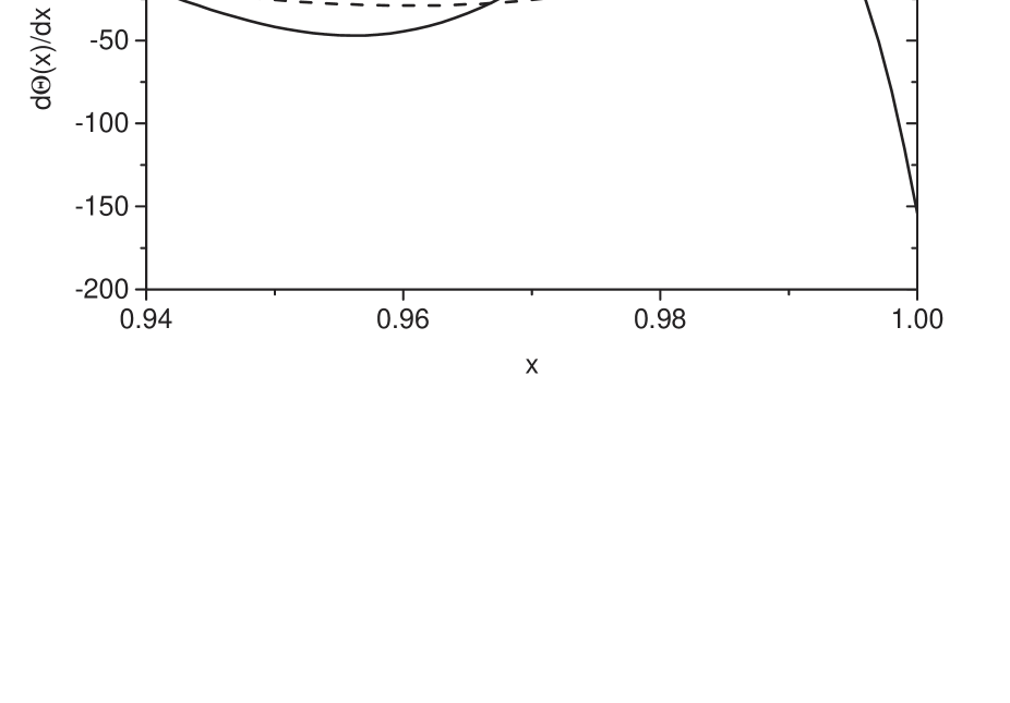
Figure 7: The function $d\Theta(x)/dx$ is plotted against $0.94<x<1.0$ with eigenvalue $b^{2}=119$ for $n=13$ in segmented line and $b^{2}=200$ for $n=23$ in solid line to show the detail structure of $B_{r}$ near the polar axis.

To consider the collimation of polar jets, we examine the magnetic field components. For $B_{\theta}$ and $B_{\phi}$ components, we plot the function $\Theta(x)/(1-x^{2})^{1/2}$ in Fig.(4) with the corresponding eigenvalue $b^{2}=119$ for $n=13$ according to Fig.(2). It peaks up off the scale to (-3.0) as $x$ approaches unity, but plunges to null at $x=+1$. As $n$ increases, the peak edges closer to $x=+1$. This is clearly shown in Fig.(4) with $b^{2}=200$ for $n=23$. The peak then goes to (+3.8) in this case. As a consequence, the peak rises up in amplitude but narrows down in width. To examine $B_{r}$, we plot the function $d\Theta(x)/dx$ in Fig.(5) which shows that the magnetic field is purely radial on the polar axis. As we have said, this radial magnetic field changes sign as each region of $\eta_{i}$ is crossed. With $n=13$ and $n=23$, the peak on the polar axis is (+71) and (-155) respectively. The magnetic energy is the quadratic quantity of this, and it peaks even more with respect to the off axis lobes. The detail structures near the polar axis are shown in Fig.(6) for $B_{\theta}$ and $B_{\phi}$, and in Fig.(7) for $B_{r}$. The magnetic field, therefore, converges to the polar axis as $n$ increases leading to a jet structure. Comparing the equatorial lobe of the magnetic field with the polar lobe, it is clear that the polar lobe is much narrower than the equatorial one. This lobe pattern is similar to directional antenna arrays. Due to the oscillating nature of Eq.(19a), there are spherical toroids, or secondary plasmoids, formed by closed magnetic field lines along this narrow peak. The number of secondary plasmoids embedded in this peak measures the number of zeros of Eq.(19a) contained within $a\eta_{0}$. The magnitude of $a\eta_{0}$ also indicates the large amplitude of $B_{\phi}$ through $\bar{Q}=a\bar{P}$ of Eq.(18a) which is itself consistent to the magnetic field convergence onto the polar axis.

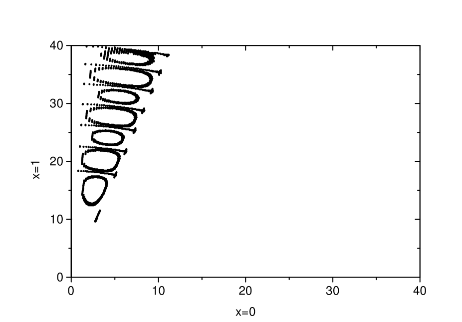
Figure 8: The field lines on the $(r-\theta)$ cone around the polar axis are plotted with $a\eta_{0}=40$ and a not so large $n=13$ for better resolution. The regions are divided by $C=0$ with plasmoids having $C=-0.010$ and $C=+0.005$.

To understand the magnetic structure of the jet, we plot the contours of $\bar{P}$ given by Eq.(20b) which amount to closed field lines of embedded secondary plasmoids. A contour plot in Fig.(8), similar to Fig.(1) but with $n=13$ and $b^{2}=119$, shows plasmoids along the polar cone that goes from $x=0.96$ to $x=1$, as in Fig.(7), which corresponds to a cone angle of about 14 degrees. The radial label goes from $a\eta=0$ to $a\eta=40$, and this interval is divided into seven regions set by the zeros of the spherical Bessel function. The first zero is at $a\eta=18.40$ and the subsequent zeros are approximately equally spaced, as indicated in Fig.(8). Negative contours of $C=-0.010$ are plotted in the first, third, fifth, and seventh regions only. Likewise, positive contours of $C=+0.005$ are plotted in second, fourth, and sixth regions. To avoid over crowdedness, the $C=-0.005$ contours are not plotted in the odd numbered regions, and the $C=+0.010$ ones are not shown in the even numbered regions. Once more, we recall that the magnetic field lines of these secondary plasmoids circle in alternating sequence. The boundary of the jet is given by the root of $\Theta(x)$ with $x_{j}=0.96$. At this boundary, the magnetic field is purely radial but alternates in sign. The other boundary is at $x_{j}=1.0$ where the magnetic field is also radial and alternates in sign opposite to that of $x_{j}=0.96$. Together with the roots of $R(\eta)$ at $\eta_{i}$ where the magnetic field is meridian, the plasmoids are magnetic vortices bounded by closed field lines at the border of each region. By axisymmetry, these poloidal magnetic contours rotate about the polar axis to generate tightly wounded toroids. Furthermore by axisymmetry, the toroidal azimuthal field lines are decoupled from the bipolar poloidal field lines. The field lines are, therefore, two-dimensional. As in the discussions concerning Fig.(1), this amounts to the $m=0$ mode in the Fourier transform $e^{im\phi}$ of the toroidal dependence.

The magnetic structure of this spherical temporal self-similar model, which shows a sequence of magnetic toroids along the jet, differs from the continuous helical field line structure in the cylindrical spatial self-similar model, complemented by numerical simulations [Casse 2004]. To understand the differences, the spatial cylindrical model has an imposed initial magnetic configuration everywhere in space. Jets are formed by transporting the disk plasma from the disk plane to the axis through magnetocentrifugal action. They are maintained along the axis by bringing disk plasma continuously in steady state to overcome transport losses. In this description, spatially self-similar jets in $z/r$ were formed in their present position in the distant past, and are maintained there continuously at the present and in the future.

As for the temporal self-similar spherical model, the disk plasma is first accreted to the galactic nucleus which builds up the plasma pressure there. While the plasma is in this bounded region, self-organization is nourished through dissipations to self-similar structures in $\eta=r(t)/y(t)$ calculated here, including the jets. The force-free configuration and the vortex nature of the magnetic field are akin to the quadratic quantities of magnetic helicity and cross helicity of the ideal MHD system. We note that $\eta$ is time invariant, such that the temporal self-similar $\eta$ profiles in magnetic field and plasma parameters maintain their forms at the very beginning. Later on, the self-similar MHD plasma errupts from the center outward, and this entire structure expands into the previously void space as time progresses, and continues to do so until the plasma density and magnetic field intensity get so low that they fade into space light years away. The bounded state and the erruption are described by the time evolution function $y(t)$, and it will be solved consistently in the next section.

7 Evolution Function

The $r$ component of the momentum equation reads

$$\rho[{\partial v\over\partial t}+v{\partial v\over\partial r}]+{d\over dr}p(r,P(r,\theta))+\rho{GM\over r^{2}}\,$$

$$=\,-{1\over\mu}({1\over r\sin\theta})^{2}{\partial P\over\partial r}\{{\partial^{2}P\over\partial r^{2}}+{1\over r^{2}}\sin\theta{\partial\over\partial\theta}({1\over\sin\theta}{\partial P\over\partial\theta})+Q{\partial Q\over\partial P}\}\,\,\,.$$

The term $dp/dr$ on the left side refers to radial derivatives for the explicit dependence and the implicit dependence in $P$. Making use of the $\theta$ component, Eq.(15a), the equation above becomes

$$\rho[{\partial v\over\partial t}+v{\partial v\over\partial r}]+{d\over dr}p(r,P(r,\theta))+\rho{GM\over r^{2}}\,$$

$$=\,-{1\over\mu}({1\over r\sin\theta})^{2}{\partial P\over\partial r}\{-\mu r^{2}\sin^{2}\theta{\partial p\over\partial P}\}\,=\,+{\partial P\over\partial r}{\partial p\over\partial P}\,\,\,.$$

The right side is just the radial derivative of plasma pressure on the implicit dependence in $P$. This cancels the corresponding term on the left side leaving only the explicit radial derivative

$$\rho[{\partial v\over\partial t}+v{\partial v\over\partial r}]+{\partial p(r,P)\over\partial r}+\rho{GM\over r^{2}}\,=\,0\,\,\,.$$

In terms of self-similar parameters, this equation reads

$$y^{2}{d^{2}y\over dt^{2}}+{1\over\eta}\{y^{4-3\gamma}{1\over\bar{\rho}}{\partial\bar{p}\over\partial\eta}+{GM\over\eta^{2}}\}\,=\,y^{2}{d^{2}y\over dt^{2}}+{1\over\eta}\{{1\over\bar{\rho}}{\partial\bar{p}\over\partial\eta}+{GM\over\eta^{2}}\}\,=\,0\,\,\,.$$

With $\alpha$ as the separation constant, and $H$ as an integration constant, the evolution function is, therefore, described by

$$y^{2}{d^{2}y\over dt^{2}}\,=\,+\alpha\,\,\,,$$

$$[{1\over 2}({dy\over dt})^{2}+{\alpha\over y}]\,=\,H\,\,\,,$$

$${dy\over dt}\,=\,\pm[2(H-{\alpha\over y})]^{1/2}\,\,\,.$$

To understand the meaning of $\alpha$, we note that plasma acceleration in Lagrangian coordinate is

$${dv\over dt}\,=\,\eta{d^{2}y\over dt^{2}}\,=\,{\alpha\eta\over y^{2}}\,=\,{\alpha\eta^{3}\over r^{2}}\,\,\,.$$

A negative $\alpha$ means an outward decelerating flow, or an inward accelerating flow. The deceleration gets smaller as $y$ or as $r$ gets larger, the acceleration gets larger as $y$ or as $r$ gets smaller. As for the meaning of $H$, we take the limit $y=\infty$ which gives $H/4\pi=(v^{2}/2)/4\pi\eta^{2}$ by using $r=\eta y$. Physically, this is the asymptotic radial kinetic energy per unit mass per unit area of a Lagrangian fluid element. For circular orbits, we would have $H=0$. Furthermore, we can rewrite Eq.(23a) making use the above physical expression of $\alpha$ to get

$$\rho\eta^{2}H\,=\,{1\over 2}\rho v^{2}+(\hat{r}\cdot\vec{F})r\,\,\,,$$

where $\vec{F}$ denotes all the forces on the right side of Eq.(2). It is clear that $H$ measures the total energy of the fluid element.

To consider the accretion disk magnetospheric plasma, we take $\alpha=-|\alpha|<0$ negative for an inward axcelerating flow. With $H=0$ as the boundary condition at infinity, we get

$${dy\over dt}\,=\,\pm({2|\alpha|\over y})^{1/2}\,=\,-({2|\alpha|\over y})^{1/2}\,\,\,.$$

The two signs for the square root correspond to the outward and inward flows. Taking the negative sign for the inward flow, the equatorial accretion disk plasma starts at infinity with an asymptotically zero radial velocity and ends near the center with a large influx.

As to describe the polar jets, we again take $\alpha=-|\alpha|<0$ negative. We consider $H=\pm|H|$ which lead to

$${dy\over dt}\,=\,\pm[2(\pm|H|+{|\alpha|\over y})]^{1/2}\,\,\,.$$

For $H=+|H|>0$ and taking the positive sign on the square root, this gives a decelerated outward flow. The deceleration gets smaller as $y$ or as $r$ gets larger, with the terminal velocity given by $v=\eta dy/dt=\eta(2H)^{1/2}$. For $H=-|H|<0$, the outward flow would stop at $y=|\alpha|/|H|$ where $dy/dt=0$. This $H=-|H|<0$ outward flow would be followed by an accelerated inward flow, should we take the negative sign on the square root, so that the system would be periodic and bounded. We, therefore, see that the system would make a transition from a bounded to an unbounded state when $H$ goes from negative to positive. The bounded state allows us to define the boundaries of the radial label $(0,\eta_{0})$ such that $(0<\eta<\eta_{0})$. The solutions of the evolution function in Eq.(24b) suggest that jets are a result of an erruptive process. This process is fed by plasma accretion from the galactic disk. As pressure builds up at the center, the plasma begins to oscillate, or to pulse, as described by the bounded solution with $H=-|H|<0$. We believe that it is during this phase that self-organized and self-similar structures in plasma parameters and magnetic fields would be nourished through dissipations. The dynamics is given by self-similar solutions where the magnetic fields are self-consistent to the plasma pressure that plays the role of the eigenvalue. The jet structure emerges along the polar axis as the eigenfunction of the magnetic field. By further pressure built-up and energy influx, $H=+|H|>0$ becomes positive, and the structure eventually errupts.

8 Rayleigh-Benard Cells

Now we have presented the general structure of galactic jets. It begins with an influx of plasmas from the accretion disk which drives up the plasma pressure at the galactic nucleus. The MHD plasma responses to self-organization by oscillating, or pulsating, periodically in time. As $H$ goes from negative to positive, the periodic mode goes to an erruptive mode. The result of self-organization is a structured configuration in space. This structure is not unique. For galactic jets, we have solved the system with the method of separation of variables as such that it ressembles to observations. This structure contains basically convective cells in space where magnetic field lines in adjacent cells rotate in opposite sense. Although such a structured configuration with consistent evolution function is in accordance with the time-dependent MHD equations, there is no mention of the initial configuration that could lead to such self-similar states. Consequently, such a highly organized complex structure could be regarded as an artificial result due to special mathematical constructions, which might not have any relevance to the physical jet system. In order to bring more reality to this analytic result, we recall the classical case of Rayleigh-Benard fluid self-organization. Consider a thin layer of oil heated from below, observations tell us that this simple homogeneous configuration will develope an array of identical hexagonal convective cells if the temperature gradient across the layer is sufficiently large. The velocity streamlines of adjacent cells rotate in opposite sense. Should the initial state of this oil layer be altered by arbitrary fluctuations, same convective cells would still appear after the initial fluctuations are dissipated. Numerically, such self-organized complex structure could be reached from the simple homogeneous initial configuration if the code is adequately pushed in the correct direction.

Guided by this fluid example, the self-similar jet structure could be regarded as the Rayleigh-Bernard equivalent in the MHD system. We could choose an initial state by taking $n=1$ in our solutions with plasma bounded between an outer sphere $\eta_{0}$ and an inner sphere $\eta_{*}$. This would give a large global long wavelength structure in the spherical layer. We consider an equilibrium state with $\alpha=-|\alpha|<0$ and $H=-|H|<0$ with $y=|\alpha|/|H|$ and $dy/dt=0$. Let us take this moment as $t=0$. An energy source in terms of pressure is supplied by the accretion disk to pump the MHD plasma at the lower boundary $\eta_{*}$. At some moment, $y$ begins to depart from its equilibrium to fall towards the center due to perturbations. Like in the oil layer case, this could trigger convections so that the long wavelength global structure cascades to short wavelength structures accepted by the system. Cenvective cell scaling becomes smaller as $n$ gets larger. Different from the flat layer fluid case, the convective cells in this spherical MHD layer are not identical, since there is a focusing effect to the polar axis.

9 Mass Density Profile

As for the spatial part, we have

$${1\over\bar{\rho}}{\partial\bar{p}\over\partial\eta}+{GM\over\eta^{2}}\,=\,-\alpha\eta\,\,\,.$$

With $\bar{p}$ given by Eq.(18b), the above equation gives

$$\bar{\rho}(\eta,\bar{P})\,=\,(\eta^{-3})({4\bar{p}_{2}(\bar{P})\over\alpha\eta^{3}+GM})\,=\,(\eta^{-3})({4\bar{p}_{2}(\bar{P})\over GM})\,$$

$$=\,(\eta^{-3})({4\over GM})(b^{\prime 2}\bar{P}^{2}+\bar{C})\,=\,\bar{\rho}_{1}(\eta)\bar{\rho}_{2}(\bar{P})\,\,\,.$$

In our present case, we are considering a spherical shell domain that the radial label $\eta=0$ is excluded. The negative powers of $\eta$ in plasma pressure and mass density do not cause singularity. We have set $\alpha=0$, with vanishing net force on the flow, to obtain the second equality in Eq.(25) to be compatible with the functional form of $F=F(P)$ with $\gamma=4/3$. Nevertheless, we could relax this condition to $\alpha\approx 0$ such that $\alpha\eta^{3}<<GM$. To understand the implication of such inequality, we remark that

$${\alpha\eta^{3}\over GM}\,=\,{dv/dt\over GM/r^{2}}\,<<\,1\,\,\,.$$

Therefore, it is just the acceleration of the flow to that of the central mass gravitational acceleration. Since $dv/dt$ gets smaller as $r$ gets larger with $1/r^{2}$ scaling, this condition establishes that self-similar configurations can be organized, and bounded oscillations of the $H=-|H|<0$ case can take place, as long as the plasma acceleration is much less that the gravitational acceleration. To close the entire self-similar system, we now come to the functional $F(P)$ for the adiabatic equation of state. With the results in Eq.(18b) and Eq.(25) using $\alpha\approx 0$, we have

$$\bar{F}(\bar{P})\,=\,{\bar{p}_{2}(\bar{P})\over\bar{\rho}_{2}^{\gamma}(\bar{P})}\,=\,({GM\over 4})^{4/3}\bar{p}_{2}^{-1/3}(\bar{P})\,=\,({GM\over 4})^{4/3}(b^{\prime 2}\bar{P}^{2}+\bar{C})^{-1/3}\,\,\,.$$

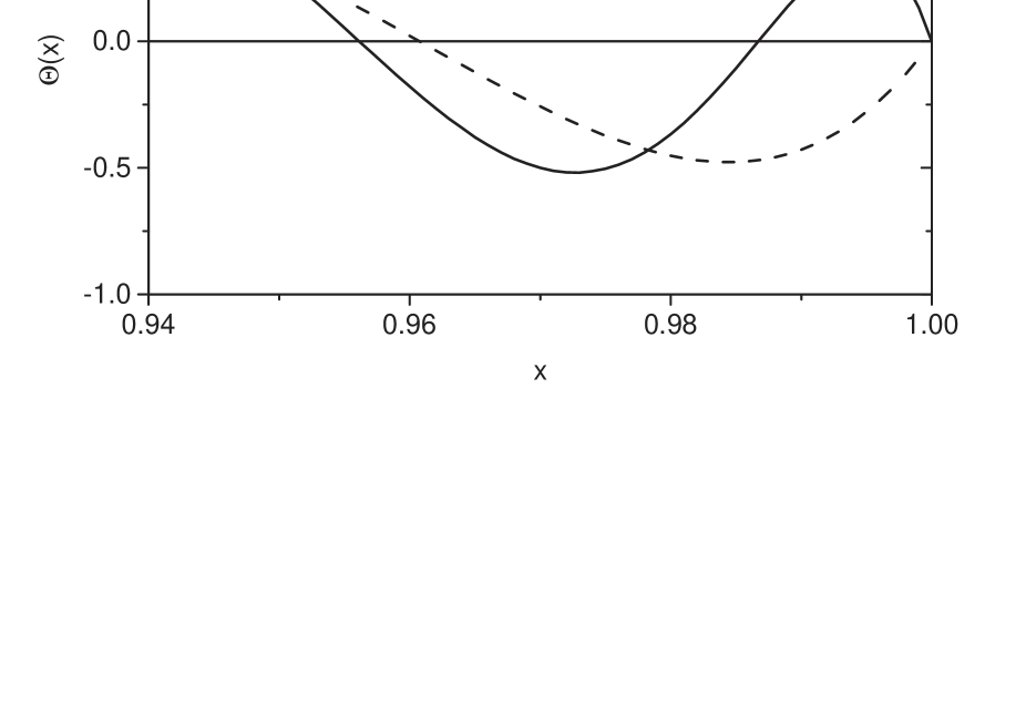
Figure 9: The eigenfunction $\Theta(x)$ is plotted against $0.94<x<1.0$ with eigenvalue $b^{2}=119$ for $n=13$ in segmented line and $b^{2}=200$ for $n=23$ in solid line to show its dependence on $n$.

To understand the plasma structure of the jet, we note that the plasma pressure and mass density are $b^{\prime 2}\bar{P}^{2}(\eta,x)+\bar{C}$ dependent which means positive definite $b^{\prime 2}C^{2}+\bar{C}$ dependent, according to Eq.(18b) and Eq.(25) respectively. The plasma pressure and the mass density have their minimum at $\bar{P}(\eta,x)=(a\eta)^{1/2}J_{n+1/2}(a\eta)\Theta(x)=0$. This minimum is positive nonzero because of the positive integration constant $\bar{C}$ in Eq.(18b). To discuss the plasma structure in the jets, we reproduce the part of Fig.(3) in the range $0.94<x<1.0$ in Fig.(9). The segmented line for $n=13$ has $\Theta(x)=0$ at the cone boundary $x=0.96$ and at the cone center $x=1.0$. In between, there is a minimum at $x=0.985$. Because of the quadratic dependence $\Theta^{2}(x)$, these features correspond to a cavity-like structure for the plasma pressure and mass density of the jet, compatible to numerical simulations of the time-dependent dissipative MHD equations [Casse 2004, Zanni et. al. 2004]. Other than the zeros of $\Theta(x)$, $\bar{P}(\eta,x)$ also vanishes at radial locations where $J_{n+1/2}(a\eta)=0$. With the quadratic dependence

$$R^{2}(\eta)\,=\,(a\eta)J^{2}_{n+1/2}(a\eta)\,\,\,,$$

there are ripples for plasma pressure and mass density along the radial label. The radial function has two contributions. The part of the Bessel function $J_{n+1/2}(a\eta)$ has an oscillating nature with decreasing amplitude, while the part of $(a\eta)$ has an increasing amplitude that helps to maintain the ripple level of $R^{2}(\eta)$. The peaks of these ripples are at the topological center of each plasmoid which is the magnetic axis of the toroid where $B_{\phi}$ has a maximum line integral. These ripples are also seen in numerical simulations [Zanni et. al. 2004]. It is quite surprising that the results of this spherical temporal self-similar MHD model agree rather well qualitatively with numerical simulations of the time-dependent MHD equations for the cylindrical magnetocentrifugaling model. Both of them give cavity structures in the transverse direction and ripple structures in the longitudinal direction.

The polar jets, therefore, have a periodic and approximately equally spaced concentration of plasmoids in its longitudinal direction, except the first region which is more extensive. The closed magnetic field lines for adjacent plasmoids rotate in opposite sense. The plasma pressure and mass density have a hollow conic structure with ripples along the radial direction. Such periodic structure happens to be compatible with radio observations where high intensity islands are mapped. These islands are usually thought to be periodic ejections of mass from the accretion disk. According to our model, they are rather the internal spatial arrangments of an expanding jet driven by an erruptive event.

10 Discussions and Conclusions

One of the main objections of self-organized plasmoid representation in free space in the absence of an adequate boundary is that it apparently violates the Virial theorem which states that [Schmidt 1966]

$${1\over 2}{d^{2}I\over dt^{2}}+\int x_{k}{\partial G_{k}\over\partial t}dV\,=\,2(T+U)+W^{E}+W^{M}-\int x_{k}(P_{ik}+T_{ik})dS\,\,\,,$$

where $I$ is the moment of inertia of the plasmoid, $G$ is the momentum density of the electromagnetic field, $T$ and $U$ are the kinetic and thermal energies of the plasma, $W^{E}$ and $W^{M}$ are the electric and magnetic energies in the volume, $P_{ik}$ and $T_{ik}$ are the plasma and electromagnetic stress tensors. Taking the volume to cover the entire plasma and field, the surface term on the right side vanishes. In laboratory plasmas, this surface could be the machine vessel. Should the plasmoid be stationary, the volume term on the left side would be null, and the moment of inertia would be accelerating since the terms on the right side are all positive definite. While this statement has no conflict with the unbounded solutions, it apparently contradicts the stationary state of the bounded solutions. Nevertheless, this argument has overlooked the asymptotically bounded nature of the $H=-|H|<0$ plasmoid state. In this asymptotic case, we have $dI/dt=(dI/dy)(dy/dt)=0$ so that $I$ is stationary. The fact that $d^{2}I/dt^{2}>0$ implies that $I$ is at an asymptotic minimum, not an acceleration of $I$, which complies with the Virial theorem.

The classical accretion-ejection model of Blandford and Payne [1982] is a time-independent stationary state model with spatial self-similar MHD solutions in cylindrical geometry $(r,\phi,z)$ with Alfvénic plasma flow velocity plus a rotation, all with Keplerian scaling. In this model, the jets are formed by convecting the magnetospheric disk plasmas from the disk plane to the axis by magnetocentrifugal action through the magnetic field lines with low inclination angles to the disk plane. The angular momentum of the plasma on the disk plane is focused to the axis. The jets were put in place in the distant past according to the spatial self-similar solutions in $z/r$, and are maintained there by continuously transporting disk plasmas to the axis to sustain the axial outflow. Collimation to the axis is accomplished by magnetic hoop force.

Here, we have taken a dynamic view where jets are the consequences of erruptive events, based on time-dependent MHD equations in spherical geometry $(r,\theta,\phi)$. The disk plasmas are accreted to the galactic nucleus where plasma pressure is built up to cause an erruption. The radially symmetric expanding velocity interacts the plasma with the magnetic field self-consistently through the MHD equations to generate spatial structures. Due to the existence of multiple quadratic invariants in the absence of dissipations, MHD systems have the tendency of developing self-organized and self-similar states through dissipative processes. The force-free configuration and the vortex nature of the magnetic field are akin to the quadratic invariants of the magnetic helicity and cross helicity of the MHD system. For these reasons, although temporally self-similar solutions are only a subset of general time-dependent MHD solutions, these self-similar configurations are prone to develope in natural phenomena.

We, therefore, describe these spatial structures by self-similar temporal solutions in $\eta=r/y$. In this self-similar spherical model, consistent self-similar representations of plasma pressure, mass density, and magnetic fields are worked out for the $\gamma=4/3$ BC Low model, with special emphasis on the finite $\beta$ case. The spatial distribution of the magnetic field is described by an equation where the plasma pressure acts as the eigenvalue. The nature of this eigenvalue equation is as such that the magnetic field gets converged to the polar axis as a response to the high plasma pressure directly related to the eigenvalue. Since the separation constant $n(n+1)$ in this eigenvalue equation is a free parameter that as yet to be specified, there will be an adequate $n$ for almost any given plasma pressure. Although the radial plasma velocity is isotropic, the spatial structures are not. They could be highly collimated along the axial direction, and expand into the previously void space as time progresses.

Although other types of solutions are permitted, we have specifically examined the solutions that bear resemblance with jet features with $n\gg 1$ and $a\eta_{0}\gg 1$. Since plasma and magnetic field are frozen into each other, plasma outflow is also collimated to the polar axis. The existence of regions of closed field lines along the primary polar magnetic lobe permits secondary plasmoids be embedded in it. These secondary plasmoids appear to be compatible to the observed islands of radio intensities. The time evolution function of the radial velocity consistent to the temporal self-similar solutions has different types of solutions according to the sign of $H$. Although the equatorial disk magnetospheric plasma is not addressed here, the accelerated accretion of plasma influx could be modelled with $H=0$ as the boundary condition at infinity. As for the polar jets, $H<0$ gives a bounded oscillating, or pulsating, solution. This bounded stage, we believe, nourishes the self-organized and self-similar states. With $H>0$, it gives an unbounded expanding solution with a high terminal velocity. It is apparent that plasma pressure due to accretion is the prime driving force that determines the value of $H$. The bounded oscillation would make a transition to the unbounded expansion as $H$ goes from negative to positive. According to our model, jet structures are, therefore, considered as a spatial configuration that has been expanding continuously into space.

References

- (1) Aly, J.J., 1984. On Some Properties of Force-Free Magnetic Fields in Infinite Regions of Space, Astrophysical Journal 283, 349-362.
- (2) Balbus, S.A. and Hawley, J.F., 1998. Instability, turbulence, and Enhanced Transport in Accretion Disks, Review of Modern Physics 70, 1-53.
- (3) Blandford, R.D. and Payne, D.G., 1982. Hydromagnetic Flows from Accretion Discs and the Production of Radio Jets, Monthly Notices of the Royal Astronomical Society 199, 883-903.
- (4) Cao, X. and Spruit, H.C., 1994. Magnetically Driven Wind from an Accretion Disk with Low-Inclination Field Lines, Astronomy and Astrophysics 287, 80-86.
- (5) Casse, F. and Ferreira, J., 2000a. Magnetized Accretion-Ejection Structures, IV. Magnetically-Driven Jets from Resistive, Viscous, Keplerian Discs, Astronomy and Astrophysics 353, 1115-1128.
- (6) Casse, F. and Ferreira, J., 2000b. Magnetized Accretion-Ejection Structures, V. Effects of Entropy Generation Inside the Disc, Astronomy and Astrophysics 361, 1178-1190.
- (7) Casse, F., 2004. MHD Accretion-Ejection Flows, Astrophysics and Space Science 293, 91-98.
- (8) Contopoulos, J., 1995. A Simple Type of Magnetically Driven Jets: an Astrophysical Plasma Gun, Astrophysical Journal 450, 616-627.
- (9) Contopoulos, J. and Lovelace, R.V.P., 1994. Magnetically Driven Jets and Winds: Exact Solutions, Astrophysical Journal 429, 139-152.
- (10) Ferreira, J. and Pelletier, G., 1995. Magnetized Accretion-Ejection Structures, III. Stellar and Extragalactic Jets as Weakly Dissipative Disk Outflows, Astronomy and Astrophysics 295, 807-822.
- (11) Gibson, S.E. and Low, B.C., 1998. A Time-Dependent Three-Dimensional Magnetohydrodynamic Model of the Coronal Mass Ejection, Astrophysical Journal 493, 460-473.
- (12) Hasegawa, A., 1985. Self-Organization Processes in Continuous Media, Advances in Physics 34, 1-42.
- (13) Kato, S., Kudoh, T., and Shibata, K., 2002. 2.5 Dimension Nonsteady Magnetohydrodynamic Simulations of Magnetically Driven Jets from Geometrically Thin Disks, Astrophysical Journal 565, 1035-1049.
- (14) Keppens, R., Casse, F., and Goedbloed, J.P., 2002. Waves and Instabilities in Accretion Disks: Magnetohydrodynamic Spectroscopic Analysis, Astrophysical Journal 569, L121-L126.
- (15) Krasnopolski, R., Li, Z.Y., and Blandford, R.D., 1999. Magnetocentrifugal Launching of Jets from Accretion Disks. I. Cold Axisymmetric Flows, Astrophysical Journal 526, 631-642.
- (16) Livio, M., 1997. IAU Colloquium 163. ASP Conference Series, Vol. 121, p. 845, eds. D.T. Wickramasinghe, G.V. Bicknell, L. Ferrario.
- (17) Low, B.C., 1982a. Self-Similar Magnetohydrodinamics. I. The Polytrope and the Coronal Transient, Astrophysical Journal 254, 796-805.
- (18) Low, B.C., 1982b. Self-Similar Magnetohydrodinamics. II. The Expansion of a Stella Envelope into a Surrounding Vacuum, Astrophysical Journal 261, 351-369.
- (19) Low, B.C., 1984a. Self-Similar Magnetohydrodinamics. III. The Subset of Spherically Symmetric Gasdynamic Flows, Astrophysical Journal 281, 381-391.
- (20) Low, B.C., 1984b. Self-Similar Magnetohydrodinamics. IV. The Physics of Coronal Transients, Astrophysical Journal 281, 392-412.
- (21) Low, B.C., 1986. Blowup of Force-Free Magnetic Fields in the Infinite Region of Space, Astrophysical Journal 307, 205-212.
- (22) Low, B.C. and Lou Y.Q., 1990. Modeling Solar Force-Free Magnetic Fields, Astrophysical Journal 352, 343-352.
- (23) Lynden-Bell, D. and Boily, C., 1994. Self-Similar Solutions up to Flashpoint in Highly Wound Magnetostatics, Monthly Notices of the Royal Astronomical Society 267, 146-152.
- (24) Matsumoto, R. et al, 1996. Radio Jets and the Formation of Active Galaxies: Accretion Avalanches on the Torus by the Effect of a Large-Scale Magnetic Field, Astrophysical Journal 461, 115-126.
- (25) Osherovich, V.A., Farrugia, C.J., and Burlaga, L.F., 1993. Nonlinear Evolution of Magnetic Flux Ropes. 1. Low-Beta Limit, Journal of Geophysical Research 98, 13225-13231.
- (26) Osherovich, V.A., Farrugia, C.J., and Burlaga, L.F., 1995. Nonlinear Evolution of Magnetic Flux Ropes. 2. Finite-Beta Plasma, Journal of Geophysical Research 100, 12307-12318.
- (27) Ouyed, R. and Pudritz, R., 1997. Numerical Simulations of Astrophysical Jets from Keplerian Disks. I. Stationary Models, Astrophysical Journal 482, 712-732.
- (28) Schmidt G., 1966. Physics of High Temperature Plasmas, Academic Press, New York, Chapter III.
- (29) Tsui, K.H., 2006. A Self-Similar Magnetohydrodynamic Model for Ball Lightnings, Physics of Plasmas 13, 072102.
- (30) Tsui, K.H., 2007. Self-Similar Magnetohydrodynamic Model of Magnetic Clouds, Journal of Atmospheric and Solar-Terrestrial Physics, to be published.
- (31) Tsui, K.H. and Tavares, M.D., 2005. Self-Similar Evolution of the Two-Dimensional Cylindrical Magnetohydrodynamic Flux Rope, Journal of Atmospheric and Solar-Terrestrial Physics 67, 1691-1696.
- (32) Ustyugova, G.V., Koldoba, A.V., Romanova, M.N., Chetchetkin, V.M., and Lovelace, R.V.E., 1995. Magnetohydrodynamic Simulations of Outflows from Accretion Disks, Astrophysical Journal 439, L39-L42.
- (33) Vlahakis, N., 2004. The efficiency of the Magnetic Acceleration in Relativistic Jets, Astrophysics and Space Science 293, 67-74.
- (34) Zanni, C., Ferrari, A., Massaglia, S., Bodo, G., and Rossi, P., 2004. On the MHD Acceleration of Astrophysical Jets, Astrophysics and Space Science 293, 99-106.