L1Packv2: A Mathematica package for minimizing an $\ell_{1}$-penalized functional

Abstract

L1Packv2 is a Mathematica package that contains a number of algorithms that can be used for the minimization of an $\ell_{1}$-penalized least squares functional. The algorithms can handle a mix of penalized and unpenalized variables. Several instructive examples are given. Also, an implementation that yields an exact output whenever exact data are given is provided.

1 Introduction

In physical and applied sciences, one often encounters the situation where the quantities in which one is ultimately interested cannot be measured directly. Such a situation appears e.g. in magnetic resonance imaging (Fourier components of an image are measured), optics (convolution of an object with a non-trivial point spread function forms an image) etc.

Often, it happens that a linear relationship exists between the data and the quantities of interest. Nonetheless, several issues stand in the way of ‘solving’ such linear inverse problems. Frequently, the data are incomplete (underdetermined system from a mathematical point of view) and contaminated with noise (inconsistent equations from a mathematical point of view). Moreover, the linear operator linking both is often singular.

A much-used strategy to arrive at a well-defined solution for the above mentioned linear equations, is to formulate the problem as the minimization of a quadratic functional consisting of the sum of the discrepancy $\|Kx-y\|^{2}$ and a penalization contribution $\|x\|^{2}$:

$$\arg\min_{x}\|Kx-y\|^{2}+\lambda\|x\|^{2}$$ (1)

in terms of the noisy data $y$ and the linear operator $K$. The regularization parameter $\lambda$ controls the trade-off between the data misfit $y-Kx$ and the $\ell_{2}$-norm of the model parameters. With a proper choice of $\lambda$, the influence of noise (present in the data $y$) on the reconstruction of $x$ can now be kept under control [1, 2, 3].

The resulting variational equations

$$K^{T}Kx+\lambda x=K^{T}y$$ (2)

for the minimization problem (1) are linear; a considerable advantage of this technique is that existing efficient linear solvers (i.e. thoroughly tested algorithms and computer software) can be used. A disadvantage of using a penalty term of type $\lambda\|x\|^{2}$ is that it is quite generic and does not take into account any a priori information that one may have about the desired reconstructed object (other than being of finite size).

Recently, scientist have become interested in using ‘sparsity-promoting’ penalizations for the solution of linear ill-posed inverse problems. In particular, the following minimization problem involving an $\ell_{1}$-penalized least squares functional has attracted a great deal of attention:

$$\bar{x}(\lambda)=\arg\min_{x}\|Kx-y\|^{2}+2\lambda\|x\|_{1}$$ (3)

for a given real matrix $K$, real data $y$ and positive penalization parameter $\lambda\geq 0$. The $\ell_{1}$-norm is defined as $\|x\|_{1}=\sum_{i}|x_{i}|$.

The minimization problem (3) is commonly referred to as ‘lasso’ after [4], although earlier uses of this technique do exist [5]. In the context of signal decomposition, the term ‘basis pursuit denoising’ is often used [6].

Compressed sensing [7, 8], a rapidly developing research area, is based on the realization that a signal of length $N$ can often be fully recovered by far fewer than $N$ measurements if it is known in advance that the signal is sparse. The recovery is done by calculating $\arg\min_{Kx=y}\|x\|_{1}$, or in case of the presence of noise by calculating the minimizer (3) for which it is known that $\bar{x}(\lambda)$ is typically sparse, i.e. a great number of its components are exactly zero (at least for a large enough penalty $\lambda$).

Unfortunately, the variational equations that describe the minimizer (3) are nonlinear (see equations (7) below). The use of a traditional $\ell_{2}$ penalization leads to linear equations but a non-sparse minimizer. Hence the question of finding ways of efficiently recovering the minimizer of functional (3) has attracted a great deal of interest [9, 10, 11, 12, 13].

The Mathematica package L1Packv2 implements a couple of algorithms for finding the minimizer (3). There are five iterative algorithms which yield an approximation of $\bar{x}(\lambda)$ when stopped after a finite number of steps. The principal algorithm however can calculate the minimizer $\bar{x}(\lambda)$ exactly (up to computer round-off) in a finite number of steps. This algorithm is known as the ‘homotopy method’ [14] or as Least Angle Regression (LARS) [15].

The algorithms in this package can also treat the minimization of a slightly more general functional:

$$\min_{x}\|Kx-y\|^{2}+2\lambda\sum_{i}w_{i}|x_{i}|$$ (4)

with positive (or zero) weights $w_{i}\geq 0$.

The procedures are all written with real matrices and signals in mind. They do not work for complex variables. Extension to complex data would require optimization over quadratic cones; the thresholded Landweber algorithm could be easily adapted, but not the other algorithms. The package was developed and tested with Mathematica 5.2 [16]. Other toolboxes geared towards the recovery of sparse solutions of linear equations exist for Matlab: SparseLab [17], $\ell_{1}$-magic [18].

2 Implementation

In order to describe the solution of the minimization problem (3), it is worthwhile mentioning the following four equivalent problems:

1. the minimization of the penalized least squares functional:

   $$\bar{x}(\lambda)=\arg\min_{x}\|Kx-y\|^{2}+2\lambda\|x\|_{1}$$ (5)

2. the constrained minimization problem:

   $$\tilde{x}(R)=\arg\min_{\|x\|_{1}\leq R}\|Kx-y\|^{2}$$ (6)

   (with an implicit relation between $R$ and $\lambda$, see below)

3. the solution of the variational equations:

   $$\begin{array}[]{lclcl}(K^{T}(y-K\bar{x}))_{i}&=&\lambda\;\mathrm{sign}(\bar{x}_{i})&\qquad\mathrm{if}&\bar{x}_{i}\neq 0\\ |(K^{T}(y-K\bar{x}))_{i}|&\leq&\lambda&\qquad\mathrm{if}&\bar{x}_{i}=0\end{array}$$ (7)

4. the solution of the fixed-point equation:

   $$\bar{x}=S_{\lambda}[\bar{x}+K^{T}(y-K\bar{x})],$$ (8)

   where $S_{\lambda}$ is soft-thresholding applied component-wise (see expression (13)).

One has $R=\|\bar{x}(\lambda)\|_{1}$ and also:

$$\lambda=\|K^{T}(y-K\bar{x}(\lambda))\|_{\infty}=\max_{i}|(K^{T}(y-K\bar{x}(\lambda)))_{i}|$$ (9)

which follows immediately from relations (7).

The equivalence of the four formulations (5–8) can easily be seen as follows: Constrained minimization (6) is turned into problem (5) by the introduction of a Lagrange multiplier $\lambda$. The variational equations (7) are derived from (5) by putting $x=\bar{x}+he_{i}$ (where $h$ is a small parameter and $e_{i}$ is the $i$th basis vector) and expressing that $\|K\bar{x}-y\|^{2}+2\lambda\|\bar{x}\|_{1}\leq\|Kx-y\|^{2}+2\lambda\|x\|_{1}$ for all $h$. The fixed-point equation (8) is derived from equation (7) by adding $x_{i}$ to both sides of the equalities, by rearranging terms and using $S_{\lambda}(u)=u-\lambda\,\mathrm{sgn}(u)$ for $|u|\geq\lambda$ and $S_{\lambda}(u)=0$ for $|u|\leq\lambda$.

It can be shown that $\bar{x}(\lambda)$ is a piecewise linear function of $\lambda$ and that $\bar{x}(\lambda)=0$ for $\lambda\geq\lambda_{\mathrm{max}}\equiv\max_{i}|(K^{T}y)_{i}|$. Hence, it is sufficient to calculate the nodes of $\bar{x}(\lambda)$; for generic values of $\lambda$ in between these nodes, one can use simple linear interpolation to determine $\bar{x}(\lambda)$.

The nodes of $\bar{x}(\lambda)$ can be calculated using only a finite number of elementary operations (addition, multiplication, …) using the LARS/homotopy method [14, 15]. In other words, despite the variational equations being nonlinear, they can still be solved exactly! In fact, the variational equations (7) are piece-wise linear and can be solved by starting from $\bar{x}(\lambda=\lambda_{\mathrm{max}})=0$ and letting $\lambda$ decrease: at each stage where a component of $\bar{x}(\lambda)$ becomes nonzero (or, in some exceptional cases, where it becomes zero again) a ‘small’ linear system has to be solved to ensure relations (7); this procedure is stopped when the desired value of $\lambda$ is reached (or when some other stopping criterium such as e.g. $\|\bar{x}\|_{1}=R$ or $|\mathrm{supp}\,(\bar{x})|=N$, … is satisfied).

Thus, the computational burden of such an algorithm consists of two contributions at every node: calculation of the remainder $K^{T}(y-Kx)$, and the solution of a linear system of size equal to the support size of that minimizer. The first contribution is the same at every step, the second is very small at the start (support size starts at 0) but dominates after a certain number of steps.

Such an algorithm is implemented in this Mathematica package under the name FindMinimizer. If $K$ and $y$ are given in terms of exact numbers (integer, rational, …), this algorithm will yield an exact answer. If approximate numbers are used as input, then the algorithm will output a numerical solution.

Other implementations exist (e.g. in Matlab [17, 19] or in R [15]), but they only work with approximate, floating-point, numbers. Being able to work with exact arithmetic is advantageous for pedagogical reasons: One can easily follow how the solution is found (the implementation can also print out intermediate results), at least for small matrices.

Another advantage of this implementation is that it is able to handle an exceptional case that is left unaddressed in [15, 17, 19]. Indeed, in [15] it is mentioned that their implementation of the algorithm cannot handle the case where two new indices may enter the support of $\bar{x}$ at the same time. Using floating-point data, this is indeed a rare occurrence, but using small integer matrices and data, it is easy to find such exceptions (see several fully worked-out examples in section 5). Section 5 describes how the present implementation deals with that case.

Probably the biggest advantage over existing software is that L1Packv2 can handle the problem of minimization of the functional

$$\bar{x}(\lambda)=\arg\min_{x}\|Kx-y\|^{2}+2\lambda\sum_{i}w_{i}|x_{i}|$$ (10)

with weights $w_{i}\geq 0$. If all weights are nonzero, then this can be reduced to the problem (5) by a simple rescaling of the independent variables. However, if zero weights are present, this is no longer true. Still, the implementation provided by L1Packv2 handles that case ([15, 17, 19] do not). The variational equations now are:

$$\begin{array}[]{lclcl}(K^{T}(y-K\bar{x}))_{i}&=&w_{i}\,\lambda\;\mathrm{sign}(\bar{x}_{i})&\qquad\mathrm{if}&\bar{x}_{i}\neq 0\\ |(K^{T}(y-K\bar{x}))_{i}|&\leq&w_{i}\,\lambda&\qquad\mathrm{if}&\bar{x}_{i}=0\end{array}$$ (11)

In case of the presence of unpenalized components ($w_{i}=0$ for some $i$), the biggest difference with the previous case is that the starting point is no longer the origin (and $\lambda_{\mathrm{max}}$ is no longer $\max_{i}|(K^{T}y)_{i}|$). Also, for a given minimizer $\bar{x}(\lambda)$, the penalty parameter equals

$$\lambda=\max_{i,w_{i}\neq 0}|(K^{T}(y-K\bar{x}))_{i}/w_{i}|$$ (12)

(compare with expression (9)). Other than that, the algorithm (broadly speaking) follows the same lines.

In addition to the LARS/homotopy method used in FindMinimizer, the package also provides five iterative algorithms for the minimization problems (5) and (6):

1. ThresholdedLandweber

2. ProjectedLandweber

3. ProjectedSteepestDescent

4. AdaptiveLandweber

5. AdaptiveSteepestDescent

After a finite number of steps, these yield an approximation of the minimizer. Whereas the LARS/homotopy method heavily is derived from the variational equations (7), the ‘thresholded Landweber’ method (see formula (15)) is inspired by the fixed-point equation (8). The formulation (6) lays at the basis of the remaining four algorithms 2–5, see formulas (16)–(19). They use projection on an $\ell_{1}$-ball, which can be calculated fairly easily in practice [10]. Two of these four algorithms use a path-following strategy (where the minimizer $\tilde{x}(R)$ is sought for a whole range $0\leq R\leq R_{\mathrm{max}}$, just as the LARS/homotopy method), whereas the other two only calculate the minimizer $\tilde{x}(R)$ for a specific value of $R$ (just as the ‘thresholded Landweber’ algorithm calculates $\bar{x}(\lambda)$ for a specific value of $\lambda$).

All algorithms have an option to generate a list of intermediate results at each step (i.e. each node for the exact method, and each iteration for the iterative methods). One can use the following variables: iterate or node number, time elapsed since start, $\bar{x}$, $y-K\bar{x}$, $K^{T}(y-K\bar{x})$ (without having to make additional matrix multiplications!) and any function of these. This is useful for evaluating the behavior of the algorithms, or e.g. for easily being able to plot the trade-off curve, $(\|\bar{x}(\lambda)\|_{1}$ vs. $\|K\bar{x}(\lambda)-y\|^{2})$ as a function of $\lambda$. An example is given in section 5.

3 Main algorithm

The main algorithm is called FindMinimizer and has syntax

FindMinimizer[K_, y_, options___].

It calculates the minimizer $\bar{x}(\lambda)$ of (3) with the ‘exact’ algorithm (i.e. homotopy method/LARS [14, 15]). It takes the operator $K$ and the data $y$ as input. The option Weights $\rightarrow w$ can be used to set the weights $w_{i}$ as in the formulation (10). The default for this option is all weights equal to $1$: $w_{i}=1$.

This algorithm starts from $\bar{x}=0$ (assuming no zero weights) and lets $\|\bar{x}\|_{1}$ grow, and $\lambda$ descend until a stopping condition is met. There are four different stopping criteria possible:

1. The option StoppingPenalty$\rightarrow\lambda$ will stop the algorithm when the penalty parameter reaches this value. In other words,

   FindMinimizer[$K$,$y$,StoppingPenalty$\rightarrow\lambda$]

   will calculate $\bar{x}(\lambda)$ as in (5). The default is StoppingPenalty$\rightarrow 0$.

2. The option MaximumL1Norm->$R$ will stop the algorithm when the $\ell_{1}$-norm of the minimizer reaches the value $R$. In other words, the command FindMinimizer[$K$,$y$,MaximumL1Norm$\rightarrow R$] will calculate $\tilde{x}(R)$ as in (6). The default is MaximumL1Norm$\rightarrow\infty$ which means that the default will never cause the algorithm to stop.

3. The option MinimumDiscrepancy->$d$ will make the algorithm stop when $\|K\bar{x}-y\|^{2}=d$. The default is MinimumDiscrepancy->0.

4. The option MaximumNonZero$\rightarrow N$ will stop at the first node of $\bar{x}$ having $N$ nonzero coefficients. The default is MaximumNonZero$\rightarrow\infty$. Unpenalized components ($i$ for which $w_{i}=0$) are always included in this count.

The use of StoppingPenalty, MinimumDiscrepancy or MaximumL1Norm allows the user to stop the algorithm at exactly that value of $\lambda$, $\|K\bar{x}-y\|^{2}$ or $\|\bar{x}(\lambda)\|_{1}$ respectively: the first node that overshoots this condition is computed, but linear interpolation with the previous node is used to arrive at exactly the value specified. This is very useful if you only need to find the minimizer $\bar{x}(\lambda)$ for one specific value of $\lambda$, $\|K\bar{x}-y\|^{2}$ or $\|\bar{x}\|_{1}$. There is no need to compile the list of intermediate nodes and no need for doing the interpolation manually.

Apart form the four specific stopping criteria above, one can also use a more general criterion: StoppingCondition$\rightarrow$cond. E.g. StoppingCondition:>(Time>=3) will make sure the algorithm stops at the first node that is calculated within 3 seconds. All the variables listed in table 1 can be used to express a stopping condition. The default is False meaning that it will not cause the algorithm to stop.

Notice that the default behavior will make the algorithm stop at the last node, for which $\lambda=0$ and $K^{T}(y-Kx)=0$. When using floating point data one should take care to specify a good stopping condition. Using floating point numbers, the default stopping condition, StoppingPenalty$\rightarrow 0$, most likely will not work (because $\max_{i}|(K^{T}(y-K\bar{x}))_{i}|$ will eventually be $\approx 10^{-16}$ or so, which is still strictly larger than $0$); In this case, it is best to specify an explicit stopping condition of type StoppingPenalty$\rightarrow\lambda$ with $\lambda>0$. One could also use MaximumL1Norm$\rightarrow R$ if one has a good idea for a suitable final $\|\bar{x}\|_{1}$.

The output of the FindMinimizer algorithm is of the form $\{\{\mathrm{collected\ data}\},\bar{x}\}$, or just $\bar{x}$ if no data are collected (default). The data that are to be collected at each node are described by the ListFunction option. Table 1 lists the variables that can be used. E.g.

FindMinimizer[$K$,$y$,
 ListFunction:>{Norm[Minimzer,1],Norm[DataMisfit]²}]

will make a list containing $\{\|\bar{x}\|_{1},\|K\bar{x}-y\|^{2}\}$ at each node. This list could then be used to plot the trade-off curve (see section 5 for an example).

Name	Meaning
Minimizer	$\bar{x}(\lambda)$
Counter	index of the node (if $w_{i}\neq 0$, the zeroth node is $\bar{x}=0$)
DataMisfit	$y-K\bar{x}$
Remainder	$K^{T}(y-K\bar{x})$
Penalty	$\lambda$
Support	the support of $\bar{x}$
Time	elapsed time since start (in seconds, but no ‘Seconds’ included)

Table 1: A list of the variables that can be used in the ListFunction and StoppingCondition options of the FindMinimizer function.

Finally, there is an option Verbose $\rightarrow n$ that controls the amount of information that is printed while running. Verbose $\rightarrow 0$ corresponds to no information at all.

The FindMinimizer function temporarily switches off Mathematica division-by-zero warnings while it is running.

The implementation in SparseLab (called SolveLasso) [17] can also calculate the minimizers with only positive components. This is not possible in L1Packv2.

4 Other algorithms and utilities

Firstly, the following auxiliary functions are available.

• SoftThreshold[x_, $\lambda$_]:
  Soft-thresholding operation of $x$ with threshold $\lambda\geq 0$. It is defined as:

  $$S_{\lambda}(x)=\left\{\begin{array}[]{lcl}x-\lambda&&x>\lambda\\ 0&&|x|\leq\lambda\\ x+\lambda&&x<-\lambda\end{array}\right.$$ (13)

  If $x$ is a vector, $S_{\lambda}$ is applied component-wise. Here $\lambda$ can also be a vector.

• ProjectionOnL1Ball[x_, R_]:
  Projection of $x$ on a $\ell_{1}$ ball of radius $R$. The projection $P_{R}(x)$ of $x$ on the $\ell_{1}$-ball with radius $R$ is defined as:

  $$P_{R}(x)=\arg\min_{\|u\|_{1}=R}\|x-u\|^{2}$$ (14)

  One can show that $P_{R}(x)=S_{\tau}(x)$ where $\tau$ has to be chosen as a function of $R$ and $x$ [10].

• MinimizerInterpolationFunction[minlist_,lambdalist_,var_] takes as input a list of nodes of $\bar{x}$ and the corresponding value of the parameter $\lambda$ and returns $\bar{x}(\lambda)$ evaluated at var (can be symbolic). $\bar{x}(\lambda)$ is a piece-wise linear function of $\lambda$, so the result of this procedure is a list of InterpolatingFunctions evaluated at var. The input range of the function is between the smallest and the largest $\lambda$ in lambdalist

• CheckMinimizerList[K_,y_,minlist_,lambdalist_] checks whether the points in minlist are consecutive nodes of the minimizer (5) (corresponding to $\lambda$ in lambdalist). I.e. it checks the fixed point equation (8) between these nodes. It is rather slow because it uses Simplify and has to recompute the remainders. The result is True if the test is successful, False if the test fails and Indeterminate if the input is not exact (i.e. floating point), not of equal length or not sorted in order of descending $\lambda$. The only options are Weights and Verbose.

In addition to the FindMinimizer algorithm that uses the LARS/homotopy method to calculate the minimizer (3), there are also five iterative algorithms available. They can be used to find an approximation of the minimizer (5) or (6). The first three calculate the minimizer for one specific value of the penalty parameter $\lambda$ in (5) or one specific value of $R$ in 6.

• ThresholdedLandweber[K_,y_,lambda_,options___] implements the thresholded Landweber algorithm [9]:

  $$x^{(n+1)}=S_{\lambda}[x^{(n)}+K^{T}(y-Kx^{(n)})]$$ (15)

  Options are listed in table 2. The main advantage of this algorithm is that it is very simple. Convergence can be (very) slow, especially for small values of the penalty parameter $\lambda$.

• ProjectedLandweber[K_,y_,R_options___] implements the Projected Landweber algorithm [10]:

  $$x^{(n+1)}=P_{R}[x^{(n)}+\,K^{T}(y-Kx^{(n)})]$$ (16)

  Options are listed in table 2. This algorithm uses the $\ell_{1}$-norm of the minimizer as parameter instead of the parameter $\lambda$. The nonlinear operator $P_{R}$ is also slower than the soft-thresholding operator $S_{\lambda}$.

• ProjectedSteepestDescent[K_,y_,R_,options___] implements

  $$x^{(n+1)}=P_{R}[x^{(n)}+\beta^{(n)}\,K^{T}(y-Kx^{(n)})]$$ (17)

  with $r^{(n)}=K^{T}(y-Kx^{(n)})$ and $\beta^{(n)}=\|r^{(n)}\|^{2}/\|Kr^{(n)}\|^{2}$ [10]. Options are listed in table 2. The main advantage of this algorithm is that, due to the variable step size $\beta^{(n)}$, faster convergence may be achieved [10].

option	default	description
StartingPoint	$\{0,\ldots,0\}$	specify the zeroth point in the iteration
Weights	$\{1,1,\ldots,1\}$	similar as for FindMinimizer
ListFunction	Null	similar as for FindMinimizer
StoppingCondition	Counter>=1	specify when the algorithm should stop. All variables that can be used in ListFunction can also be used here. E.g.: StoppingCondition -> (Counter>=50 || Time>=10) .

Table 2: Options available for ThresholdedLandweber, ProjectedLandweber, ProjectedSteepestDescent. Notice that the default behavior will only make one iteration.

The last two algorithms try to use an (approximate) path following strategy by gradually increasing the radius $R$ of the $\ell_{1}$-ball on which the minimizer is sought. This can also be interpreted as a ‘warm start strategy’ in which an (approximate) minimizer (for one value of $\|\tilde{x}\|_{1}$) is used as the starting point for obtaining the minimizer with a larger value of $\|\tilde{x}\|_{1}$.

• AdaptiveLandweber[K_,y_,R_,numsteps_,options___]

  $$x^{(n+1)}=P_{R_{n}}[x^{(n)}+\,K^{T}(y-Kx^{(n)})],\qquad x^{(0)}=0$$ (18)

  with $R_{n}=(n+1)R/\mathrm{numsteps}$ [10].

• AdaptiveSteepestDescent[K_,y_,R_,numsteps_,options___]

  $$x^{(n+1)}=P_{R_{n}}[x^{(n)}+\beta^{(n)}\,K^{T}(y-Kx^{(n)})],\qquad x^{(0)}=0$$ (19)

  with $r^{(n)}=K^{T}(y-Kx^{(n)})$, $\beta^{(n)}=\|r^{(n)}\|^{2}/\|Kr^{(n)}\|^{2}$ and with $R_{n}=(n+1)R/\mathrm{numsteps}$ [10].

For AdaptiveLandweber and AdaptiveSteepestDescent the starting point is always zero.

One may also use linear operators instead of explicit matrices: The following functions need to be overloaded: Dot, Part, Dimensions, Length. This is not part of L1Packv2.

The algorithms in this section are not available in SparseLab [17], but the Matlab package also has a number of algorithms that use a path-following strategy. It also includes a number of methods geared towards the problem of finding $\arg\min_{Kx=y}\|x\|_{1}$ or even $\arg\min_{Kx=y}\|x\|_{0}$.

5 Examples

In this section a number of elementary but instructive examples are presented to clarify the FindMinimizer algorithm, to illustrate its possibilities, and to make the reader aware of some special cases. A practical application of sparse regression is also included, as well as an indication of the problem sizes it is suitable for.

Roughly speaking (there are exceptional cases), when the weights $w_{i}$ all equal 1, the FindMinimizer algorithm performs the following actions at each step (in accordance with equation (7)):

• calculate the remainder $r=K^{T}(y-K\bar{x})$.

• determine the components of $r$ that are maximal (in absolute value). These will be the nonzero components in $\bar{x}$.

• calculate a walking direction $v$ such that $x+\mu v$ will lead to a uniform decrease (i.e. equal across the different active components) of the maximal value of $r$ (this involves solving a linear system).

• walk as far as possible (choice of $\mu$) until another component of the remainder becomes equal in size to the maximal ones, or until one of the nonzero components of $\bar{x}$ becomes zero.

Generically, only one additional component will enter the support of $\bar{x}$ at any given step. In the special case that the set $\arg\max_{i}|r_{i}|\setminus\mathrm{supp}(x)$ has more than one element, i.e. there is more than one candidate new index, one needs to look more closely at the walking direction $v$ to determine the right components to add to the support of $\bar{x}$. The two conditions that have to be satisfied are: (1) the sign of the components (in the support of $\bar{x}$) of $v$ correspond to the sign of the components of $r$ (so that $r$ and $\bar{x}$ will have the same sign in that component, as prescribed by the equalities in (7)); (2) the components of $K^{T}Kv$ that are not in the support of $\bar{x}$ are at least as large as those who are in the support (so that the corresponding components of $r$ remain smaller or equal to the components that are in the support of $\bar{x}$, as prescribed by the inequalities in (7).

Each line in the following tables corresponds to a node in the minimizer $\bar{x}(\lambda)$. For each node, some key information is given: the minimizer $\bar{x}(\lambda)$, the $\ell_{1}$-norm $\|\bar{x}(\lambda)\|_{1}$, the penalty $\lambda$, the remainder $K^{T}(y-K\bar{x})$, the support of $\bar{x}$ and the size of the support of $\bar{x}(\lambda)$. This will allow the reader (in every example) to check the accuracy of the result only by checking signs and comparing absolute values of components of the remainder (via equations (7)).

To save space, vectors are written in row form, and rows of the same matrix are separated by a semicolon.

The first example is elementary. This can easily be done by hand. The operator $K$ is the identity (in a five dimensional space) and the data is: $y=(12,-8,5,1,2)$. The list of nodes of the minimizer $\bar{x}(\lambda)$ looks as follows:

$$\begin{array}[]{lllllll}\mathrm{Node}&\bar{x}(\lambda)&\|\bar{x}\|_{1}&\lambda&K^{T}(y-K\bar{x})&\mathrm{supp}(\bar{x})&|\mathrm{supp}(\bar{x})|\\ \hline\cr 0&(0,0,0,0,0)&0&12&(12,-8,5,1,2)&\{\}&0\\ 1&(4,0,0,0,0)&4&8&(8,-8,5,1,2)&\{1\}&1\\ 2&(7,-3,0,0,0)&10&5&(5,-5,5,1,2)&\{1,2\}&2\\ 3&(10,-6,3,0,0)&19&2&(2,-2,2,1,2)&\{1,2,3\}&3\\ 4&(11,-7,4,0,1)&23&1&(1,-1,1,1,1)&\{1,2,3,5\}&4\\ 5&(12,-8,5,1,2)&28&0&(0,0,0,0,0)&\{1,2,3,4,5\}&5\end{array}$$

If one understands this example, one understands the whole algorithm.

At step zero, the remainder is maximal at component number 1. This will be the first nonzero component in $\bar{x}$. The value 12 is the value of $\lambda$ at this node. Now we walk in the direction of the first unit vector until another component of the remainder becomes equal (in absolute value) to the first component. This happens when $\bar{x}_{1}=4$ and it defines the first node. The maximal absolute value of the components of the remainder is again the penalty $\lambda$ in this node (i.e. 8). Now we walk in the direction $(1,-1,0,0,0)$, because it will make the first two components of the remainder decrease equally (in accordance with equation (7)). We stop at the point $(7,-3,0,0,0)$ because the third component of the remainder is then equal to the maximal ones. We continue in this way until the maximal value of the remainder is zero.

For $K$ not equal to the identity, linear equations have to be solved at each step, and this is tedious by hand.

The next example illustrates the fact that when the initial remainder has two components of equal (maximum) size (first and third in this case), it does not necessarily follow that the two corresponding components of $\bar{x}(\lambda)$ become nonzero. Here, only the third component of $\bar{x}$ becomes nonzero in the first step. We have to wait until the third step to get a nonzero first component. The matrix is $K=(-3,4,4;-5,1,4;5,1,-4)$ and the data is $y=(24,17,-7)$. The list of nodes is as follows:

$$\begin{array}[]{lllllll}\mathrm{Node}&\bar{x}(\lambda)&\|\bar{x}\|_{1}&\lambda&K^{T}(y-K\bar{x})&\mathrm{supp}(\bar{x})&|\mathrm{supp}(\bar{x})|\\ \hline\cr 0&(0,0,0)&0&192&(-192,106,192)&\{\}&0\\ 1&\left(0,0,\frac{43}{16}\right)&\frac{43}{16}&63&\left(-\frac{209}{4},63,63\right)&\{3\}&1\\ 2&\left(0,\frac{43}{15},\frac{43}{15}\right)&\frac{86}{15}&\frac{128}{15}&\left(-\frac{128}{15},\frac{128}{15},\frac{128}{15}\right)&\{2,3\}&2\\ 3&\left(-\frac{172}{73},\frac{301}{73},0\right)&\frac{473}{73}&\frac{256}{73}&\left(-\frac{256}{73},\frac{256}{73},\frac{256}{73}\right)&\{1,2\}&2\\ 4&\left(-\frac{2356}{991},\frac{4251}{991},0\right)&\frac{6607}{991}&\frac{256}{991}&\left(-\frac{256}{991},\frac{256}{991},-\frac{256}{991}\right)&\{1,2\}&2\\ 5&(-4,5,-2)&11&0&(0,0,0)&\{1,2,3\}&3\end{array}$$

A similar phenomenon may occur anywhere in the calculation (any step), when the two or more new components of the remainder become equal to the maximum value of the remainder.

In fact, choosing which components are the right ones to enter the support of $\bar{x}(\lambda)$ is the hard part of the algorithm. Indeed, if one knows the support of $\bar{x}(\lambda)$, one only needs to solve the linear system in (7) to find $\bar{x}$.

When using floating point arithmetic and real data, one is unlikely to encounter such cases.

Below is the output generated, for the same operator $K$ and data $y$, by the Matlab implementation [19]. Clearly, the first node is wrong, because the largest component of the remainder (third) does not correspond to the nonzero component in $\bar{x}$ (first). These points do not satisfy the fixed point equation (8); they are not minimizers. The correct minimizers were given above.

$$\begin{array}[]{lll}\mathrm{Node}&\bar{x}&K^{T}(y-K\bar{x})\\ \hline\cr 0&(0,0,0)&(-192.0000,106.0000,192.0000)\\ 1&(-1.8298,0,0)&(-84.0426,84.0426,96.8511)\\ 2&(-1.0293,0,1.4009)&(-58.4255,71.2340,71.2340)\\ 3&(-2.1807,0.6141,0)&(-55.9691,68.7776,68.7776)\\ 4&(-2.5971,3.8760,0)&(7.7421,5.0664,-5.0664)\\ 5&(-10.3550,7.6758,-9.7765)&(2.6758,-0.0000,0.0000)\end{array}$$

These numbers were calculated with the Matlab command

lars(mat,data,’lasso’,0,0)

where mat and data correspond to $K$ and $y$ with a final all-zero line appended.

The problem stems from the fact that the first remainder has two equal largest components. The Matlab implementation does not handle this case. Unfortunately, the Matlab script does not give any warning.

The SparseLab [17] implementation SolveLasso also gives a wrong answer (without warning) in this case. The first breakpoint returned by SolveLasso is $x=(5.3750,\,\,\,0,\,\,\,9.4062)$; the corresponding value for $K^{T}(y-Kx)$ is $(-20,\,\,\,20,\,\,\,20)$. The signs of the first component of $x$ and $K^{T}(y-Kx)$ are unequal, in violation of equation (7).

The third example shows that a nonzero component of $\bar{x}$ may be set to zero again at smaller values of $\lambda$: $K=(-4,3,-1;-4,4,3;-1,1,-1)$ and $y=(7,21,0)$.

$$\begin{array}[]{lllllll}\mathrm{Node}&\bar{x}(\lambda)&\|\bar{x}\|_{1}&\lambda&K^{T}(y-K\bar{x})&\mathrm{supp}(\bar{x})&|\mathrm{supp}(\bar{x})|\\ \hline\cr 0&(0,0,0)&0&112&(-112,105,56)&\{\}&0\\ 1&\left(-\frac{7}{4},0,0\right)&\frac{7}{4}&\frac{217}{4}&\left(-\frac{217}{4},\frac{217}{4},\frac{175}{4}\right)&\{1\}&1\\ 2&\left(0,\frac{7}{3},0\right)&\frac{7}{3}&\frac{133}{3}&\left(-\frac{133}{3},\frac{133}{3},\frac{112}{3}\right)&\{2\}&1\\ 3&\left(0,\frac{49}{18},0\right)&\frac{49}{18}&\frac{308}{9}&\left(-\frac{595}{18},\frac{308}{9},\frac{308}{9}\right)&\{2\}&1\\ 4&\left(0,\frac{28}{9},\frac{7}{3}\right)&\frac{49}{9}&\frac{49}{9}&\left(-\frac{49}{9},\frac{49}{9},\frac{49}{9}\right)&\{2,3\}&2\\ 5&(-1,2,3)&6&0&(0,0,0)&\{1,2,3\}&3\end{array}$$

It follows that the number of nodes and the size of the support do not grow at the same rate. In figure 3 there is a numerical example that illustrates this phenomenon more clearly.

The final example illustrates the uses of different weights for the different terms in the penalty as in expression (10). The matrix and data are the same as in the second example and the weights are $w=(2,1,0)$. The list of nodes now looks like:

$$\begin{array}[]{lllllll}\mathrm{Node}&\bar{x}(\lambda)&\|\bar{x}\|_{1}&\lambda&K^{T}(y-K\bar{x})&\mathrm{supp}(\bar{x})&|\mathrm{supp}(\bar{x})|\\ \hline\cr 0&\left(0,0,-\frac{17}{26}\right)&\frac{17}{26}&\frac{214}{13}&\left(\frac{659}{26},-\frac{214}{13},0\right)&\{3\}&1\\ 1&\left(0,-\frac{197}{44},\frac{47}{44}\right)&\frac{61}{11}&\frac{75}{11}&\left(\frac{150}{11},-\frac{75}{11},0\right)&\{2,3\}&2\\ 2&(3,-4,1)&8&0&(0,0,0)&\{1,2,3\}&3\end{array}$$

When there is a zero weight (as is here the case for the third component of $x$), the starting point is no longer necessarily the origin: the component with zero weight is nonzero. The corresponding component of the remainder must equal zero at every step. To determine the penalization parameter $\lambda$ we have to look at the remainder divided by the weights (component by component division, and excluding the components with zero weights). In $\left(\frac{659}{26},-\frac{214}{13},0\right)/(2,1,0)$, the second component is the largest, and this one will enter the support of $\bar{x}$ in the next step.

These tables were, of course, generated automatically with the help of FindMinimizer function and the built-in Mathematica TeXForm and MatrixForm commands.

The remaining part of this section is devoted to a small sparse regression problem.

We prepare a random matrix $K$ of size $30$ by $100$ with elements taken from a normal distribution. We also prepare a sparse input model $x_{\mathrm{in}}$ with 10 nonzero components (see figure 1 left). We calculate data $y$ as $y=Kx_{\mathrm{in}}+e$ where $e$ is a noise vector with elements taken from a normal distribution. The norm of the noise vector is 3% of the norm of the noiseless data: $\|e\|=0.03\|Kx_{\mathrm{in}}\|$. In other words, we construct an underdetermined toy regression problem with $100$ unknowns, $30$ noisy data, and $10$ nonzero coefficients in the sought after solution.

We compare two reconstruction methods: the $\ell_{1}$ penalized method (3) and the $\ell_{2}$ penalized method (1). In both cases the penalty parameter is chosen in such a way that the discrepancy of the solution equals the noise level: $\|Kx-y\|^{2}=\|e\|^{2}$.

For the $\ell_{1}$-penalized method we can simply use the FindMinimizer algorithm: FindMinimizer[$K$,$y$,MinimumDiscrepancy$\rightarrow\|e\|^{2}$]. For the $\ell_{2}$-penalized reconstruction we solve the linear system (2), where $\lambda$ is chosen manually in such a way as to have $\|Kx-y\|^{2}=\|e\|^{2}$.

These two reconstructions, $x^{(\ell_{1})}$ and $x^{(\ell_{2})}$, are thus equivalent from the point of view of the data: they fit the data equally well, and no better than the noise level justifies. However if we compare these two reconstruction with the sparse input model $x_{\mathrm{in}}$, we can see that the $\ell_{1}$ method clearly succeeds in producing a better reconstruction than the $\ell_{2}$ method. This toy example thus demonstrates the so-called compressed sensing idea, whereby a signal can be faithfully reconstructed from few measurements provided one knows that the signal is sparse [7, 8].

Figure 1: Left: The (sparse) input model $x_{\mathrm{in}}$. Middle: the (sparse) $\ell_{1}$-penalized reconstruction $x^{(\ell_{1})}$. Right: The $\ell_{2}$-penalized reconstruction $x^{(\ell_{2})}$.

Figure 2 (left) illustrates the trade-off curve for this problem. The solid line represents the curve $(\|\bar{x}(\lambda)\|_{1},\|K\bar{x}(\lambda)-y\|^{2})$, for varying $\lambda$. The points on the trade-off curve can easily be calculated with the single command:
FindMinimizer[$K$,$y$,MinimumDiscrepancy$\rightarrow\|e\|^{2}$,
ListFunction:>{Norm[Minimizer,1],Norm[DataMisfit]²}].
For comparison, the approximate trade-off curve traced out by the adaptive Landweber algorithm (18), 10 steps, is also pictured. Figure 2 (right) pictures the reconstruction error $\|\bar{x}-x^{(n)}\|/\|\bar{x}\|$ as a function of the iteration step $n$. Clearly, the iterative algorithms do not perform very well, and the exact (i.e. LARS/homotopy) method is to be preferred for this type of problem.

Figure 2: Left: Trade-off curve (solid line) for the toy regression problem. Horizontal axis is $\|x\|_{1}$, vertical axis is $\|Kx-y\|^{2}$. Diamonds indicate the nodes of $\bar{x}(\lambda)$. The solid line is the trade-off curve (it passes through the diamonds). The stars represent the path followed by the AdaptiveLandweber algorithm (18) (10 steps). Right: Convergence properties of different algorithms. Vertical axis represents the distance to the true minimizer (i.e. $\|x^{(n)}-\bar{x}\|/\|\bar{x}\|$). Horizontal axis is the iteration number ($n$). Diamonds represent the nodes of the exact algorithm, triangles are for the thresholded Landweber algorithm (15) and stars are for the adaptive Landweber algorithm 18.

Finally, we make a numerical test of the FindMinimizer algorithm on a random $700\times 900$ matrix. For large numerical matrices it is best to always provide an explicit stopping condition (most likely the user is not interested in the default: $\lim_{\lambda\rightarrow 0}\bar{x}(\lambda)$). We keep track of some intermediate information (node number, time, support size and error) that is used for plotting in figure 3. More than 1400 nodes take just under 8 minutes (on a 2GHz workstation).

numdata = 700; numvars = 900;
mat=Table[Random[Real,{-3,3}],{numdata}, {numvars}];
data=Table[Random[Real,{-3,3}],{numdata}];
sol=FindMinimizer[mat,data,ListFunction :> {Counter, Time,
Total[Abs[Sign[Minimizer]]],Norm[Minimizer -
SoftThreshold[Minimizer+Remainder, Penalty]]/Norm[Minimizer]}];

These results were plotted in figure 3. On the left we see that the number of nodes and the number of nonzero components grows equally fast at first. Later on however, as the algorithm progresses, the support size does not grow with each node anymore (some nonzero coefficients are set to zero again). On the right we see that the relative error $\|\bar{x}-S_{\lambda}(\bar{x}+K^{T}(y-K\bar{x}))\|/\|\bar{x}\|$ (cfr. formula (8)) stays bounded, even after more than one thousand nodes. This shows that the FindMinimizer algorithm is very well suited to handle problems for which the sought after minimizer has fewer than about 1000 nonzero components.

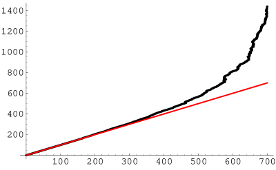
Figure 3: Left: The node number as a function of the support size of the minimizer at that node. At first these increase equally (straight line), but, as the remainder approaches zero, the number of nodes increases faster than the number of nonzero components in the minimizer. At the end there are more than twice as many nodes as there are nonzero components in $\bar{x}$. Right: The relative error $\|\bar{x}-S_{\lambda}(\bar{x}+K^{T}(y-K\bar{x}))\|/\|\bar{x}\|$ as a function of the node number for the same example. Ideally this should be zero as the minimizers are supposed to satisfy the fixed point equation (8). Due to numerical round-off it is not exactly zero. The matrix $K$ and data $y$ were chosen at random (see text).

6 Summary

A Mathematica package for the minimization of $\ell_{1}$ penalized functionals was described.

The FindMinimizer algorithm finds the exact minimizer of such a functional, as long as exact input is given. For floating point data, the same algorithm can be used to obtain a (very good) numerical approximation of the minimizer.

The FindMinimizer algorithm also handles the case of different penalties for different components: $\lambda\sum_{i}w_{i}|x_{i}|$ instead of $\lambda\|x\|_{1}$, including the case where some of the $w_{i}$ are zero.
In [20], a wavelet basis is used together with the iterative soft-thresholding algorithm (15) to perform denoising. A wavelet decomposition consists of wavelet coefficients (encoding local detail) and scaling coefficients (encoding large scale averages). This is an example where it makes very good sense to penalize different components differently or not to penalize (at all) the scaling coefficients. A geophysical example of the use of such a technique in seismology can be found in [21].

In many ways, this FindMinimizer algorithm is an improvement over the Matlab implementation [19, 17]; the latter cannot handle exact numbers (integer, rational), cannot handle zero weights, and sometimes does not give the correct answer (see the fourth example in section 5). The present algorithm can also compile a list of intermediate results on the fly. The intermediate value of $x$, $y-Kx$ and $K^{T}(y-Kx)$ have to be computed anyway; if one would do this after finishing the algorithm (based on a list of the nodes), one has to perform a great number of matrix multiplications all over again thereby doubling the computing time. Also, it might be impossible to store all the intermediate minimizer nodes, rendering the latter strategy impossible in certain cases. Again, this is not possible with [17, 19] (it only outputs a list of all the intermediate minimizers).
Also with regard to the possible stopping conditions, the present algorithm has more possibilities: [19] can stop at a predetermined number of nonzero components, or at a predetermined 1-norm of the minimizer. SolveLasso in SparseLab [17] can stop at the first breakpoint with penalty parameter or discrepancy below a predefined level (though no interpolation with the previous breakpoint is done to arrive at the exact value) or after a given number of steps. FindMinimizer has a generic stopping condition but can also stop at a predetermined value of the penalization parameter $\lambda$, of $\|\bar{x}\|_{1}$ or at a specific value of the discrepancy $\|K\bar{x}-y\|^{2}$ exactly. The latter is very useful in practice when using the so-called discrepancy principle [22]: the minimizer should not fit the data better than the level of the measurement noise.

The FindMinimizer algorithm was tested on hundreds of thousands of randomly generated matrices and data (both square and rectangular). The results were verified and no wrong outcomes were discovered. This is no guarantee that there aren’t any bugs left. Hence, it is recommended that users would check the results returned by the algorithms by checking equations (7) or (11).

The FindMinimizer function does not give a warning when the solution is not unique. If using floating point numbers and a warning about ill-conditioned matrix is generated, this may mean that the minimizer is not unique.

The worst case scenario for the FindMinimizer procedure happens when the first remainder $K^{T}y$ has all components of the same size. In this case, the algorithm has to resort to trying all possibilities to determine the new index/indices (there are $2^{n}-1$ nonempty subset of $\{1,2,\ldots,n\}$). Such a special case ‘never’ happens in practice, but it is easy to manually construct such examples.

Five other useful algorithms, like the iterative soft-thresholding algorithm (15) and algorithms that use projection on an $\ell_{1}$-ball (see expressions (16–19)) are also implemented. They also support the use of (zero and nonzero) weights. In general, after a finite number of steps, these only yield an approximative minimizer.

For clarity, only examples with very small size matrices were given in this manuscript. However, the package was also tested on the geo-physics application discussed in [21], and FindMinimizer succeeded in performing that minimization in less than one minute. The package was also used to evaluate the performance of competing iterative methods (other than the ones also discussed here) [23]. The comparison of the relative strength and weaknesses of these different algorithms lies beyond the scope of this work.
Quite a number of other methods for finding the minimizer (3) are available in SparseLab [17]. Some are designed to find the related $\arg\min_{Kx=y}\|x\|_{1}$ instead of (3). The $\ell_{1}$-magic package [18] also provides a number of primal-dual interior point methods for solving this and related problems in Matlab; it does not have an implementation for the Lasso/homotopy method.

Future work consists of extending the exact algorithm to the case of linearly constrained minimization:

$$\min_{x}\|Kx-y\|^{2}+2\lambda\|x\|_{1}\qquad\mathrm{with}\quad Ax=a,$$ (20)

i.e. minimization of the same $\ell_{1}$ penalized least squares functional as before, but now under additional linear constraint(s) described by the linear equation(s) $Ax=a$. Although approximative methods do exist for this problem, a LARS/homotopy-style (exact) method for constrained minimization was not described in [14, 15]. It is possible to solve this problem exactly and a prototype of such an exact algorithm, based on the FindMinimizer algorithm, has already been implemented and used in an application of portfolio construction (in finance) [24].

7 Acknowledgements

Most of the work presented in this article was done while the author was a ‘Francqui Foundation intercommunity post-doctoral researcher’ at the Université Libre de Bruxelles. Part of this work was done as a post-doctoral research fellow for the F.W.O-Vlaanderen (Belgium) at the Vrije Universiteit Brussel. Financial help was also provided by VUB-GOA 62 grant. Stimulating discussions with I. Daubechies and C. De Mol are gratefully acknowledged. The author thanks the referees for their suggestions which greatly helped improve the manuscript.

References

- [1] M. Bertero, Linear inverse and ill-posed problems, in: P. W. Hawkes (Ed.), Advances in Electronics and Electron Physics, Vol. 75, Academic Press, 1989, pp. 1 –120.
- [2] H. Engl, M. Hanke, A. Neubauer, Regularization of inverse problems, in: Mathematics and Its Applications, Vol. 375, Kluwer, 1996.
- [3] M. Bertero, P. Boccacci, Introduction to inverse problems in imaging, Institute of Physics, Bristol, 1998.
- [4] R. Tibshirani, Regression shrinkage and selection via the lasso, J. Royal. Statist. Soc B. 58 (1996) 267–288.
- [5] F. Santosa, W. W. Symes, Linear inversion of band-limited reflection seismograms, SIAM J. Sci. Stat. Comput. 7 (1986) 1307–1330.
- [6] S. S. Chen, D. L. Donoho, M. A. Saunders, Atomic decomposition by basis pursuit, SIAM J. Sci. Comput. 20 (1) (1998) 33–61.
- [7] D. Donoho, Compressed sensing, Information Theory, IEEE Transactions on 52 (4) (2006) 1289–1306.
- [8] E. J. Candès, J. K. Romberg, T. Tao, Stable signal recovery from incomplete and inaccurate measurements, Communications on Pure and Applied Mathematics 59 (8) (2006) 1207–1223.
- [9] I. Daubechies, M. Defrise, C. De Mol, An iterative thresholding algorithm for linear inverse problems with a sparsity constraint, Communications On Pure And Applied Mathematics 57 (11) (2004) 1413–1457.
-
[10]
I. Daubechies, M. Fornasier, I. Loris, Accelerated projected gradient method
for linear inverse problems with sparsity constraints, To appear in Journal
of Fourier Analysis and Applications.
URL http://arxiv.org/abs/0706.4297 -
[11]
K. Koh, S.-J. Kim, S. Boyd, A method for large-scale l1-regularized least
squares problems with applications in signal processing and statistics
(2007).
URL http://www.stanford.edu/~boyd/l1_ls/ - [12] M. A. T. Figueiredo, R. D. Nowak, S. J. Wright, Gradient projection for sparse reconstruction: Application to compressed sensing and other inverse problems, IEEE Journal of Selected Topics in Signal Processing (Special Issue on Convex Optimization Methods for Signal Processing), 1 (2007) 586–598.
- [13] C. Chaux, P. L. Combettes, J.-C. Pesquet, V. R. Wajs, A variational formulation for frame-based inverse problems, Inverse Problems 23 (4) (2007) 1495–1518.
- [14] M. R. Osborne, B. Presnell, B. A. Turlach, A new approach to variable selection in least squares problems, IMA J. Numer. Anal. 20 (3) (2000) 389–403.
- [15] B. Efron, T. Hastie, I. Johnstone, R. Tibshirani, Least angle regression, Ann. Statist. 32 (2) (2004) 407–499.
- [16] Mathematica: Version 5.2, Wolfram Research Inc., Champaign, Illinois, 2005.
-
[17]
D. Donoho, V. Stodden, Y. Tsaig, About SparseLab (March 2007).
URL http://sparselab.stanford.edu/ -
[18]
E. Candès, J. Romberg, -magic : Recovery of sparse signals via
convex programming (October 2005).
URL http://www.acm.caltech.edu/l1magic/index.html -
[19]
K. Sjöstrand, Matlab implementation of LASSO, LARS, the elastic net
and SPCA, version 2.0 (jun 2005).
URL http://www2.imm.dtu.dk/pubdb/p.php?3897 - [20] M. Figueiredo, R. Nowak, An EM algorithm for wavelet-based image restoration, Image Processing, IEEE Transactions on 12 (8) (2003) 906–916.
-
[21]
I. Loris, G. Nolet, I. Daubechies, F. A. Dahlen, Tomographic inversion using
-norm regularization of wavelet coefficients, Geophysical Journal
International 170 (1) (2007) 359–370.
URL http://arxiv.org/abs/physics/0608094 - [22] M. Defrise, C. De Mol, A note on stopping rules for iterative regularization methods and filtered svd, in: P. C. Sabatier (Ed.), Inverse Problems: An interdisciplinary Study, Academic Press, 1987, pp. 261–268.
-
[23]
I. Loris, On the performance of algorithms used for the minimization of
-penalized functionals, Submitted to Journal Of Physics Conference
Series.
URL http://arxiv.org/abs/0710.4082 -
[24]
J. Brodie, I. Daubechies, C. De Mol, D. Giannone, I. Loris, Sparse and stable
Markowitz portfolios, Preprint.
URL http://arxiv.org/abs/0708.0046