A universal GRB photon energy-peak luminosity relation

Abstract

The energetics and emission mechanism of GRBs are not well understood. Here we demonstrate that the instantaneous peak flux or equivalent isotropic peak luminosity, $L_{iso}$ ergs s^-1, rather than the integrated fluence or equivalent isotropic energy, $E_{iso}$ ergs, underpins the known high-energy correlations. Using new spectral/temporal parameters calculated for 101 bursts with redshifts from BATSE, BeppoSAX, HETE-II and Swift we describe a parameter space which characterises the apparently diverse properties of the prompt emission. We show that a source frame characteristic-photon-energy/peak luminosity ratio, $K_{z}$, can be constructed which is constant within a factor of 2 for all bursts whatever their duration, spectrum, luminosity and the instrumentation used to detect them. The new parameterization embodies the Amati relation but indicates that some correlation between $E_{peak}$ and $E_{iso}$ follows as a direct mathematical inference from the Band function and that a simple transformation of $E_{iso}$ to $L_{iso}$ yields a universal high energy correlation for GRBs. The existence of $K_{z}$ indicates that the mechanism responsible for the prompt emission from all GRBs is probably predominantly thermal.

1 Introduction

The energetics of the central engine which powers the explosion responsible for a GRB are both intriguing and fundamental to our understanding of these cosmic events. The isotropic energy outflow at source, estimated using the integrated gamma-ray fluence, is enormous, up to $E_{iso}\sim 10^{54}$ ergs, and even if the outflow is collimated in jets the total energy involved is still huge, $E_{\gamma}\sim 10^{51}$ ergs. The possibility that the explosion taps a standard energy resevoir has been pursued by many authors following the initial suggestion from Frail et al. (2001). If this total energy available were, indeed, roughly constant (or predictable through other means) and we could reliably estimate the collimation, then GRBs could be used as a cosmological probe to very high redshifts, Bloom et al. (2003), Ghirlanda et al. (2004).

Early on it was noted that, based on analysis of BATSE data, there was a correlation between $E_{p}$, the peak of $E.F(E)$ where $F(E)$ ergs cm^-2 keV^-1 is the observed spectrum, and the fluence (Mallozzi et al. 1995, Lloyd et al. 2000). When redshifts became available for long bursts the isotropic energy, $E_{iso}$, could be estimated from the fluence and the peak energy could be transformed into the source frame, $E_{pz}$, the so-called Amati relation, a correlation between $E_{iso}$ and $E_{pz}$ in the sense that more energetic bursts have a higher $E_{pz}$, was discovered using data from BeppoSAX, (Amati et al. 2002). This correlation has subsequently been confirmed and extended although there remain many significant outliers, including all short bursts. The physical origin of the correlation may be associated with the emission mechanisms operating in the fireball but the theoretical details are far from settled (see the discussion by Amati (2006) and references therein). More recently a tighter correlation between $E_{iso}$, $E_{pz}$ and the jet break time, $t_{break}$, measured in the optical afterglow has been reported (Ghirlanda et al. 2004). This is explained in terms of a modification to the Amati relation in which $E_{iso}$ is corrected to a true collimated energy, $E_{\gamma}$, using an estimate of the collimation angle derived from $t_{break}$. The details of the collimation correction depend on the density and density profile of the circumburst medium, Nava et al. (2006) and references therein. Multivariable regression analysis was performed by Liang & Zhang (2005) to derive a model-independent relationship, $E_{iso}\propto E_{pz}^{1.94}t_{zbreak}^{-1.24}$, indicating that the rest-frame break time of the optical afterglow, $t_{zbreak}$ was indeed correlated with the prompt emission parameters.

Other studies have concentrated on the properties of the isotropic peak (maximum) luminosity, $L_{iso}$ ergs s^-1, measured over some short time scale $\approx 1$ s, rather than the time integrated isotropic energy, $E_{iso}$. Yonetoku et al. (2004) noted a correlation between $L_{iso}$ and $E_{pz}$ for 16 GRBs with firm redshifts. A correlation between $L_{iso}$ and the spectral lag was first identified by Norris et al. (2000) and explained in terms of the evolution of $E_{peak}$ with time. The shocked material responsible for the gamma-ray emission is expected to cool at a rate proportional to the gamma-ray luminosity and it has been suggested that $E_{peak}$ traces the cooling (Schaefer 2004). A similar correlation between $L_{iso}$ and the variability of the GRB ($V$) was described by Reichart et al. (2001). The origin of the $L_{iso}-V$ relation is likely to be related to the physics of the relativistic shocks and the bulk Lorentz factor of the outflow. It could be that high $\Gamma_{outflow}$ results in high $L_{iso}$ and $V$ while lower luminosity and variability are expected if $\Gamma_{outflow}$ is low (see, for example, Mészáros et al. 2002). A rather bizzare correlation involving $L_{iso}$, $E_{pz}$ and variability was found by Firmani et al. (2006). They employed the “high signal” time, $T_{45}$, as formulated by Reichart et al. (2001) in their study of variability, and showed that $L_{iso}\propto E_{pz}^{1.62}T_{45}^{-0.49}$ for 19 GRBs with a spread much narrower than that of the Amati relation. There is currently no explanation for such a correlation although it may be connected with the spectral lag and variability correlations and the Amati relation.

The correlation between $E_{iso}$ and $E_{pz}$ supplemented by additional empirical information can be used in pseudo redshift indicators, for example Atteia (2003), Pelangeon & Atteia (2006), but the intrinsic spread in the correlation and uncertainty about the underlying physical interpretation introduce errors, typically of a factor $\sim 2$. It may be possible to reduce the errors by simultaneous application of several independent luminosity/energy correlations, and extension of the Hubble Diagram to high redshifts using GRBs has been attempted, see for example Schaefer (2007). However, it is not clear that the correlations briefly described above are truly independent and there may be some underlying principle or mechanism which connects them all together. Recently, and more controversially, Butler et al. (2007) have raised serious doubts about the validity of these correlations suggesting that it is likely that they are introduced by observational/instrumental bias and have nothing to do with the physical properties of the GRBs and hence they conclude that GRBs are probably useless as cosmological probes. Here we take a new look at the source frame spectral and temporal properties of a large number of GRBs for which we have redshifts in order to try and understand what really correlates with what and whether or not this can provide useful intrinsic information about the GRBs and what drives them. In this analysis we include the short-duration GRBs which may share a similar emission mechanism with long bursts despite probably having different progenitors.

2 Source frame spectra of the prompt emission

The profile of the prompt energy spectrum of all GRBs is well represented by a Band function (Band et al. 1993),

$$B(E)=E^{-\beta_{X}}\exp(-E/E_{c}),\>\>E\leq E_{c}(\beta_{\gamma}-\beta_{X})$$

$$B(E)=E^{-\beta_{\gamma}}\exp(\beta_{\gamma}-\beta_{X})[(\beta_{\gamma}-\beta_{X})E_{c}]^{\beta_{\gamma}-\beta_{X}},\>\>E\geq E_{c}(\beta_{\gamma}-\beta_{X})$$ (1)

where $\beta_{X}$ and $\beta_{\gamma}$ are the spectral power law indices at low (X-ray) and high ($\gamma$-ray) energies respectively and $E_{c}$ keV is the high cut-off energy. Note that in the original formulation of Band et al. (1993) photon indices were used and the profile described the photon number density (because these are the parameters which most closely describe the detected count spectrum which is fitted). Here we choose to use an energy density profile and energy spectral indices. The observed total fluence is

$$F_{tot}=\int_{E_{1}}^{E_{2}}F(E)dE=N_{tot}\int_{E_{1}}^{E_{2}}B(E)dE$$ (2)

ergs cm^-2, where $N_{tot}$ is the normalisation in ergs cm^-2 keV^-1 at 1 keV and $E_{1}$ to $E_{2}$ is the observed energy band. Spectral fitting of the observed count spectrum will yield values for $\beta_{X}$, $\beta_{\gamma}$, $E_{c}$ and $N_{tot}$. The cut-off energy, $E_{c}$, is often converted to the peak energy of the $E.F(E)$ spectrum which is given by $E_{p}=(1-\beta_{X})E_{c}$ and the normalisation may be expressed as the fluence, $F_{tot}$, rather than the energy density at 1 keV, $N_{tot}$. However, the separation of the fluence into a normalisation term and a spectral integral is central to the development of the argument which follows. Table 1 gives the spectral parameters for 101 GRBs for which we have redshift values and a prompt light curve. The spectral parameters for bursts detected by BATSE, BeppoSAX, HETE-2 and Konus/WIND were taken from the references cited. The values for Swift bursts were derived from the BAT spectra supplemented by detections by INTEGRAL and Konus/WIND where available. Many of the Swift spectra ($\approx 40$) are adequately fitted by a simple power law or a cut-off power law with $E_{c}$ fixed. For these bursts a cut-off power law model was used with $E_{c}=150$ keV (corresponding to the upper limit of the BAT energy band). Providing the fitted $\beta_{X}<1$ the fitted function has a peak in $E.F(E)$ and a value for the peak energy can then be estimated. The spectra of 7 very soft Swift bursts with redshifts (GRB050406, GRB050416A, GRB050824, GRB051016B, GRB060512, GRB060926 and GRB070419A) gave $\beta_{X}\geq 1$ and these were discarded because, for such spectra, we have no meaningful estimate of $E_{p}$. Such GRBs are normally designated as X-ray flashes (XRFs) and the exceptionally high $\beta_{X}$ values may arise because we are actually observing the high energy tail ($\beta_{\gamma}$) and not the lower energy power law in the Band function. Alternatively it may be that such soft spectra are the result of a second soft X-ray component which dominates in these objects.

The equivalent isotropic energy from the source is given by

$$E_{iso}=\frac{4\pi d_{L}^{2}N_{tot}}{(1+z)^{2-\beta_{X}}}I_{bol}(E_{pz},\beta_{X},\beta_{\gamma})$$ (3)

ergs, where $d_{L}$ is the luminosity distance corresponding to the redshift $z$ under some cosmology, $I_{bol}(E_{pz},\beta_{X},\beta_{\gamma})$ is the bolometric integral of the spectral energy profile in the source frame, $B_{z}$, taken over the wide energy band 1 keV to 10 MeV

$$I_{bol}(E_{pz},\beta_{X},\beta_{\gamma})=\int_{1}^{10^{4}}B_{z}(E)dE$$ (4)

and $E_{pz}=E_{p}(1+z)$ is the peak energy in the source frame. The first term in Equation 3 is the equivalent isotropic energy density, $Q_{z}$ ergs keV^-1 at 1 keV in the source frame.

$$Q_{z}=\frac{4\pi d_{L}^{2}N_{tot}}{(1+z)^{2-\beta_{X}}}.$$ (5)

A factor $1/(1+z)^{1-\beta_{X}}$ arises because we have shifted the normalisation from 1 keV in observer frame to 1 keV in the source frame. The remaining factor of $1/(1+z)$ accounts for the time-dilation of the duration over which the bursts are seen. It is pertinent to transform this to the isotropic energy density at the peak energy, $E_{pz}$ keV, in the source frame,

$$Q_{pz}=Q_{z}\exp[(1-\beta_{X})(E_{pz}^{-1}-1)]E_{pz}^{-\beta_{X}}$$ (6)

ergs keV^-1 so that the spectrum normalisation is specified at a characteristic energy in or close to the observed $\gamma$-ray energy band. We can then write Equation 3 as

$$E_{iso}=Q_{pz}E_{wz},$$ (7)

where

$$E_{wz}=\exp[(\beta_{X}-1)(E_{pz}^{-1}-1)]E_{pz}^{\beta_{X}}I_{bol}(E_{pz},\beta_{X},\beta_{\gamma})$$ (8)

keV is a characteristic photon energy which depends on the profile of the energy spectrum and the limits adopted for the integration and it serves to convert from an energy density ($Q_{pz}$ ergs keV^-1) at the peak of the $E.F_{z}(E)$ spectrum to the total isotropic energy ($E_{iso}$ ergs). The isotropic energy spectrum in the source frame is given by

$$F_{z}(E)=Q_{z}B_{z}(E)=Q_{pz}\exp[(\beta_{X}-1)(E_{pz}^{-1}-1)]E_{pz}^{\beta_{X}}B_{z}(E)$$ (9)

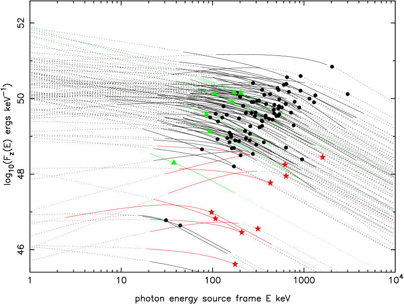
Figure 1: The 1 keV to 10 MeV source frame spectra of GRBs listed in Table 1. The observed energy band is shown as the solid line in each case. $Q_{pz}$ values are marked; solid dots for long GRBs, solid stars for short GRBs and solid triangles for XRFs.

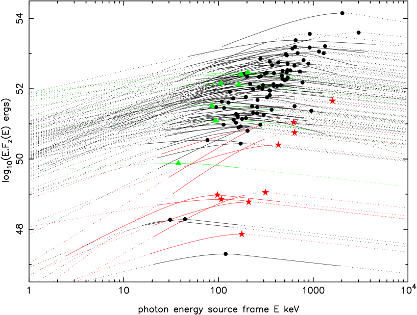
Figure 2: The 1 keV to 10 MeV $E.F_{z}(E)$ source frame spectra of GRBs listed in Table 1. The observed band is shown as the solid line in each case. $E_{pz}Q_{pz}$ values are marked at the peak energy $E_{pz}$; solid dots for long GRBs, solid stars for short GRBs and solid triangles for XRFs.

ergs keV^-1. The source frame spectra of the GRBs listed in Table 1 are shown in Figure 1 with the spectral energy density $Q_{pz}$ marked at energy $E_{pz}$ keV. In the majority of spectra the high energy spectral index is not measured but set to $\beta_{\gamma}=1.3$ which is the approximate average found by BATSE. Figure 2 shows the corresponding $E.F_{z}(E)$ spectra in ergs. We assumed a cosmology with $H_{0}=71$ km s^-1 Mpc^-1, $\Lambda=0.27$ and $\Omega=0.73$ to calculate the luminosity distance $d_{L}$.

3 The Amati relation

The Amati relation is a correlation between $E_{pz}$ and $E_{iso}$, first reported by Amati et al. (2002), and subsequently shown to be obeyed by the majority of long GRBs although there is a fairly large scatter. The top left panel of Figure 3 shows the histogram of isotropic energy values, $E_{iso}$, calculated using Equation 7 using the spectral parameters in Table 1 and redshift in Table 3. A large range of values for $E_{iso}$ is produced because of the spread in the isotropic energy density at the peak $Q_{pz}$, the peak energy $E_{pz}$ and the bolometric integral $I_{bol}$. The top right panel of Figure 3 shows the peak energy values, $E_{pz}$, plotted against the characteristic energy, $E_{wz}$. There is a tight correlation between these 2 parameters because of the form of the Band function. To a first approximation $E_{pz}=0.23E_{wz}$ (the solid line in Figure 3) although the best fit correlation is a little steeper ($E_{pz}\propto E_{wz}^{1.14}$) and the small scatter evident in Figure 3 is introduced by differences in the spectral indices, $\beta_{X}$ and $\beta_{\gamma}$. In fact, the bolometric integral is well approximated by a function of the form

$$I_{bol}\approx I_{fit}=E_{pz}^{1+c_{1}}\exp(c_{0}+c_{2}\beta_{X}+c_{3}\beta_{\gamma})$$ (10)

where the coefficients $c_{0},c_{1},c_{2},c_{3}$ can be found by a least squares fitting procedure. A comparison of $I_{fit}$ and $I_{bol}$ for the GRBs listed in Table 1 is shown in the bottom left panel of Figure 3 together with the best fit coefficients. We can use $I_{fit}$ in place of $I_{bol}$ and estimate $E_{iso}\approx E_{fit}$. The distribution of the ratio $E_{iso}/E_{fit}$ is shown in the bottom right-hand panel of Figure 3. For the majority of objects the estimation, $E_{fit}$, is within $\pm 10\%$ of the value obtained by numerical integration. There are a few GRBs with a larger discrepancy but all are within $\pm 20\%$ which is a very small perturbation in comparison with the dynamic range of the $E_{iso}$ values.

Using $I_{bol}\approx I_{fit}$ we can express $E_{iso}$ as an explicit function of $E_{pz}$:

$$E_{iso}\approx Q_{pz}E_{pz}^{\beta_{X}+1+c_{1}}\exp(1+c_{0}+(c_{2}-1)\beta_{X}+c_{3}\beta_{\gamma}).$$ (11)

The immediate origin of the Amati relationship is now clear. Given Equation 11 some degree of correlation between $E_{pz}$ and $E_{iso}$ is guaranteed. The nature and spread of this correlation will depend on the relationship between the flux density, $Q_{pz}$, and the peak energy, $E_{pz}$, and the distribution of spectral index $\beta_{X}$. It could be that $Q_{pz}$ and $E_{pz}$ are correlated in such a way to cancel the apparent dependence on $E_{pz}$ but this is highly unlikely. This correlation arises because the GRB spectral profile has the form of Band function (Equation 1) with a particular range of values for the spectral indices, $\beta_{X}$, $\beta_{\gamma}$, and the energy $E_{c}$. So understanding where the Amati relation comes from is really the same as understanding why the spectra have this functional form in the first place.

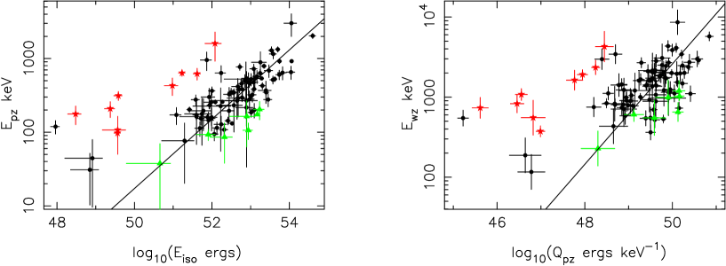
Figure 4: Left-hand panel: The Amati relation for the GRBs in Table 1. Right-hand panel: $E_{wz}$ vs. $Q_{pz}$ for the same GRBs. Solid dots for long GRBs, solid stars for short GRBs, solid triangles for XRFs.

Figure 4 shows the Amati relationship for the GRBs in Table 1. Here and subsequently we use the exact form for $E_{iso}$, calculated from $I_{bol}$, and not the approximation involving $I_{fit}$ which was only introduced to derive Equation 11. The correlation line shown (derived ignoring the obvious outliers) is $E_{pz}\propto E_{iso}^{0.46}$ consistent with Amati 2006, $E_{pz}\propto E_{iso}^{0.5}$. All the short bursts are outliers with low $E_{iso}$ values compared with the long bursts of similar $E_{pz}$ value. The other notable outliers are GRB980425 and GRB060218 (see Amati 2006, Campana et al. 2006). The XRFs (characterised by the hardness ratio of the low energy spectra, see below) all fall on the lower edge of the correlation with low $E_{pz}$ compared with $E_{iso}$. A more fundamental relationship is that between the flux density $Q_{pz}$ and the characteristic energy $E_{wz}$ which is also shown in Figure 4. It appears that, disregarding the short bursts, the Amati correlation is tighter than this new relationship but this is deceptive. Unlike $E_{iso}$ and $E_{pz}$, $Q_{pz}$ and $E_{wz}$ are independent and their product provides the isotropic energy $E_{iso}$ (Equation 7). We now have a correlation which goes beyond the simple fact that GRB spectra have the Band function profile. Crudely, $Q_{pz}$ is a measure of the height of the spectrum as plotted in Figure 1 and $E_{wz}$ (which is itself a function of $E_{pz}$, $\beta_{X}$ and $\beta_{\gamma}$) is a measure of the characteristic photon energy. There is a weak correlation between these two quantities, $E_{wz}\propto Q_{pz}^{0.3}$, as can be seen in Figures 4 and 1. However, the pattern of outliers is the same as for the Amati relationship. The short bursts, and the sub-luminous long burst, GRB980425, have significantly low $Q_{pz}$ values but $E_{wz}$ values which are comparable to the gamut of long bursts. The bursts designated as XRFs (see below) all lie in the low tail of the $E_{wz}$ range but have $Q_{pz}$ values which are similar to many long bursts.

4 The rate profile and luminosity time of the prompt emission

The analysis above has highlighted the well known problems associated with the Amati relation and other correlations involving $E_{iso}$. We now consider a way of converting $E_{iso}$ into a characteristic luminosity to see if this can improve the situation. The variety of time variablity in the prompt emission from GRBs is astonishing. Some bursts consist of a single Fast Rise Exponential Decay (FRED) profile, other have multiple peaks, some are very spikey with rapid variations while others have a smoother profile. The luminosity is continually varying between bright, short peaks and low troughs and in some cases the flux drops below the detection threshold for a while before flaring up again. With such a range of behaviour defining some characteristic luminosity and/or duration is tricky. Reichart et al. (2001) showed that the peak luminosity correlated with a variability measure $V$ computed by taking the difference between the light curve and a smoothed version of the light curve where the smoothing or correlation time was the time taken to emit the brightest fraction $f$ of the flux, $T^{E}_{f}$. They showed that the most robust correlation was obtained for $f\approx 0.45$. The correlation of the peak luminosity with $T_{45}$ has been adopted by subsequent authors, for example Guidorzi et al. (2005), Firmani et al. (2006), but in all cases the peak luminosity must be defined using some small arbitrary bin size (typically 1 second) and the only connection between the total fluence and the peak luminosity is indirect, through the $T_{45}$ value.

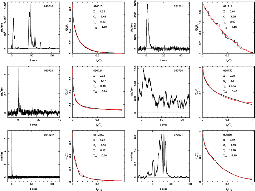
Figure 6: Typical prompt emission light curves and the corresponding rate profiles. The light curves have been smoothed with a boxcar function of width $T_{45}$ for display purposes.

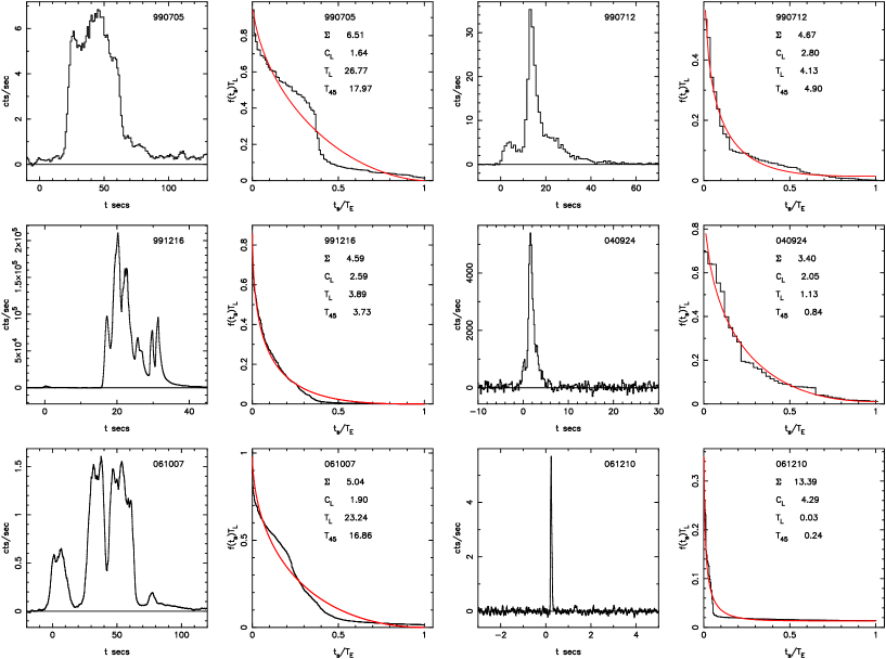
Figure 8: Light curves and the corresponding rate profiles for which the fit statistic $\Sigma$ is high. The light curves have been smoothed with a boxcar function of width $T_{45}$ for display purposes.

The variability measure $V$ depends on the correlation of structures (peaks, troughs etc.) in the light curves. Here we try a different approach in which the sequence of features or events in the light curves is abandoned completely. We identify the time periods in which significant flux is measured and then construct a rate profile by sorting the sequence of count rate samples from these time periods into descending order to produce, for every GRB, a monotonically decreasing function, $f_{s}(t_{s})$, where $t_{s}$ is sorted time. The total sum of all the samples should be the total count fluence and the profile is normalised by dividing by this fluence so that the integral under the profile is unity. Such a rate profile shows what fraction of the burst is spent at what fraction of the peak rate and has the general form shown schematically in Figure 5. Examples of these rate profiles are shown in Figures 6 and 8. The time periods in which significant flux is detected were found by successive correlation with boxcar functions of increasing width. It doesn’t matter if the total duration of these periods is a little larger than required to capture the total fluence because the small excess of samples in the tail can be dropped and the rest of the profile is unchanged. Remarkably the shape of these rate profiles is surprisingly similar for all GRBs and is insensitive to the time bin size used as long as it is not too large or too small. If the bin size is too large then there may be too few samples defining the profile, but we found that a number of bins $>20$ was fine. Using excessively large time bins can also hide significant real structure in the fluctuations of the light curve and this should be avoided. At the other extreme, if the bins are too small the number of counts per bin may drop to single figures and the profile shape is again compromised. In practice all long bursts are well represented using $\approx 64$ ms bins while short bursts require $\approx 4$ ms bins or something similar.

The influence of statistical fluctuations (noise) on the rate profiles is rather strange. Because the integral is normalised to unity statistical fluctuations on the total fluence are not included. The profile reflects the distribution of the detected flux over a range of brightness but is not influenced by uncertainties in the total flux. The sorting of bins into decreasing brightness order also ensures the profiles are always smooth with the larger errors or distortion due to noise accumulating at the start and end of the profile. This is often most noticable as a slight increase in gradient or curl over at the end of the profile. Although errors can be estimated for each of the samples, $d_{i}$, Chi-squared minimization using these errors cannot be employed for any function fitting because the sorting operation destroys the meaning of the errors. i.e. the scatter of the sorted data values about the fitted function is not governed directly by the errors on $d_{i}$.

Most profiles are well represented by an empirical function of the form

$$f_{s}(t_{s})=f_{0}\left(1-\left(\frac{t_{s}}{T_{E}}\right)^{1/C_{L}}\right)^{C_{L}}+f_{E}$$ (12)

where $T_{E}$ is the total emission time or duration of the profile, $f_{E}$ is the level of the profile at $T_{E}$ and represents the minimum detectable flux (or luminosity) and $C_{L}$ is a luminosity index which describes the curvature. This function is illustrated in Figure 5. Because the profile integral is normalised to unity the peak value at the start is $f_{0}+f_{E}=1/T_{L}$, where $T_{L}$ is a luminosity time in seconds. The peak flux is then given by the fluence divided by the luminosity time, $F_{tot}/T_{L}$ cts s^-1 or, perhaps more intuitively, the peak flux multiplied by $T_{L}$ is the total fluence. Because $T_{L}$ is derived from the functional fit of all the data it does not depend strongly on the time bin size (as discussed above) and therefore the peak flux calculated using $T_{L}$ is also not dependent on the binning. If $C_{L}=1$ the profile is linear and if $C_{L}>1$ the profile is concave and the fraction at high rate is smaller. If $C_{L}<1$ the curvature would be negative but this is not seen for any GRBs. So $C_{L}$ is a measure of the sharpness or spikiness of the profile.

We fitted all rate profiles with the function $f_{s}$ given by Equation 12 finding the best fit values for the parameters $T_{L}$, $C_{L}$ and $f_{E}$ using a least squares statistic

$$\Sigma=100N\Delta t^{2}\sum(d_{i}-f_{si})^{2}$$ (13)

where $N$ is the total number of samples, $d_{i}$, of time width $\Delta t$. Note $T_{E}$ is fixed as the cumulative duration of all the significant samples detected, $T_{E}=N\Delta t$. The $\Sigma$ statistic has properties similar to reduced Chi-Squared, with typical values in the range 0.5-2.0 (set by the scaling factor of 100), independent of the number of samples $N$ or the sample size $\Delta t$. Table 2 provides a complete list of all the temporal parameters. This table also includes the instrument and a GRB classification using the usual observational definitions: Short bursts if $T_{90}<2$ s and X-ray Flashes (XRFs) if fluence(1-30 keV)/fluence(30-500 keV)$>1$.

Figure 6 shows examples of typical fits. Note that sorted time is scaled by $1/T_{E}$ and the $f_{s}$ values by $T_{L}$ so that both axes take the range 0-1. The top-right panels show GRB021211 which is a typical FRED burst and has a low curvature index, $C_{L}=1.28$. The top-left and bottom right panels show GRB990510 and GRB070521 which have more complicated flaring structure but are well fitted with $C_{L}$ values of 2.48 and 1.69 respectively. The remaining objects have short bright spikes and extended low level emission, a class discussed by Norris & Bonnell (2006). GRB050724 and GRB051221A are essentially short bursts followed by a low level, extended tail and the combination of these features produces large $C_{L}$ values, 3.17 and 2.85 respectively. For GRB051221A, $\Sigma=3.22$ which is rather high. In this case the short spike followed by the extended tail produces an extra feature or wiggle in the rate profile which is not fitted by the simple $f_{s}$ function, Equation 12. For these and similar bursts a sample size of 4 ms was used to accomodate the profile of the initial short spike. The left-hand panel of Figure 7 shows the distribution of $\Sigma$ and $T_{L}$ values for all GRBs in Table 2. There is no correlation between the goodness of fit measured by $\Sigma$ and the luminosity time, $T_{L}$. The same is true for $\Sigma$ and the luminosity index $C_{L}$. Figure 8 shows the worst fits of rate profiles with large $\Sigma$ values. In all these GRBs the peak value, $1/T_{L}$, is a good approximation to the data peak but the fit is compromised by undulating features. GRB990705 and GRB061007 represent a small group of bursts which have flares that rise fast, are reasonably flat at the top and decay fast. These produce a characteristic S-feature in the profile. Only 12 rate profiles (out of 101) have $\Sigma>2$ and only 3 of these have a substantial mis-match, GRB990705, GRB061007 and GRB061210. The latter is an extreme example of a short burst, $T_{L}=0.03$ s, which has an extended low flux tail giving $T_{90}=85.3$ s. We note that GRB991216 has a faint pre-cursor just visible on the lightcurve plot.

The combination of luminosity time, $T_{L}$, and curvature index, $C_{L}$, gives us information closely related to $T_{45}$. The right-hand panel of Figure 7 shows the correlation between $C_{L}$ and the ratio of $T_{45}$ calculated directly from the sample values $d_{i}$ and $T_{L}$ from the fitted function. $T_{45}$ could be calculated by integration of the fitted function using the parameters $T_{L}$, $C_{L}$, $f_{E}$ and $T_{E}$ and this would produce a smooth curve of $C_{L}$ vs. $T_{45}/T_{L}$ if $f_{E}$ were zero or constant. The parameter $C_{L}$, for example, could be replaced by $T_{45}$ and the fitted function would still be uniquely defined. The scatter in Figure 7 results from the small differences between the data and the fitted function and the value of $f_{E}$ which is generally much smaller than $1/T_{L}$ but different for each GRB. Error ranges for $T_{L}$ and $C_{L}$ were estimated assuming the statistic $\Sigma$ has properties similar to reduced Chi-Squared. The errors so derived are not statistically correct, because of the odd statistical nature of the sorted rate profile, and in some cases they are an over estimate as is evident from the scatter in Figure 7.

Although the minimum flux level, $f_{E}$, was included in the fitting it is a measure of the instrument sensitivity rather than some intrinsic property of the rate profile. If the noise level were lower the number of significant samples detected would increase, $T_{E}$ would get bigger and $f_{E}$ would decrease. The instrument would detect a slightly larger fluence, $F_{tot}$, and the fitted value of $T_{L}$ would increase a little, however, the peak flux level, $F_{tot}/T_{L}$ would remain unchanged and $C_{L}$ would be essentially the same. The analysis of the rate profile described above provides a robust estimate of the peak flux (or peak luminosity) using all the available light curve data and is not biased by the instrument sensitivity providing the burst detection significance is secure in the first instance. The error on the peak flux so estimated is dominated by the error on the fluence rather than any error associated with estimating the luminosity time, $T_{L}$. It is also unchanged by the choice of sample size, $\Delta t$, providing the number of samples is sufficient to capture the details of the emission profile as already discussed above. We can never be sure that resampling a light curve with a smaller $\Delta t$ will not reveal a very short, bright, isolated spike which was hidden by the previous binning and this would compromise the shape of the profile, but such has not been seen in any of the GRB light curves analysed so far (about 250 including all Swift bursts to date).

Using the redshift, $z$, we can calculate the luminosity time in the source frame, $T_{Lz}=T_{L}/(1+z)$ and $90\%$ duration in the source frame, $T_{90z}=T_{90}/(1+z)$. The peak luminosity multiplied by the $T_{Lz}$ gives the isotropic energy, $L_{iso}T_{Lz}=E_{iso}$ ergs. This simple property of $T_{Lz}$ makes it a highly significant measure of the burst duration and is why we chose to call it the luminosity time. Such a time is often introduced in theoretical dicussions, see for example $t_{j}$ in Thompson et al. (2007) or $t_{burst}$ in Ghirlanda et al. (2007). Above we have described a method to calculate this time for every GRB.

5 Characterisation of the prompt emission in the source frame

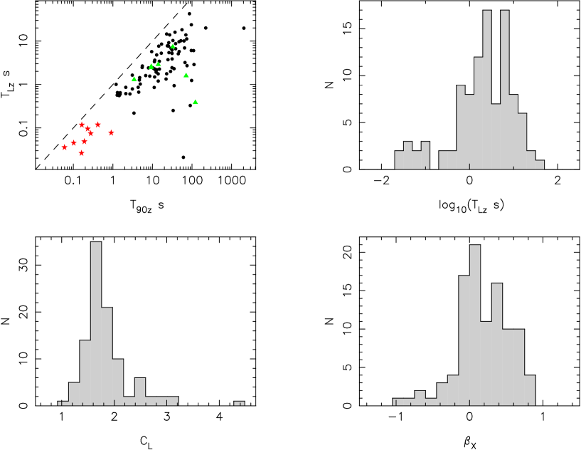
Figure 9: Top panels: The correlation between luminosity time $T_{Lz}$ and $T_{90z}$ and the distribution of $T_{Lz}$. The dashed line indicates the equality $T_{Lz}=T_{90z}$. Bottom panels: The distributions of $C_{L}$ and $\beta_{X}$ for the GRBs in Table 1.

The prompt emission of each GRB in the source frame is characterised by the peak energy density, $Q_{pz}$ ergs keV^-1, the characteristic photon energy, $E_{wz}$ keV (which embodies the spectral indices $\beta_{X}$, $\beta_{\gamma}$ and the peak energy $E_{pz}$, Equation 8), the luminosity time, $T_{Lz}$ s, and the luminosity curvature, $C_{L}$. Figure 9 shows $T_{Lz}$ plotted against the standard measure of burst length $T_{90z}$ where the dashed line shows equality. For bursts consisting of a single smooth pulse then $T_{Lz}\approx T_{90z}$. If there is more structure in the light curve and, in particular, if there are periods when the flux drops to zero then $T_{Lz}<T_{90z}$. In some cases a short precursor pulse is followed by a long time gap before the main burst starts and then $T_{Lz}<<T_{90z}$. So the ratio of the two times is a crude measure of the variability but this includes all time scales and long periods when no flux is detected and is not equivalent to the short time scale variability defined by Reichart et al. (2001). The top-right panel of Figure 9 shows the distribution of $T_{Lz}$. Two peaks containing the short-bursts, centred around 0.05 seconds, and long-bursts centred at 5 seconds, are clearly visible. The distribution of $C_{L}$ is shown in the lower left-hand panel of Figure 9. Most bursts are contained in a symmetrical peak centred on $C_{L}=1.6$. The few bursts with $C_{L}>2.2$ include the short bursts which have a long weak tail and bursts which exhibit several very short spikes on top of a more generally smooth emission. The bottom right-hand panel of Figure 9 shows the distribution of the Band lower energy spectral index, $\beta_{X}$. Hard bursts have $\beta_{X}<0$ and softer bursts have $\beta_{X}>0$. We do not show the distribution of the high energy spectral index, $\beta_{\gamma}$, because this parameter is only available for a few bursts and in most cases it was set to $\beta_{\gamma}=1.3$ which is the approximate average found by BATSE.

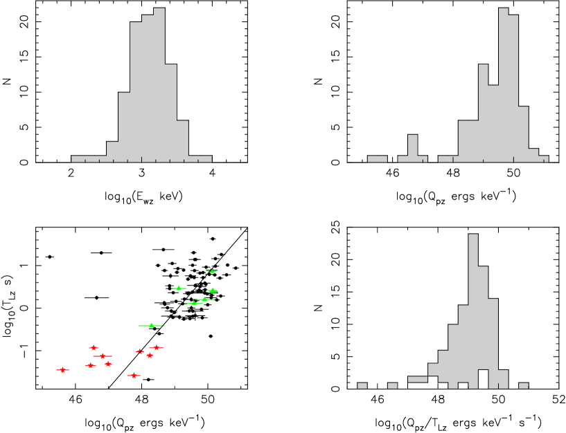
Figure 10: Top panels: The distributions of $E_{wz}$ keV and $Q_{pz}$ ergs keV^-1. Bottom panels: The correlation of $T_{Lz}$ s vs. $Q_{pz}$ and the distribution of the peak luminosity density, $Q_{pz}/T_{Lz}$ ergs keV^-1 s^-1. The distribution for short bursts is shown as the white histogram.

The distributions of the remaining parameters, the characteristic photon energy, $E_{wz}$, and the peak energy density, $Q_{pz}$, are shown at the top of the Figure 10. $E_{wz}$ stretches over two decades from 100 keV to 10000 keV. $Q_{pz}$ has a much larger spread with a main peak spanning three decades and a low energy tail covering another three. Since the product of the two gives us $E_{iso}$ the range of isotropic energy is very large, as is evident from Figure 3 and the Amati relation plotted in Figure 4. The peak energy density, $Q_{pz}$, is correlated with the luminosity time $T_{Lz}$ as demonstrated by the bottom left-hand panel of Figure 10. Short bursts have $Q_{pz}<10^{48.5}$ while in general long bursts have larger $Q_{pz}$ values. The two notable exceptions are, as before, GRB980425 and GRB060218 which are long bursts with very low luminosity. Five short bursts with long tails that are classified as long because their $T_{90}>2$, GRB050603, GRB050724, GRB061006, GRB061210 and GRB070714B have $T_{Lz}$ of 0.22, 0.38, 0.33, 0.02 and 0.48 s respectively and these sit below the main long grouping along with the shorts. The XRFs tend to have lower $Q_{pz}$ and lower $T_{Lz}$ values within the long burst population. The peak luminosity density of a burst is given by $Q_{pz}/T_{Lz}$ ergs keV^-1 s^-1. This has a much narrower distribution than either $Q_{pz}$ or $T_{Lz}$ with a $90\%$ range just over 2 decades, $3.1\times 10^{47}-7.8\times 10^{49}$ ergs keV^-1 s^-1, as is clear from the histogram in the bottom right-hand panel of Figure 10. Both short and long bursts have similar values of peak luminosity density (the short bursts are shown as the white histogram, all bursts are shown in the grey histogram).

We have used Principal Components Analysis (PCA) to investigate the scatter within the parameter space described above ($T_{Lz}$, $C_{L}$, $Q_{pz}$ and $E_{wz}$). This analysis confirms that there is indeed a correlation between $T_{Lz}$ and $Q_{pz}$ and the best fit is very close to proportionality with index $0.89$ but there is considerable scatter with Pearson’s correlation coefficient is $r=0.5$, Kendall’s $\tau=0.3$, $4.5\sigma$ (see Figure 10). If we fix this index to unity then the only other significant correlation is between $Q_{pz}/T_{Lz}$ and the characteristic energy $E_{wz}$. This is shown in the left-hand panel of Figure 11 including the best fit correlation, $E_{wz}\propto(Q_{pz}/T_{Lz})^{0.25}$ which has Pearson’s correlation coefficient $r=0.55$ and Kendall’s $\tau=0.32$, significance $4.8\sigma$. The critical difference between this plot and the right-hand panel of Figure 4 (the Amati relation) is that the peak energy density $Q_{pz}$ has been converted to a peak luminosity density by dividing by the time $T_{Lz}$. The large difference between the short and long bursts has disappeared and most bursts are now clustered in a small area on the energy-luminosity plane. It seems that all correlations involving the properties of GRBs must have outliers and this is no exception; GRB980425 still refuses to conform but the remaining 100 bursts come into line.

The correlation shown in Figure 11 between the peak luminosity density and the characteristic photon energy in the source frame is the first GRB relationship to unify the short and the long bursts. If the peak luminosity density is multiplied by $E_{wz}$ the x-axis becomes the peak isotropic luminosity, $L_{iso}$ ergs s^-1. The correlation of $E_{wz}$ vs. $L_{iso}$ is shown in the right-hand panel of Figure 11 along with the best fit

$$\frac{E_{wz}}{381\>{\rm keV}}=\left(\frac{L_{iso}}{10^{50}\>{\rm ergs\>s^{-1}}}\right)^{0.25}$$ (14)

which has a Pearson’s correlation coefficient of $r=0.75$, Kendall’s $\tau=0.54$, significance $8.0\sigma$. Thus Figure 11 encapsulates a major result of this work, showing a high quality correlation of characteristic photon energy with peak isotropic luminosity for 101 GRBs including 9 short bursts and 7 XRFs. The correlation between $E_{wz}$ and $L_{iso}$ is similar to those reported by Yonetoku et al. (2004) and Firmani et al. (2006) but there are important differences. Here we have estimated the peak isotropic luminosity from the rate profile so we are not restricted to long bursts or a particular time bin size, and the peak energy, $E_{pz}$, is replaced by the characteristic photon energy, $E_{wz}$. We note that the correlation derived by Yonetoku et al. (2004) is significantly steeper, $E_{pz}\propto L_{iso}^{0.5\pm 0.1}$ but they used a rather small sample of 16 GRBs. We can identify 13 of these objects in our sample and we find they give $E_{pz}\propto L_{iso}^{0.41\pm 0.06}$ with Pearson’s correlation coefficient $r=0.81$, consistent with their result. The same 13 objects also give $E_{wz}\propto L_{iso}^{0.31\pm 0.04}$ with $r=0.88$ so using $E_{wz}$ in place of $E_{pz}$ gives a slightly tighter correlation with a shallower slope which is consistent with our result obtained from the full sample of 101 bursts. Unlike the Firmani et al. relationship the present correlation does not contain $T_{45z}$. We tried including $T_{45z}$ in the PCA but found no significant correlation or reduction in the scatter. If we replace $E_{wz}$ by $E_{pz}$ in the PCA of the complete sample then $E_{pz}\propto L_{iso}^{0.27}$ with $r=0.71$ and Kendall’s $\tau=0.52$, significance $7.7\sigma$ so, again, using $E_{wz}$ yields a tighter correlation with a shallower slope compared to $E_{pz}$. The small change in slope arises because the correlation of $E_{pz}$ with $E_{wz}$ is not quite unity (see Figure 3).

For each burst we calculate $K_{z}$ which is a measure of its displacement perpendicular from the the best fit correlation line in the right-hand panel of Figure 11.

$$K_{z}=\left(\frac{E_{wz}}{1320\>{\rm keV}}\right)^{0.97}\left(\frac{L_{iso}}{1.45\times 10^{52}\>{\rm ergs}\>{\rm s}^{-1}}\right)^{-0.24}$$

$$=\left(\frac{E_{wz}}{1320\>{\rm keV}}\right)^{0.74}\left(\frac{Q_{pz}}{2.08\times 10^{49}\>{\rm ergs}\>{\rm keV}^{-1}}\>\frac{1.89\>{\rm s}}{T_{Lz}}\right)^{-0.24}$$ (15)

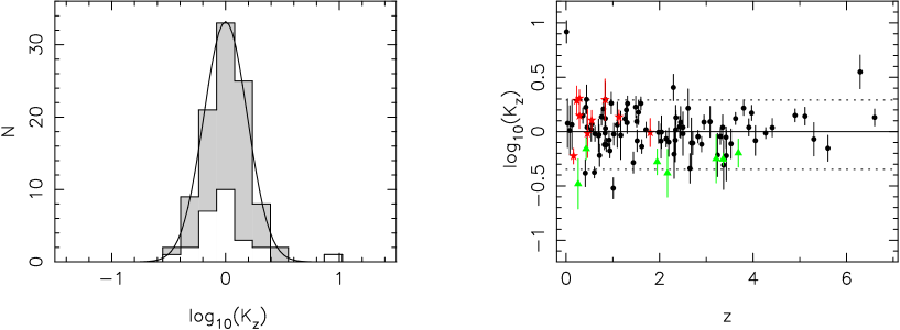
Figure 12: The distribution of the photon energy/peak luminosity ratio $K_{z}$ corresponding to the scatter about the correlation line in the right-hand panel of Figure 11. The white histogram shows the distribution of the 26 pre-Swift bursts. The curve is the best fit Gaussian distribution. The right-hand panel shows $K_{z}$ vs. redshift $z$; solid dots for long GRBs, solid stars for short GRBs, solid triangles for XRFs. The horizontal dashed lines indicate the 90% range. The objects with unusually high $K_{z}$ are GRB980425/SN1998bw at low $z$ and GRB050904 at high $z$.

This is a function of the ratio of the characteristic photon energy to the peak isotropic luminosity. The constants quoted in this definition are the mean values of the parameters so they represent the centre of the clustering of objects within the parameter space. The distribution of $K_{z}$ is plotted in Figure 12. The mean value is $\log_{10}(K_{z})=0$ or, equivalently, $K_{z}=1$. Hard-dim bursts (including most short bursts) have $K_{z}>1$, soft-bright bursts (including all XRFs) have $K_{z}<1$. The distribution is approximately log-normal (the best fit Gaussian profile is shown in Figure 12) and has a rms width of $\sigma[\log_{10}(K_{z})]=0.19$. $90\%$ of the GRBs (90 objects) are contained in the range $0.45<K_{z}<1.95$. The obvious outlier is GRB980425/SN1998bw which is either very sub-luminous or has an exceptionally high peak energy for such a dim burst. Under the hypothesis that $K_{z}$ is constant, $\chi^{2}=421$ with 99 degrees of freedom and the mean of the estimated errors on $\log{10}(K_{z})$ is 0.12 so there is clear evidence for intrinsic scatter in $K_{z}$ with an estimated $90\%$ range of $0.57<K_{z}<1.75$. The largest uncertainties arise from the estimation of $E_{wz}$ because this depends on $E_{pz}$ and the spectral indices $\beta_{X}$, $\beta_{\gamma}$. The mean value of $K_{z}$ for the pre-Swift bursts is $-0.05$ and for Swift bursts is $0.02$ so they are statistically indistinquishable. The distribution for pre-Swift bursts, plotted as the white histogram in Figure 12, sits symmetrically within the total distribution. The right-hand panel of Figure 12 shows $\log_{10}(K_{z})$ as a function of redshift, $z$. There is no obvious trend. The objects with the smallest errors that contribute most to the high $\chi^{2}$ show no dependence on redshift. Table 3 provides a complete listing of the rest frame parameters and associated errors.

6 Discussion

Within the new parameterisation of the temporal and spectral properties of the prompt GRB emission the three important quantities are the characteristic energy in the source frame, $E_{wz}$ keV (Equation 8), the energy density at the peak of the $E.F_{z}(E)$ spectrum, $Q_{pz}$ ergs kev^-1 (derived from the total fluence, Equations 2, 5 and 6) and the luminosity time, $T_{Lz}$ s, derived from the rate profile. The ratio $Q_{pz}/T_{Lz}$ gives us the peak luminosity density in ergs keV^-1 s^-1 where “peak” corresponds to both the maximum in the $E.F_{z}(E)$ spectrum and the maximum flux level in the light curve. $E_{wz}$ and $Q_{pz}/T_{Lz}$ are correlated and it is this correlation which gives rise to the Amati relation (Amati et al. 2002). The instantaneous maximum brightness of the prompt emission is characterised by a function of the photon energy/peak luminosity ratio $K_{z}$ given in Equation 15. This is not a constant but it covers a remarkably small dynamic range compared with the constituent parameters, $E_{wz}$, $Q_{pz}$ and $T_{Lz}$. Given the measurement errors it is difficult to make an accurate estimate of the intrinsic dynamic range but it is certainly less than $0.5<K_{z}<2.0$ and this holds for 100 GRBs in the sample of 101 we have analysed including long, short and XRFs, the exception being GRB980425.

6.1 Is $K_{z}$ intrinsic?

We might wonder whether the narrow range in $K_{z}$ is an artefact of the observational data or something instinsic to the nature of the GRB emission? An artificial tightness of the energy-luminosity correlation could arise in several ways; the observed quantities may be correlated by some property of the instrumentation/measurement, the measured positions of GRBs in the energy-luminosity plane could be incorrect because of some systematic error/bias or GRBs from certain areas in the plane may be selectively missed. The measured quantities in the observer frame which map to $E_{wz}$ and $Q_{pz}/T_{Lz}$ are the peak energy, $E_{p}$ keV, and the spectral energy density at the peak

$$f_{p}=\frac{N_{tot}}{T_{L}}\exp[(1-\beta_{X})(E_{p}^{-1}-1)]E_{p}^{-\beta_{X}}$$ (16)

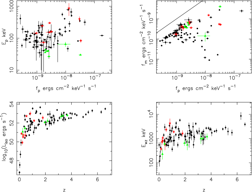
Figure 13: Top panels: Observer frame parameters $E_{p}$ and minimum observed flux density, $f_{m}$, plotted against the peak flux density, $f_{p}$. The solid line represents $f_{p}=f_{m}$. Bottom panels: Source frame parameters, peak luminosity $L_{iso}$ and characteristic energy $E_{wz}$ plotted vs. redshift $z$; solid dots for long GRBs, solid stars for short GRBs, solid triangles for XRFs.

ergs cm^-2 keV^-1 s^-1. These are plotted in the top left-hand panel of Figure 13. There is no tight clustering or significant correlation. Pearson’s correlation coefficient is $r=0.27$ and Kendall’s $\tau=0.13$, significance $2.0\sigma$. The $90\%$ range of $f_{p}$ is $4.1\times 10^{-10}-2.8\times 10^{-8}$ ergs cm^-2 keV^-1 s^-1 and the $90\%$ range of the observed peak energy is $34-412$ keV, both one to two orders of magnitude. Using the redshift to transform these into $Q_{pz}/T_{L}$ and $E_{wz}$ produces the distributions shown in Figure 10. These quantities have slightly narrower distributions in the source frame with $90\%$ ranges of $3.1\times 10^{47}-7.8\times 10^{49}$ ergs keV^-1 s^-1 and $511-3450$ keV respectively. Finally they combine in $K_{z}$ which has a rather narrow $90\%$ range of $0.45-1.95$ and some of this is attributable to the measurement errors. It is very unlikely that some systematic error or bias in the measured quantities which have a large dynamic range and are not correlated conspires to give such a tight correlation and we conclude that $K_{z}$ encodes real, useful, information about the source frame properties of the prompt emission. The rate profile fitting not only provides us with the peak flux density level but also the minumum detected flux density

$$f_{m}=N_{tot}f_{E}\exp[(1-\beta_{X})(E_{p}^{-1}-1)]E_{p}^{-\beta_{X}}$$ (17)

ergs cm^-2 keV^-1 s^-1. The top right-hand panel of Figure 13 shows $f_{m}$ vs. $f_{p}$. There is some clustering of the weaker bursts along the line $f_{p}\approx 5f_{m}$ and clearly the area above this line in the top left corner is below the threshold. It could be that we are preferentially missing hard-dim bursts while soft-dim bursts are detected but redshift works in our favour because the distant dim bursts are redshifted into the lower observation energy band where the sensitivity is higher and time dilation stretches the light curve so we have longer to detect the emission. We are undoubtedly missing low luminosity bursts especially at high redshift. The lower panels of Figure 13 shows $L_{iso}$ and $E_{wz}$ plotted vs. redshift. The hard (high $E_{wz}$) and most luminous (high $L_{iso}$) sources are seen at all redshifts while the softer, weaker sources are only seen at low redshifts, entirely as one would expect, but as we can see from Figure 12 there is no obvious difference in the distribution of $K_{z}$ as a function of $z$. There is no reason to suspect that absence of dim bursts too weak to detect is biasing the distribution in the photon energy-luminosity plane.

Our conclusions are somewhat different from Butler et al. (2007). The combination of recent Swift detections with pre-Swift results confirms the general correlation between $E_{pz}$ and $E_{iso}$ (the Amati relation) but the spread is indeed large and many bursts, including all the short bursts, are extreme outliers from the bulk correlation of the long bursts. Such a correlation is, in part, a simple consequence of the shape of a typical GRB spectrum (the Band function) but the spread and presence of many outliers renders this correlation insensitive in testing of cosmological world models. There is a clustering of events in the ratio of fluence/duration (effectively luminosity), however, we think the root of the problem is not observational bias or sensitivity thresholding but rather that the Amati relation (and similar correlations involving $E_{iso}$) are looking at the wrong parameter space. Yes, this is the demise of the existing pre-Swift high-energy correlations, but if we re-cast them in terms of the instantaneous peak luminosity and we replace $E_{pz}$ by $E_{wz}$, which combines the spectral parameters $E_{pz}$, $\beta_{X}$ and $\beta_{\gamma}$, then they reappear in a new light. The quantities in the observer frame are not correlated, the short and dim bursts are no longer outliers in the source frame correlation and there is no difference between Swift and pre-Swift detections.

6.2 Correlations involving evolution of parameters

All the analysis presented here involves average spectral and temporal properties of the prompt emission. $E_{wz}$ and $Q_{pz}$ are derived from the time-integrated spectra and $T_{Lz}$ is estimated from the full energy band light curves. We know that GRB spectra evolve with time and the light curves are different in different energy bands. In general the spectra soften as the burst proceeds, $\beta_{X}$ increases and $E_{p}$ decreases with time (e.g. Goad et al. 2007, Page et al. 2007). The light curves are shorter and more spikey at high energies than they are at low energies (Reichart et al. 2001). The lag-luminosity (Norris et al. 2000) and variability-luminosity (Reichart et al. 2001) correlations are testament to this temporal-spectral evolution. In this work we have estimated the hardness and brightness of just the peak emission. If instrumentation could follow the evolution of the characteristic energy and luminosity through the light curve each burst would form a track on the energy-luminosity density plane which may run from top right to bottom left with $K_{z}\sim constant$. The lag and variability correlations may provide a means by which scatter can be introduced in $K_{z}$ although physical reasons for this are not immediately apparent. Further analysis and better quality data are required to explore the evolution of $K_{z}$ through individual bursts.

6.3 Emission processes

The correlation between the hardness and brightness of GRB spectra, previously in the form of the Amati relation and now the correlation between $E_{wz}$ and $Q_{pz}/T_{Lz}$, is a challenge to theoretical modelling of the prompt emission. Within the standard fireball picture there are many variants involving internal and external shocks in which synchrotron emission, inverse Compton scattering and photospheric emission feature, and the fireball itself may be dominated by kinetic energy or magnetic energy (Poynting flux). The initial problem is to predict a spectrum which has the general form of the Band function with a spectral break or curvature characterised by some energy, $E_{c}$, $E_{p}$ or $E_{wz}$, and the second problem is to predict the coupling between the characteristic energy or hardness of the spectrum and the luminosity (see the review by Zhang & Mészáros 2002).

With a kinetic energy dominated outflow and a simple synchrotron model generated by internal shocks, incorporating a peak in the electron energy one expects $E_{pz}\propto\Gamma^{-2}t_{var}^{-1}L^{1/2}$ where $\Gamma$ is the bulk Lorentz factor, $t_{var}$ is the typical variability time scale associated with the internal shocks and $L$ is the luminosity (Zhang & Mészáros 2002). This is consistent with the Amati relation if $L\propto E_{iso}$ (which is not the case if we include both short and long bursts as shown above) and there is a constancy of both $\Gamma$ and $t_{var}$ across all bursts, which seems unlikely (Rees & Mészáros 2005). The relationship $E_{wz}\propto L_{iso}^{0.25}$ derived here and shown to hold for all bursts is significantly flatter than the Amati relation. If the Lorentz factor depends on luminosity, $\Gamma\propto L^{\beta}$, then we can choose $\beta\approx 1/8$ to match the observed correlation providing $t_{var}$ is independent of luminosity and approximately constant for all bursts. It is not obvious why the Lorentz factor should have such a specific and low dependence on luminosity and, again, why $t_{var}$ should be constant when the burst durations ($T_{90z}$ or $T_{Lz}$) have such a large dynamic range. Within this model the radius at which the emission occurs is given by $r\sim ct_{var}\Gamma^{2}$ so if we assume typical values of $t_{var}\sim 0.01$ s and $\Gamma\sim 300$, $r\sim 3\times 10^{13}$ cm. Furthermore, by considering the onset of X-ray afterglows observed by Swift Kumar et al. (2007) estimate that emission originates at much larger radii, between $10^{15}$ and $10^{16}$ cm, and suggest that synchrotron/inverse Compton parameters cannot account for the prompt emission.

Alternatively, we can can consider a thermal origin for the peak in the $E.F(E)$ spectrum and the correlation of the characteristic energy with luminosity, see for example Rees & Mészáros (2005), Ryde (2005) and Ghirlanda et al. (2007). If the photosphere of the expanding fireball has radius $R_{0}$, Lorentz factor $\Gamma_{0}$, a blackbody spectral component with temperature $T_{bb}$ and isotropic luminosity fraction $\varepsilon_{bb}$ of the total isotropic luminosity $L_{iso}$, then the observed temperature, $T_{obs}=(4/3)\Gamma_{0}T_{bb}$, is given by

$$\frac{T_{obs}}{1460\>{\rm keV}}=\left(\frac{\Gamma_{0}\>10^{7}\>{\rm cm}}{R_{0}}\right)^{1/2}\left(\frac{\varepsilon_{bb}L_{iso}}{10^{52}\>{\rm ergs\>s^{-1}}}\right)^{1/4}$$ (18)

Thompson (2006). This is just the Stefan-Boltzmann law modified to account for the relativistic expansion rate of the photosphere and it matches the observed correlation if $E_{wz}\propto T_{obs}$ and $\varepsilon_{bb}^{1/2}\Gamma_{0}/R_{0}$ is approximately constant for all bursts. The observed spectrum is not a single temperature blackbody. If $\varepsilon_{bb}<<1$ then any single temperature blackbody component is diluted by non-thermal (possibly power law or inverse Compton) components which combine to give the Band function. If $\varepsilon_{bb}\sim 1$ the observed spectrum must result from the summation of a large number of thermal components with a spread of temperatures that give an average of $T_{obs}$, (for example, in a manner similar to that described by Ruffini et al. 2004). We can re-arrange Equation 18 as

$$\left(\frac{\varepsilon_{bb}^{1/2}\Gamma_{0}\>10^{7}\>{\rm cm}}{R_{0}}\right)^{1/2}=\left(\frac{T_{obs}}{1460\>{\rm keV}}\right)\left(\frac{L_{iso}}{10^{52}\>{\rm ergs\>s^{-1}}}\right)^{-1/4}$$ (19)

If $T_{obs}\sim E_{wz}$ this is essentially the same as the definition of the photon energy- luminosity quasi-constant, $K_{z}$, and so, under this interpretation, the scatter in the correlation arises from variations in the fireball dimension, $R_{0}$, the Lorentz factor, $\Gamma_{0}$, or the blackbody luminosity fraction, $\varepsilon_{bb}$. If $K_{z}=1$ then we have an average fireball with $R_{0}/(\varepsilon_{bb}^{1/2}\Gamma_{0})\approx 10^{7}$ cm. If $K_{z}>1$ the fireball has a higher than average $\varepsilon_{bb}^{1/2}\Gamma_{0}$ and/or a smaller radius, $R_{0}$. If $K_{z}<1$ the fireball has a low $\varepsilon_{bb}^{1/2}\Gamma_{0}$ and/or large radius. With $\Gamma_{0}=300$ and $\varepsilon_{bb}=1$ then $R_{0}\approx 3\times 10^{9}$ cm which is the thermalization radius (i.e. the radius of the jet or fireball photosphere) estimated by Thompson, Mészáros & Rees (2007). This radius is much smaller than estimates arising from the internal shock model or recent estimates involving the onset of the X-ray afterglow (see above) so independent estimates of the radius of the prompt emission and/or the Lorentz factor may help to discriminate between thermal and internal shock models. We also note that baryonic photospheres are governed by physical argument (Mészáros et al. 2002) such that the ratio $R_{0}/\Gamma_{0}$ is constrained and the relationship between $\varepsilon_{bb}^{1/2}\Gamma_{0}/R_{0}$ and $K_{z}$ may not be as simple as we have indicated.

6.4 $K_{z}$ as a cosmological probe

The $E_{wz}-Q_{pz}/T_{Lz}$ correlation should be useful as a pseudo redshift indicator but there is evidence for intrinsic scatter in $K_{z}$, the errors in determining the characteristic energy and luminosity density are large and the correlation gradient is rather low, 0.24. In particular, reliable estimation of $E_{wz}$ requires an accurate measurement of the broadband spectrum and always involves some extrapolation to cover the source frame energy band 1-10000 keV. Without a good measurement of the peak energy, $E_{p}$, we can’t calculate a good estimate of $Q_{pz}$ from $Q_{z}$. The launch of GLAST in the near future will hopefully provide excellent high-energy spectral measurements which will tie down the spectral parameters more precisely. The intrinsic scatter may arise in several ways. If the dominant emission mechanism is non-thermal then the coupling of the Lorentz factor of the expansion with the luminosity and the variability time associated with the internal shocks may be the root cause. If thermal processes dominate then the ratio $R_{0}/\Gamma_{0}$ may vary as discussed above. Because we can identify classes which fall predominately at $K_{z}>1$ (shorts) and $K_{z}<1$ (XRFs) there is some hope that additional parameters which distinguish these classes may serve to narrow the distribution. In the above discussion we made no mention of collimation or beaming of the outflow. Since the Amati relation involving $E_{iso}$ has been transformed into the present universal correlation involving $L_{iso}$ the simple beaming argument that underpinned the Ghirlanda relation (Ghirlanda et al. 2004) is not directly applicable and currently there is no simple physical model which links collimation to scatter in peak luminosity or the characteristic photon energy. However, it is not unreasonable to suppose that collimation may introduce scatter in the peak luminosity, and that correlation of $K_{z}$ with afterglow parameters such as optical jet break times $t_{break}$ or the time of the start of the final X-ray afterglow, $T_{a}$ (Willingale et al. 2007), may be fruitful. In its present form $K_{z}$ is not a sensitive cosmological probe but the signs are that it may be in the future.

7 Conclusion

The equivalent isotropic energy, $E_{iso}$ ergs, of a GRB can be expressed as the product of two source frame terms, a characteristic photon energy, $E_{wz}$ keV, calculated from the shape of the spectrum across the range 1-10000 keV and the energy density at the peak of the $E.F_{z}(E)$ spectrum, $Q_{pz}$ ergs keV^-1. The correlation trend between $E_{wz}$ and $Q_{pz}$ gives rise to the Amati relation. By stacking the samples of a GRB light curve into descending order we can construct a rate profile. The functional form of such rate profiles is common to the vast majority of bursts. Fitting the profile gives us a luminosity time, $T_{Lz}$ s, a measure of the burst duration which can be used to convert the energy density at the peak to a luminosity density at peak, $Q_{pz}/T_{Lz}$ ergs keV^-1 s^-1. We can calculate the peak equivalent isotropic luminosity as a product $L_{iso}=E_{wz}Q_{pz}/T_{Lz}=E_{iso}/T_{Lz}$ ergs s^-1.

$E_{wz}$ is a characteristic photon energy or a measure of the colour or hardness of the burst and $Q_{pz}/T_{Lz}$ is a measure of the instantaneous peak brightness. We have gathered and analysed sufficient spectral and temporal data from 101 bursts to produce the relation between $E_{wz}$ vs. $Q_{pz}/T_{Lz}$ and $E_{wz}$ vs. $L_{iso}$, shown in Figure 11, which constitutes the closest thing we have to an intrinsic colour-magnitude diagram for the peak emission from GRBs, $E_{wz}\propto L_{iso}^{0.25}$. All bursts are clustered such that we can construct a intrinsic colour-magnitude quasi constant $K_{z}$, which is a function of the source frame characteristic photon energy/peak luminosity ratio given by Equation 15. The range of equivalent isotropic energy that drives the expanding fireball is very large, 6 orders of magnitude (Figure 3), but the instantaneous hardness/brightness of the peak emission covers a very small intrinsic dynamic range, $\approx 4$.

The existence and form of $K_{z}$ indicates that the physical mechanism for the Gamma-ray production at the photosphere of the fireball is common to all bursts and is probably thermal although many other possibilities are not ruled out. If the prompt spectra are dominated by thermal photons the scatter in $K_{z}$ may be attributed to variations in the size and/or Lorentz factor of the fireball. XRFs have low $\Gamma_{0}$ and/or large radii. Short bursts have high $\Gamma_{0}$ and/or small radii. The relation between $T_{Lz}$ vs. $Q_{pz}$ clearly separates short from long, but both classes have the same instantaneous peak hardness/brightness.

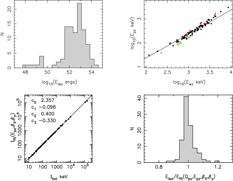
Figure 3: Top panels: The distribution of $E_{iso}$ and the correlation of $E_{pz}$ vs. $E_{wz}$ for GRBs listed in Table 1; solid dots for long GRBs, solid stars for short GRBs, solid triangles for XRFs. The solid line is $E_{pz}=0.23E_{wz}$ rather than the best fit correlation which is a little steeper (see text). Bottom panels: Comparison of the functional fit to the bolometric integral $I_{fit}$ and the value calculated by numerical integration of the Band function over the interval 1-10000 keV for the GRBs in Table 1. The right-hand panel shows the distribution of the ratio of $E_{iso}$ to the value obtained using $I_{fit}$.

Figure 5: The rate profile function, Equation 12.

Figure 7: Left-hand panel: The distribution of luminosity times, $T_{L}$ s, and the $\Sigma$ statistic from the fit. Right-hand panel: The correlation between rate profile index $C_{L}$ and the ratio of $T_{45}$ derived directly from the data and $T_{L}$ derived from the profile function fit.

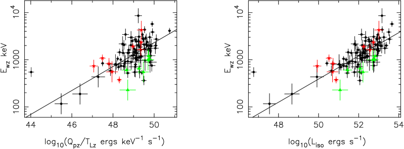
Figure 11: Left-hand panel: The correlation between characteristic energy $E_{wz}$ keV and the peak luminosity density $Q_{pz}/T_{Lz}$ ergs keV^-1 s^-1. Right-hand panel: $E_{wz}$ keV vs. the peak isotropic luminosity, $L_{iso}=E_{wz}Q_{pz}/T_{Lz}$ ergs s^-1. In both plots solid dots for long GRBs, solid stars for short GRBs, solid triangles for XRFs. The object with the largest $E_{wz}$, 8600 keV, is GRB050904.

Table 1: Observed spectral parameters; $\beta_{X}$, low spectral index, $E_{p}$, peak energy keV (if no error quoted then calculated assuming fixed $E_{cut}$, $E_{p}=(1-\beta_{X})*150$ keV), $\beta_{\gamma}$, high spectral index (if no error quoted then fixed at average of 1.3), $F_{tot}$, fluence ergs cm^-2, $E_{1}$ to $E_{2}$, observed energy band keV. References: (0) Swift BAT ibid., (1) Golenetskii et al., 2005, (2) Villasenor et al., 2005, (3) Barthelmy et al. 2005, Amati et al. 2006, Campana et al. 2006, (4) Golenetskii et al., 2005, (5) Golenetskii et al. 2005, Burrows D.N. et al. 2006, (6) Romano et al., 2006, (7) Amati et al. 2007, Montanari & Pian 2007, (8) Amati et al. 2007, Golenetskii et al. 2006, (9) Page et al. 2007, (10) Ghirlanda et al. 2004, (11) Friedman & Bloom 2005, (12) Sakamoto et al. 2005, (13) Atteia et al. 2005, (14) Piro et al. 2005, Amati 2007, (15) Galassi et al. 2004, Amati 2007, (16) Schaefer 2007, Firmani et al. 2006. (17) Golenetskii et al. 2007.

GRB	$\beta_{X}$	$E_{p}$	$\beta_{\gamma}$	$F_{tot}$	$E_{1}$	$E_{2}$	refs
970228	$0.54\pm 0.08$	$115\pm 38$	$1.50\pm 0.40$	$(11.0\pm 1.0)10^{-6}$	40	700	10
970508	$0.71\pm 0.10$	$79\pm 23$	$1.20\pm 0.25$	$(1.8\pm 0.3)10^{-6}$	40	700	10
971214	$-0.24\pm 0.10$	$155\pm 30$	$1.70\pm 1.10$	$(8.8\pm 0.9)10^{-6}$	40	700	10
980425	$0.27\pm 0.13$	$118\pm 24$	$1.30$	$(3.8\pm 0.4)10^{-6}$	20	2000	10
980613	$0.43\pm 0.20$	$93\pm 43$	$1.70\pm 0.60$	$(1.0\pm 0.2)10^{-6}$	40	700	10
980703	$0.31\pm 0.14$	$255\pm 51$	$1.39\pm 0.14$	$(23.0\pm 0.2)10^{-6}$	20	2000	10
990123	$-0.11\pm 0.08$	$781\pm 62$	$1.45\pm 0.97$	$(3.0\pm 0.4)10^{-4}$	40	700	10
990506	$0.37\pm 0.15$	$283\pm 57$	$1.15\pm 0.38$	$(1.9\pm 0.2)10^{-4}$	20	2000	10
990510	$0.23\pm 0.05$	$163\pm 16$	$1.70\pm 0.40$	$(1.9\pm 0.2)10^{-5}$	40	700	10
990705	$0.05\pm 0.20$	$189\pm 15$	$1.20\pm 0.10$	$(7.5\pm 0.8)10^{-5}$	40	700	10
990712	$0.88\pm 0.07$	$65\pm 11$	$1.48\pm 0.56$	$(0.6\pm 0.3)10^{-5}$	40	700	10
991216	$0.23\pm 0.13$	$318\pm 64$	$1.18\pm 0.39$	$(1.9\pm 0.2)10^{-4}$	20	2000	10
010921	$0.49\pm 0.16$	$106\pm 21$	$1.30$	$(10.0\pm 1.0)10^{-6}$	30	700	10
011121	$0.42\pm 0.14$	$217\pm 26$	$1.30$	$(96.6\pm 1.0)10^{-6}$	40	700	14
011211	$-0.16\pm 0.09$	$59\pm 8$	$1.30$	$(5.1\pm 0.2)10^{-6}$	40	700	14
021004	$0.01\pm 0.19$	$80\pm 35$	$1.30\pm 0.46$	$(2.6\pm 0.6)10^{-6}$	2	400	11
021211	$-0.15\pm 0.09$	$47\pm 9$	$1.37\pm 0.42$	$(2.2\pm 0.2)10^{-6}$	30	400	10
030115A	$0.28\pm 0.14$	$83\pm 37$	$1.20\pm 0.40$	$(2.3\pm 0.3)10^{-6}$	2	400	16
030226	$-0.05\pm 0.10$	$108\pm 22$	$1.30$	$(6.4\pm 0.6)10^{-6}$	30	400	10
030323	$-0.20\pm 0.20$	$53\pm 30$	$1.30$	$(1.2\pm 0.3)10^{-6}$	2	400	13
030328	$0.00\pm 0.11$	$110\pm 22$	$1.30$	$(2.6\pm 0.2)10^{-5}$	30	400	10
030429	$0.10\pm 0.20$	$35\pm 10$	$1.30$	$(0.8\pm 0.1)10^{-6}$	2	400	12
040924	$0.17\pm 0.05$	$125\pm 12$	$1.30$	$(2.7\pm 0.1)10^{-6}$	20	500	16
041006	$0.37\pm 0.10$	$63\pm 13$	$1.30$	$(7.0\pm 0.5)10^{-6}$	30	400	15
050126	$0.06\pm 0.20$	$158\pm 20$	$1.30$	$(8.4\pm 0.8)10^{-7}$	15	150	0
050315	$0.76\pm 0.06$	$36$	$1.30$	$(3.2\pm 0.1)10^{-6}$	15	150	0
050318	$0.34\pm 0.20$	$47\pm 9$	$1.30$	$(10.8\pm 0.8)10^{-7}$	15	150	0
050319	$0.66\pm 0.15$	$51$	$1.30$	$(1.3\pm 0.1)10^{-6}$	15	150	0
050401	$0.11\pm 0.07$	$132\pm 16$	$1.30$	$(8.2\pm 0.3)10^{-6}$	15	150	0
050505	$-0.01\pm 0.20$	$102\pm 0$	$1.30$	$(2.5\pm 0.2)10^{-6}$	15	150	0
050509B	$0.04\pm 0.20$	$144$	$1.30$	$(0.9\pm 0.2)10^{-8}$	15	150	0
050525A	$-0.13\pm 0.07$	$82\pm 4$	$1.30$	$(15.3\pm 0.2)10^{-6}$	15	150	0
050603	$-0.19\pm 0.04$	$349\pm 28$	$1.30$	$(6.4\pm 0.2)10^{-6}$	15	150	1
050709	$-0.47\pm 0.13$	$83\pm 10$	$1.30$	$(4.0\pm 0.4)10^{-7}$	2	400	2
050724	$0.80\pm 0.17$	$30$	$1.30$	$(1.0\pm 0.1)10^{-6}$	15	150	3
050730	$0.15\pm 0.10$	$127$	$1.30$	$(2.4\pm 0.2)10^{-6}$	15	150	0
050802	$0.15\pm 0.10$	$127$	$1.30$	$(2.0\pm 0.2)10^{-6}$	15	150	0
050803	$0.05\pm 0.08$	$142$	$1.30$	$(2.2\pm 0.1)10^{-6}$	15	150	0
050813	$-0.02\pm 0.20$	$153$	$1.30$	$(0.4\pm 0.1)10^{-7}$	15	150	0
050814	$0.61\pm 0.13$	$58$	$1.30$	$(2.0\pm 0.2)10^{-6}$	15	150	0
050820A	$-0.03\pm 0.09$	$246\pm 96$	$1.30$	$(3.4\pm 0.2)10^{-6}$	15	150	0
050904	$0.07\pm 0.14$	$413\pm 140$	$1.30$	$(4.8\pm 0.2)10^{-6}$	15	150	0
050908	$0.50\pm 0.12$	$75$	$1.30$	$(4.8\pm 0.5)10^{-7}$	15	150	0
050922C	$0.04\pm 0.05$	$130\pm 37$	$1.30$	$(16.2\pm 0.5)10^{-7}$	15	150	0
051022	$0.18\pm 0.04$	$510\pm 35$	$1.30$	$(26.1\pm 0.9)10^{-5}$	20	2000	4
051109A	$0.23\pm 0.15$	$157\pm 111$	$1.30$	$(2.2\pm 0.3)10^{-6}$	15	150	4
051109B	$-0.11\pm 0.20$	$41\pm 32$	$1.30$	$(2.6\pm 0.4)10^{-7}$	15	150	0
051111	$0.04\pm 0.05$	$211\pm 50$	$1.30$	$(4.1\pm 0.1)10^{-6}$	15	150	0
051221A	$0.08\pm 0.04$	$402\pm 72$	$1.30$	$(11.5\pm 0.3)10^{-7}$	15	150	5
060108	$0.65\pm 0.12$	$52$	$1.30$	$(3.7\pm 0.4)10^{-7}$	15	150	0
060115	$0.09\pm 0.20$	$62\pm 18$	$1.30$	$(1.7\pm 0.2)10^{-6}$	15	150	0
060116	$-0.01\pm 0.14$	$151$	$1.30$	$(2.4\pm 0.3)10^{-6}$	15	150	0
060124	$0.66\pm 0.17$	$193\pm 49$	$1.30$	$(4.6\pm 0.5)10^{-7}$	15	150	6
060206	$0.38\pm 0.19$	$75\pm 22$	$1.30$	$(8.3\pm 0.4)10^{-7}$	15	150	0
060210	$0.18\pm 0.12$	$123$	$1.30$	$(7.7\pm 0.4)10^{-6}$	15	150	0
060218	$-0.76\pm 0.20$	$30\pm 20$	$1.30$	$(1.6\pm 0.2)10^{-6}$	15	150	7
060223A	$0.44\pm 0.09$	$83$	$1.30$	$(6.7\pm 0.5)10^{-7}$	15	150	0
060418	$0.38\pm 0.04$	$230\pm 46$	$1.30$	$(8.3\pm 0.3)10^{-6}$	15	150	0
060502A	$0.07\pm 0.05$	$139$	$1.30$	$(2.3\pm 0.1)10^{-6}$	15	150	0
060502B	$-0.08\pm 0.20$	$162$	$1.30$	$(4.0\pm 0.5)10^{-8}$	15	150	0
060510B	$0.48\pm 0.20$	$89\pm 6$	$1.30$	$(4.1\pm 0.2)10^{-6}$	15	150	0
060522	$0.21\pm 0.12$	$118$	$1.30$	$(1.1\pm 0.1)10^{-6}$	15	150	0
060526	$0.74\pm 0.16$	$39$	$1.30$	$(1.3\pm 0.2)10^{-6}$	15	150	0
060604	$0.59\pm 0.20$	$61$	$1.30$	$(0.4\pm 0.1)10^{-6}$	15	150	0
060605	$-0.07\pm 0.11$	$160$	$1.30$	$(7.0\pm 0.9)10^{-7}$	15	150	0
060607A	$0.05\pm 0.20$	$131\pm 40$	$1.30$	$(2.6\pm 0.1)10^{-6}$	15	150	0
060614	$0.66\pm 0.03$	$68\pm 50$	$1.30$	$(20.4\pm 0.4)10^{-6}$	15	150	8
060707	$-0.42\pm 0.20$	$60\pm 53$	$1.30$	$(1.6\pm 0.2)10^{-6}$	15	150	0
060714	$0.64\pm 0.08$	$54$	$1.30$	$(2.8\pm 0.2)10^{-6}$	15	150	0
060729	$0.51\pm 0.11$	$73$	$1.30$	$(2.6\pm 0.2)10^{-6}$	15	150	0
060801	$-0.99\pm 0.19$	$298$	$1.30$	$(8.0\pm 1.0)10^{-8}$	15	150	0
060814	$0.43\pm 0.16$	$257\pm 90$	$1.30$	$(14.6\pm 0.2)10^{-6}$	15	150	0
060904B	$0.40\pm 0.11$	$90$	$1.30$	$(1.6\pm 0.1)10^{-6}$	15	150	0
060906	$0.71\pm 0.08$	$43$	$1.30$	$(2.2\pm 0.1)10^{-6}$	15	150	0
060908	$-0.15\pm 0.16$	$153\pm 29$	$1.30$	$(2.8\pm 0.1)10^{-6}$	15	150	0
060912	$0.45\pm 0.06$	$82$	$1.30$	$(13.5\pm 0.6)10^{-7}$	15	150	0
060927	$-0.07\pm 0.20$	$72\pm 18$	$1.30$	$(11.3\pm 0.7)10^{-7}$	15	150	0
061004	$0.46\pm 0.07$	$80$	$1.30$	$(5.7\pm 0.3)10^{-7}$	15	150	0
061006	$-0.38\pm 0.20$	$664\pm 186$	$1.30$	$(1.4\pm 0.1)10^{-6}$	15	150	17
061007	$-0.38\pm 0.02$	$407\pm 19$	$1.30$	$(44.4\pm 0.6)10^{-6}$	15	150	0
061110A	$0.35\pm 0.09$	$97$	$1.30$	$(10.6\pm 0.8)10^{-7}$	15	150	0
061121	$0.05\pm 0.02$	$557\pm 66$	$1.30$	$(13.7\pm 0.2)10^{-6}$	15	150	9
061201	$-0.67\pm 0.15$	$873\pm 371$	$1.30$	$(3.3\pm 0.3)10^{-7}$	15	150	0
061210	$0.19\pm 0.20$	$121$	$1.30$	$(1.1\pm 0.2)10^{-6}$	15	150	0
061217	$-0.62\pm 0.20$	$243$	$1.30$	$(4.2\pm 0.7)10^{-8}$	15	150	0
061222B	$0.71\pm 0.20$	$40\pm 2$	$1.30$	$(2.2\pm 0.2)10^{-6}$	15	150	0
070110	$0.24\pm 0.08$	$114$	$1.30$	$(1.6\pm 0.1)10^{-6}$	15	150	0
070208	$0.50\pm 0.20$	$75$	$1.30$	$(0.4\pm 0.1)10^{-6}$	15	150	0
070318	$0.07\pm 0.06$	$139$	$1.30$	$(2.5\pm 0.1)10^{-6}$	15	150	0
070411	$0.35\pm 0.07$	$97$	$1.30$	$(2.7\pm 0.2)10^{-6}$	15	150	0
070506	$-0.11\pm 0.20$	$53\pm 33$	$1.30$	$(2.1\pm 0.2)10^{-7}$	15	150	0
070508	$-0.13\pm 0.02$	$169$	$1.30$	$(19.6\pm 0.3)10^{-6}$	15	150	0
070521	$-0.11\pm 0.03$	$166$	$1.30$	$(8.0\pm 0.2)10^{-6}$	15	150	0
070529	$0.11\pm 0.12$	$133$	$1.30$	$(2.6\pm 0.2)10^{-6}$	15	150	0
070611	$0.44\pm 0.18$	$83$	$1.30$	$(3.9\pm 0.6)10^{-7}$	15	150	0
070612A	$0.41\pm 0.07$	$88$	$1.30$	$(10.6\pm 0.6)10^{-6}$	15	150	0
070714B	$0.04\pm 0.15$	$144$	$1.30$	$(6.4\pm 0.9)10^{-7}$	15	150	0
070721B	$-0.14\pm 0.08$	$171$	$1.30$	$(3.0\pm 0.2)10^{-6}$	15	150	0
070724A	$0.51\pm 0.20$	$73$	$1.30$	$(2.8\pm 0.7)10^{-8}$	15	150	0
070802	$0.42\pm 0.18$	$87$	$1.30$	$(2.5\pm 0.5)10^{-7}$	15	150	0
070810A	$0.82\pm 0.10$	$26$	$1.30$	$(6.1\pm 0.7)10^{-7}$	15	150	0

Table 2: Observed temporal parameters; $T_{90}$ secs, luminosity time $T_{L}$ secs, luminosity index $C_{L}$ , luminosity profile fitting statistic $\Sigma$. Errors were estimated by assuming $\Sigma$ was distributed as $\chi^{2}$.

GRB	instr	class	$T_{90}$	$T_{L}$	$C_{L}$	$\Sigma$
970228	SAX	Long	80.0	$9.7\pm 0.6$	$2.41\pm 0.07$	1.55
970508	SAX	Long	20.0	$4.2\pm 0.1$	$2.01\pm 0.03$	1.55
971214	SAX	Long	35.0	$10.6\pm 0.2$	$1.52\pm 0.02$	1.31
980425	SAX	Long	37.4	$16.\pm 1.$	$1.54\pm 0.13$	0.94
980613	BATSE	Long	20.0	$12.\pm 1.$	$1.32\pm 0.21$	1.19
980703	BATSE	Long	102	$20.0\pm 0.4$	$1.56\pm 0.03$	0.30
990123	SAX	Long	100.0	$22.7\pm 0.2$	$1.94\pm 0.01$	1.37
990506	BATSE	Long	220	$14.00\pm 0.10$	$2.35\pm 0.01$	1.83
990510	SAX	Long	75.0	$5.23\pm 0.06$	$2.48\pm 0.01$	1.23
990705	SAX	Long	42.0	$26.8\pm 0.9$	$1.64\pm 0.03$	6.51
990712	SAX	XRF	20.0	$4.1\pm 0.3$	$2.80\pm 0.08$	4.67
991216	BATSE	Long	24.9	$3.89\pm 0.04$	$2.59\pm 0.01$	4.59
010921	HETE-2	Long	24.6	$12.3\pm 0.4$	$1.26\pm 0.05$	0.35
011121	SAX	Long	37.0	$18.9\pm 0.6$	$2.14\pm 0.04$	3.10
011211	SAX	Long	270	$133.\pm 5.$	$1.26\pm 0.06$	0.99
021004	HETE-2	Long	49.7	$11.4\pm 0.7$	$1.62\pm 0.10$	0.39
021211	HETE-2	Long	2.4	$2.0\pm 0.2$	$1.28\pm 0.09$	0.44
030115A	HETE-2	Long	36.0	$8.4\pm 0.4$	$1.73\pm 0.08$	0.28
030226	HETE-2	Long	76.8	$27.3\pm 0.9$	$1.60\pm 0.06$	0.32
030323	HETE-2	Long	19.6	$2.9\pm 0.8$	$1.36\pm 0.28$	0.20
030328	HETE-2	Long	140	$45.8\pm 0.7$	$1.66\pm 0.02$	0.27
030429	HETE-2	Long	24.6	$5.8\pm 0.7$	$2.13\pm 0.19$	0.94
040924	HETE-2	Long	5.0	$1.13\pm 0.07$	$2.05\pm 0.08$	3.40
041006	HETE-2	Long	24.6	$13.1\pm 0.4$	$1.37\pm 0.04$	1.63
050126	Swift	Long	25.7	$7.7\pm 0.4$	$1.65\pm 0.09$	0.39
050315	Swift	XRF	96.0	$21.6\pm 0.5$	$1.62\pm 0.04$	0.14
050318	Swift	Long	31.3	$5.3\pm 0.3$	$1.40\pm 0.09$	1.11
050319	Swift	Long	149	$4.0\pm 0.3$	$1.93\pm 0.11$	0.68
050401	Swift	Long	33.3	$6.1\pm 0.2$	$1.78\pm 0.05$	0.19
050505	Swift	Long	63.0	$11.4\pm 0.4$	$1.50\pm 0.08$	0.19
050509B	Swift	Short	0.07	$0.043\pm 0.005$	$1.61\pm 0.20$	0.47
050525A	Swift	Long	8.8	$3.9\pm 0.1$	$1.58\pm 0.03$	1.45
050603	Swift	Long	13.0	$0.84\pm 0.02$	$2.74\pm 0.03$	0.38
050709	HETE-2	Short	0.22	$0.056\pm 0.004$	$2.26\pm 0.08$	3.19
050724	Swift	XRF	152	$0.48\pm 0.02$	$3.17\pm 0.06$	0.32
050730	Swift	Long	155	$25.8\pm 0.8$	$1.81\pm 0.06$	0.25
050802	Swift	Long	30.9	$6.1\pm 0.3$	$1.59\pm 0.09$	0.22
050803	Swift	Long	89.0	$14.3\pm 0.5$	$1.85\pm 0.05$	0.12
050813	Swift	Short	0.45	$0.073\pm 0.009$	$1.71\pm 0.23$	0.49
050814	Swift	Long	144	$11.1\pm 0.6$	$1.74\pm 0.11$	0.12
050820A	Swift	Long	240	$11.6\pm 0.2$	$1.75\pm 0.03$	0.16
050904	Swift	Long	173	$57.\pm 1.$	$1.62\pm 0.04$	0.28
050908	Swift	Long	20.3	$5.5\pm 0.3$	$1.45\pm 0.09$	0.15
050922C	Swift	Long	4.1	$1.81\pm 0.07$	$1.65\pm 0.05$	0.89
051022	Konus	Long	197	$10.9\pm 0.3$	$1.81\pm 0.04$	4.91
051109A	Swift	Long	37.0	$2.9\pm 0.2$	$2.00\pm 0.13$	0.28
051109B	Swift	Long	15.0	$1.9\pm 0.2$	$1.79\pm 0.16$	0.31
051111	Swift	Long	42.6	$13.4\pm 0.3$	$1.66\pm 0.04$	0.11
051221A	Swift	Short	1.40	$0.118\pm 0.003$	$2.85\pm 0.03$	3.22
060108	Swift	Long	14.4	$4.4\pm 0.3$	$1.46\pm 0.11$	0.22
060115	Swift	Long	141	$17.5\pm 0.6$	$1.78\pm 0.06$	0.35
060116	Swift	Long	105	$9.1\pm 0.5$	$1.57\pm 0.12$	0.15
060124	Swift	Long	321	$4.1\pm 0.3$	$1.58\pm 0.13$	0.41
060206	Swift	Long	7.7	$3.3\pm 0.1$	$1.42\pm 0.05$	0.22
060210	Swift	Long	220	$24.9\pm 0.6$	$1.92\pm 0.04$	0.61
060218	Swift	Long	2100	$20.4\pm 0.9$	$1.82\pm 0.09$	0.12
060223A	Swift	Long	11.4	$4.7\pm 0.3$	$1.36\pm 0.10$	0.14
060418	Swift	Long	95.8	$16.5\pm 0.3$	$1.93\pm 0.02$	1.05
060502A	Swift	Long	32.0	$12.0\pm 0.4$	$1.38\pm 0.06$	0.77
060502B	Swift	Short	0.13	$0.058\pm 0.006$	$2.41\pm 0.13$	0.60
060510B	Swift	Long	276	$57.\pm 1.$	$1.65\pm 0.04$	0.24
060522	Swift	Long	69.3	$9.1\pm 0.4$	$1.77\pm 0.09$	0.10
060526	Swift	XRF	298	$6.7\pm 0.3$	$2.39\pm 0.07$	0.72
060604	Swift	Long	7.8	$2.3\pm 0.2$	$1.49\pm 0.24$	0.14
060605	Swift	Long	14.8	$7.9\pm 0.4$	$1.46\pm 0.09$	0.15
060607A	Swift	Long	100	$15.2\pm 0.4$	$1.88\pm 0.04$	0.18
060614	Swift	Long	108	$26.7\pm 0.4$	$2.13\pm 0.02$	4.70
060707	Swift	Long	66.2	$10.0\pm 0.5$	$1.72\pm 0.09$	0.11
060714	Swift	Long	115	$23.0\pm 0.6$	$1.62\pm 0.05$	0.20
060729	Swift	Long	112	$17.2\pm 0.5$	$1.59\pm 0.05$	0.44
060801	Swift	Short	0.49	$0.20\pm 0.01$	$1.70\pm 0.11$	0.51
060814	Swift	Long	128	$25.5\pm 0.3$	$2.17\pm 0.01$	1.25
060904B	Swift	Long	190	$4.9\pm 0.2$	$2.17\pm 0.04$	0.53
060906	Swift	XRF	43.5	$12.1\pm 0.4$	$1.67\pm 0.07$	0.61
060908	Swift	Long	19.0	$9.1\pm 0.3$	$1.09\pm 0.06$	0.31
060912	Swift	Long	6.0	$1.53\pm 0.06$	$2.02\pm 0.05$	1.57
060927	Swift	Long	10.0	$3.9\pm 0.1$	$1.92\pm 0.05$	0.44
061004	Swift	Long	6.2	$2.4\pm 0.1$	$1.89\pm 0.07$	0.28
061006	Swift	Long	129	$0.47\pm 0.01$	$3.12\pm 0.03$	1.26
061007	Swift	Long	74.2	$23.2\pm 0.2$	$1.90\pm 0.01$	5.04
061110A	Swift	Long	44.6	$13.4\pm 0.5$	$1.57\pm 0.07$	0.33
061121	Swift	Long	81.3	$5.34\pm 0.06$	$2.58\pm 0.01$	1.28
061201	Swift	Short	0.76	$0.22\pm 0.01$	$1.96\pm 0.07$	0.55
061210	Swift	Long	85.3	$0.030\pm 0.001$	$4.29\pm 0.04$	13.4
061217	Swift	Short	0.21	$0.15\pm 0.01$	$1.76\pm 0.16$	0.08
061222B	Swift	XRF	40.0	$10.7\pm 0.5$	$1.70\pm 0.08$	0.43
070110	Swift	Long	87.3	$18.1\pm 0.6$	$1.63\pm 0.07$	0.25
070208	Swift	Long	47.7	$2.9\pm 0.3$	$1.69\pm 0.17$	1.12
070318	Swift	Long	119	$12.7\pm 0.3$	$1.91\pm 0.04$	0.14
070411	Swift	Long	116	$27.0\pm 0.8$	$1.66\pm 0.05$	0.26
070506	Swift	Long	4.3	$2.1\pm 0.1$	$1.39\pm 0.12$	0.55
070508	Swift	Long	20.8	$6.59\pm 0.09$	$2.07\pm 0.02$	1.30
070521	Swift	Long	38.4	$12.2\pm 0.2$	$1.69\pm 0.03$	0.42
070529	Swift	Long	108	$8.5\pm 0.4$	$1.90\pm 0.09$	0.29
070611	Swift	Long	13.2	$2.6\pm 0.2$	$1.67\pm 0.18$	0.28
070612A	Swift	Long	359	$32.4\pm 0.9$	$1.91\pm 0.05$	0.27
070714B	Swift	Long	63.9	$0.48\pm 0.02$	$2.87\pm 0.07$	0.55
070721B	Swift	Long	345	$12.5\pm 0.4$	$1.87\pm 0.05$	0.40
070724A	Swift	Short	0.40	$0.11\pm 0.01$	$1.75\pm 0.16$	0.66
070802	Swift	Long	16.9	$3.5\pm 0.3$	$1.74\pm 0.15$	0.27
070810A	Swift	XRF	10.9	$4.1\pm 0.2$	$1.18\pm 0.10$	0.46

Table 3: Source frame parameters; $z$ redshift, values from tabulations in Amati (2006), Ghirlanda et al. (2004) and http://swift.gsfc.nasa.gov/docs/swift/archive/grb_table/. References for all the Swift redshifts are provided on this WWW data table. $E_{wz}$ keV, $Q_{pz}$ ergs keV^-1, $T_{Lz}$ secs, photon energy/peak luminosity ratio $K_{z}$.

GRB	$z$	$E_{wz}$	$Q_{pz}$	$T_{Lz}$	$K_{z}$
970228	0.695	$927\pm 320$	$(0.3\pm 0.1)10^{50}$	$5.7\pm 0.3$	$1.21\pm 0.96$
970508	0.835	$906\pm 279$	$(0.9\pm 0.3)10^{49}$	$2.30\pm 0.06$	$1.16\pm 0.83$
971214	3.420	$1981\pm 431$	$(1.5\pm 0.4)10^{50}$	$2.41\pm 0.04$	$1.00\pm 0.51$
980425	0.009	$550\pm 124$	$(1.7\pm 0.5)10^{45}$	$16.\pm 1.$	$0.18\pm 0.10$
980613	1.096	$807\pm 382$	$(0.7\pm 0.4)10^{49}$	$5.7\pm 0.7$	$1.02\pm 1.12$
980703	0.966	$2061\pm 460$	$(3.4\pm 0.9)10^{49}$	$10.2\pm 0.2$	$0.50\pm 0.26$
990123	1.600	$5736\pm 732$	$(7.0\pm 1.4)10^{50}$	$8.72\pm 0.09$	$0.37\pm 0.11$
990506	1.307	$3000\pm 674$	$(3.7\pm 1.1)10^{50}$	$6.07\pm 0.04$	$0.66\pm 0.35$
990510	1.619	$1539\pm 215$	$(1.3\pm 0.2)10^{50}$	$2.00\pm 0.02$	$1.29\pm 0.42$
990705	0.843	$1484\pm 189$	$(1.7\pm 0.4)10^{50}$	$14.5\pm 0.5$	$0.91\pm 0.29$
990712	0.430	$605\pm 119$	$(1.3\pm 0.7)10^{49}$	$2.9\pm 0.2$	$1.78\pm 0.91$
991216	1.020	$2732\pm 614$	$(2.4\pm 0.7)10^{50}$	$1.92\pm 0.02$	$0.85\pm 0.45$
010921	0.450	$781\pm 173$	$(1.2\pm 0.4)10^{49}$	$8.5\pm 0.3$	$1.08\pm 0.56$
011121	0.360	$1395\pm 217$	$(4.3\pm 0.9)10^{49}$	$13.9\pm 0.5$	$0.72\pm 0.27$
011211	2.140	$733\pm 123$	$(1.4\pm 0.3)10^{50}$	$43.\pm 2.$	$1.38\pm 0.54$
021004	2.335	$1072\pm 481$	$(0.4\pm 0.2)10^{50}$	$3.4\pm 0.2$	$1.27\pm 1.32$
021211	1.010	$367\pm 79$	$(3.1\pm 0.8)10^{49}$	$1.0\pm 0.1$	$4.43\pm 2.24$
030115A	2.500	$1368\pm 625$	$(0.3\pm 0.2)10^{50}$	$2.4\pm 0.1$	$1.04\pm 1.10$
030226	1.980	$1249\pm 283$	$(0.9\pm 0.2)10^{50}$	$9.2\pm 0.3$	$1.04\pm 0.55$
030323	3.370	$891\pm 445$	$(0.4\pm 0.3)10^{50}$	$0.7\pm 0.2$	$2.17\pm 2.50$
030328	1.520	$1106\pm 247$	$(2.6\pm 0.7)10^{50}$	$18.2\pm 0.3$	$1.27\pm 0.66$
030429	2.650	$555\pm 168$	$(0.3\pm 0.1)10^{50}$	$1.6\pm 0.2$	$2.67\pm 1.90$
040924	0.859	$995\pm 137$	$(0.9\pm 0.1)10^{49}$	$0.61\pm 0.04$	$1.42\pm 0.46$
041006	0.716	$524\pm 120$	$(0.4\pm 0.1)10^{50}$	$7.6\pm 0.2$	$2.11\pm 1.12$
050126	1.290	$1444\pm 237$	$(0.7\pm 0.2)10^{49}$	$3.3\pm 0.2$	$0.64\pm 0.25$
050315	1.949	$652\pm 175$	$(1.3\pm 0.4)10^{50}$	$7.3\pm 0.2$	$2.25\pm 1.40$
050318	1.440	$547\pm 118$	$(2.5\pm 0.7)10^{49}$	$2.2\pm 0.1$	$2.40\pm 1.22$
050319	3.240	$1221\pm 552$	$(0.6\pm 0.3)10^{50}$	$0.94\pm 0.06$	$1.63\pm 1.71$
050401	2.900	$2008\pm 315$	$(1.9\pm 0.3)10^{50}$	$1.56\pm 0.05$	$1.14\pm 0.41$
050505	4.270	$2002\pm 200$	$(1.0\pm 0.2)10^{50}$	$2.16\pm 0.09$	$0.92\pm 0.23$
050509B	0.225	$738\pm 220$	$(0.4\pm 0.2)10^{46}$	$0.035\pm 0.004$	$0.65\pm 0.46$
050525A	0.606	$537\pm 59$	$(6.2\pm 0.8)10^{49}$	$2.46\pm 0.07$	$2.91\pm 0.75$
050603	2.821	$4123\pm 528$	$(1.2\pm 0.2)10^{50}$	$0.219\pm 0.005$	$0.79\pm 0.23$
050709	0.160	$379\pm 59$	$(1.0\pm 0.2)10^{47}$	$0.048\pm 0.003$	$2.33\pm 0.86$
050724	0.257	$229\pm 114$	$(0.2\pm 0.2)10^{49}$	$0.38\pm 0.02$	$4.72\pm 5.43$
050730	3.970	$2454\pm 378$	$(0.7\pm 0.1)10^{50}$	$5.2\pm 0.2$	$0.58\pm 0.21$
050802	1.710	$1423\pm 219$	$(2.6\pm 0.5)10^{49}$	$2.3\pm 0.1$	$0.95\pm 0.34$
050803	0.422	$842\pm 110$	$(3.1\pm 0.5)10^{48}$	$10.1\pm 0.3$	$0.71\pm 0.22$
050813	1.800	$1631\pm 461$	$(0.6\pm 0.2)10^{48}$	$0.026\pm 0.003$	$0.96\pm 0.65$
050814	5.300	$1960\pm 682$	$(1.3\pm 0.5)10^{50}$	$1.76\pm 0.09$	$1.04\pm 0.84$
050820A	2.612	$3082\pm 1241$	$(0.6\pm 0.2)10^{50}$	$3.20\pm 0.07$	$0.49\pm 0.46$
050904	6.290	$8600\pm 3034$	$(1.3\pm 0.5)10^{50}$	$7.8\pm 0.2$	$0.18\pm 0.15$
050908	3.350	$1609\pm 418$	$(1.7\pm 0.5)10^{49}$	$1.27\pm 0.06$	$0.87\pm 0.53$
050922C	2.198	$1618\pm 488$	$(2.9\pm 0.9)10^{49}$	$0.57\pm 0.02$	$1.16\pm 0.81$
051022	0.800	$3431\pm 416$	$(1.6\pm 0.2)10^{50}$	$6.0\pm 0.2$	$0.48\pm 0.14$
051109A	2.346	$2149\pm 1074$	$(0.4\pm 0.3)10^{50}$	$0.85\pm 0.07$	$0.84\pm 0.97$
051109B	0.080	$192\pm 96$	$(0.4\pm 0.4)10^{47}$	$1.8\pm 0.2$	$1.71\pm 1.97$
051111	1.549	$2036\pm 523$	$(0.4\pm 0.1)10^{50}$	$5.2\pm 0.1$	$0.61\pm 0.36$
051221A	0.547	$2349\pm 481$	$(1.8\pm 0.4)10^{48}$	$0.077\pm 0.002$	$0.68\pm 0.32$
060108	2.030	$896\pm 320$	$(1.1\pm 0.4)10^{49}$	$1.44\pm 0.08$	$1.36\pm 1.12$
060115	3.530	$1152\pm 353$	$(0.8\pm 0.3)10^{50}$	$3.9\pm 0.1$	$1.33\pm 0.95$
060116	6.600	$3865\pm 660$	$(1.0\pm 0.2)10^{50}$	$1.20\pm 0.07$	$0.55\pm 0.22$
060124	2.297	$3439\pm 938$	$(0.5\pm 0.2)10^{49}$	$1.24\pm 0.08$	$0.32\pm 0.20$
060206	4.050	$1728\pm 533$	$(0.4\pm 0.1)10^{50}$	$0.65\pm 0.02$	$1.11\pm 0.80$
060210	3.910	$2381\pm 422$	$(2.3\pm 0.5)10^{50}$	$5.1\pm 0.1$	$0.78\pm 0.32$
060218	0.030	$123\pm 61$	$(0.6\pm 0.4)10^{47}$	$19.8\pm 0.9$	$1.65\pm 1.90$
060223A	4.410	$2108\pm 399$	$(2.8\pm 0.6)10^{49}$	$0.86\pm 0.05$	$0.81\pm 0.36$
060418	1.489	$2509\pm 561$	$(0.6\pm 0.1)10^{50}$	$6.6\pm 0.1$	$0.51\pm 0.26$
060502A	1.510	$1399\pm 158$	$(2.5\pm 0.3)10^{49}$	$4.8\pm 0.2$	$0.81\pm 0.21$
060502B	0.287	$833\pm 217$	$(0.3\pm 0.1)10^{47}$	$0.045\pm 0.004$	$0.84\pm 0.52$
060510B	4.900	$2477\pm 308$	$(1.7\pm 0.4)10^{50}$	$9.6\pm 0.2$	$0.61\pm 0.19$
060522	5.110	$2832\pm 515$	$(0.4\pm 0.1)10^{50}$	$1.49\pm 0.07$	$0.59\pm 0.25$
060526	3.210	$995\pm 497$	$(0.8\pm 0.5)10^{50}$	$1.58\pm 0.08$	$1.86\pm 2.14$
060604	2.680	$1209\pm 604$	$(0.1\pm 0.1)10^{50}$	$0.62\pm 0.06$	$1.29\pm 1.48$
060605	3.800	$2692\pm 386$	$(2.0\pm 0.4)10^{49}$	$1.64\pm 0.07$	$0.51\pm 0.18$
060607A	3.082	$2033\pm 653$	$(0.6\pm 0.2)10^{50}$	$3.73\pm 0.10$	$0.73\pm 0.54$
060614	0.125	$434\pm 217$	$(0.5\pm 0.3)10^{49}$	$23.7\pm 0.3$	$1.22\pm 1.40$
060707	3.430	$975\pm 487$	$(0.8\pm 0.7)10^{50}$	$2.3\pm 0.1$	$1.76\pm 2.03$
060714	2.710	$1115\pm 271$	$(1.1\pm 0.3)10^{50}$	$6.2\pm 0.2$	$1.33\pm 0.75$
060729	0.540	$587\pm 144$	$(0.8\pm 0.2)10^{49}$	$11.2\pm 0.3$	$1.23\pm 0.70$
060801	1.130	$1918\pm 265$	$(0.9\pm 0.2)10^{48}$	$0.095\pm 0.006$	$0.68\pm 0.23$
060814	0.840	$2172\pm 791$	$(0.4\pm 0.2)10^{50}$	$13.9\pm 0.1$	$0.46\pm 0.39$
060904B	0.703	$742\pm 155$	$(0.7\pm 0.2)10^{49}$	$2.88\pm 0.09$	$1.27\pm 0.62$
060906	3.685	$1202\pm 352$	$(1.4\pm 0.4)10^{50}$	$2.59\pm 0.09$	$1.58\pm 1.07$
060908	2.430	$1882\pm 403$	$(0.5\pm 0.1)10^{50}$	$2.66\pm 0.08$	$0.82\pm 0.41$
060912	0.937	$792\pm 117$	$(1.0\pm 0.2)10^{49}$	$0.79\pm 0.03$	$1.70\pm 0.59$
060927	5.600	$1761\pm 474$	$(0.7\pm 0.2)10^{50}$	$0.59\pm 0.02$	$1.28\pm 0.81$
061004	3.300	$1668\pm 273$	$(1.9\pm 0.4)10^{49}$	$0.55\pm 0.03$	$1.03\pm 0.39$
061006	0.438	$2981\pm 886$	$(2.5\pm 0.9)10^{48}$	$0.328\pm 0.008$	$0.42\pm 0.29$
061007	1.261	$2891\pm 319$	$(4.0\pm 0.4)10^{50}$	$10.28\pm 0.08$	$0.62\pm 0.16$
061110A	0.758	$806\pm 137$	$(0.5\pm 0.1)10^{49}$	$7.6\pm 0.3$	$0.87\pm 0.35$
061121	1.314	$4343\pm 673$	$(0.8\pm 0.1)10^{50}$	$2.31\pm 0.03$	$0.41\pm 0.15$
061201	0.835	$4280\pm 1868$	$(0.3\pm 0.1)10^{49}$	$0.118\pm 0.005$	$0.38\pm 0.38$
061210	0.410	$755\pm 209$	$(1.6\pm 0.6)10^{48}$	$0.021\pm 0.001$	$2.67\pm 1.75$
061217	0.287	$1082\pm 182$	$(0.4\pm 0.1)10^{47}$	$0.12\pm 0.01$	$0.56\pm 0.23$
061222B	3.360	$1030\pm 115$	$(1.4\pm 0.4)10^{50}$	$2.4\pm 0.1$	$1.87\pm 0.52$
070110	2.352	$1618\pm 234$	$(3.2\pm 0.6)10^{49}$	$5.4\pm 0.2$	$0.72\pm 0.24$
070208	1.170	$830\pm 415$	$(0.5\pm 0.3)10^{49}$	$1.3\pm 0.1$	$1.24\pm 1.43$
070318	0.840	$1054\pm 125$	$(1.2\pm 0.2)10^{49}$	$6.9\pm 0.2$	$0.83\pm 0.23$
070411	2.950	$1718\pm 252$	$(0.7\pm 0.1)10^{50}$	$6.8\pm 0.2$	$0.77\pm 0.26$
070506	2.310	$712\pm 356$	$(0.8\pm 0.5)10^{49}$	$0.65\pm 0.05$	$1.88\pm 2.16$
070508	0.820	$1177\pm 119$	$(8.7\pm 0.9)10^{49}$	$3.62\pm 0.05$	$1.34\pm 0.31$
070521	0.553	$1007\pm 104$	$(1.8\pm 0.2)10^{49}$	$7.8\pm 0.2$	$0.94\pm 0.22$
070529	2.500	$1841\pm 309$	$(0.5\pm 0.1)10^{50}$	$2.4\pm 0.1$	$0.84\pm 0.33$
070611	2.040	$1231\pm 414$	$(0.8\pm 0.3)10^{49}$	$0.86\pm 0.08$	$1.04\pm 0.81$
070612A	0.617	$699\pm 108$	$(3.7\pm 0.7)10^{49}$	$20.0\pm 0.6$	$1.27\pm 0.46$
070714B	0.920	$1117\pm 207$	$(3.4\pm 0.9)10^{48}$	$0.25\pm 0.01$	$1.25\pm 0.55$
070721B	3.626	$2698\pm 329$	$(0.8\pm 0.1)10^{50}$	$2.71\pm 0.08$	$0.63\pm 0.18$
070724A	0.457	$556\pm 278$	$(0.7\pm 0.4)10^{47}$	$0.074\pm 0.007$	$1.35\pm 1.55$
070802	2.450	$1417\pm 462$	$(0.6\pm 0.3)10^{49}$	$1.02\pm 0.08$	$0.82\pm 0.63$
070810A	2.170	$550\pm 275$	$(0.4\pm 0.2)10^{50}$	$1.29\pm 0.07$	$2.95\pm 3.40$

References

• Atteia (2003) Atteia J.-L., 2003, A&A 407, L1-L4
• Atteia et al. (2005) Atteia J.-L., 2005, ApJ 626, 292
• Amati et al. (2002) Amati L. et al., 2002, A&A, 390, 81
• Amati (2006) Amati L., 2006, MNRAS 372, 233
• Amati et al. (2006) Amati et al., 2006b, astro-ph/0611189
• Amati et al. (2007) Amati L., Della Valle, M., Frontera F., Malesani D., Guidorzi C., Montanari E. and Pian E., 2007, A&A, 463, 913
• Band et al. (1993) Band D. et al., 1993, ApJ 413, 281
• Butler et al. (2007) Butler N.R., Kocevski D., Bloom J.S., Curtis J.L., 2007, arXiv0706.1275B
• Barthelmy et al. (2005) Barthelmy S.D. et al., 2005, Nature, 438, 994
• Bloom et al. (2003) Bloom J.S., Frail D.A. and Kulkarni S.R., 2003, ApJ 594, 674
• Burrows et al. (2006) Burrows D.N. et al., 2006, ApJ 653, 468
• Campana et al. (2006) Campana S. et al, A&A, 454, 113
• Firmani et al. (2006) Firmani C., Ghisellini G., Avila-Reese V., Ghirlanda G., 2006, MNRAS, 370, 185
• Frail et al. (2001) Frail D.A. et al., 2001, ApJ, 562, L55
• (15) Friedman A.S. & Bloom J.S., 2005, ApJ 627, 1
• Galassi et al. (2004) Galassi M. et al., 2004, GCN 2770
• Ghirlanda et al. (2004) Ghirlanda G., Ghisellini G. and Lazzati D., 2004, ApJ 616, 331
• Ghirlanda et al. (2007) Ghirlanda G., Bosnjak Z., Ghisellini G., Tavecchio F., Firmani C., 2007, MNRAS, 379, 73
• Golenetskii et al. (2005) Golenetskii S. et al., 2005, GCN 3474, GCN 3518, GCN 4150, GCN 4238, GCN 4394, GCN 5264
• Guidorzi et al. (2005) Guidorzi C., Frontera F., Montanari E., Rossi F., Amati L., Gomboc A., Hurley K., Mundell C.G., 2005, MNRAS, 363, 315
• Goad et al. (2007) Goad M.R. et al., 2007, A&A, 468, 103
• Liang & Zhang (2005) Liang E. & Zhang B., 2005, ApJ 633, 611
• Kumar et al. (2007) Kumar P., McMahon E., Panaitescu A., Willingale R., O’Brien P., Burrows D., Cummings J., Gehrels N., Holland S., Pandey S.B., Vanden Berk D., Zane S., 2007, MNRAS, 376, 57
• Lloyd et al. (2000) Lloyd N.M., Petrosian V. & Mallozzi R.S., 2000, ApJ 534, 227
• Mészáros et al. (2002) Mészáros P., Ramirez-Ruiz E., Rees M.J. & Zhamg B., 2002, ApJ, 578, 812
• Mallozzi et al, (1995) Mallozzi R.S., Paciesas W.S., Pendleton G.N., Briggs M.S., Preece R.D., Meegan C.A., Fishman G.J., 1995, ApJ, 454, 597
• Nava et al. (2006) Nava L., Ghisellini G., Ghirlanda G., Tavecchio F., Firmani C., 2006, A&A, 450, 471 Cabrera J.I., Firmani C. and Avila-Reese V., 2007, MNRAS, submitted
• Norris et al. (2000) Norris J.P., Marani G.F., Bonnell J.T., 2000, ApJ, 534, 248
• Norris & Bonnell (2006) Norris J.P. & Bonnell J.T., 2006 ApJ, 643, 266
• Page et al. (2007) Page K.L. et al. 2007, ApJ, 663, 1125
• Pelangeon & Atteia (2006) Pelangeon A. & Atteia J.-L., 2006, GCN 4442
• Piro et al. (2005) Piro L. et al., 2005, ApJ, 623, 314
• Rees & Mészáros (2005) Rees M.J. & Mészáros P., 2005, ApJ, 628, 847
• Reichart et al. (2001) Reichart D.E., Lamb D.Q., Fenimore E.E, Ramirez-Ruiz E., Cline T.L., Hurley K., 2001, ApJ 552, 57
• Romano et al. (2006) Romano P. et al., 2006, A&A, 456, 917
• Ruffini et al. (2004) Ruffini R., Bianco, C.L., Xue S-S., Chardonnet P., Fraschetti, F., Gursadyan V., Int.J.Mod.Phys.D, 13, 843
• Ryde (2005) Ryde F., 2005, ApJ, 625, L95
• Schaefer (2004) Schaefer B.E., 2004 ApJ, 602, 306
• Schaefer (2007) Schaefer B.E., 2007, ApJ, 660, 16
• Sakamoto et al. (2005) Sakamoto T. et al., 2005, ApJ 629, 211
• Thompson (2006) Thompson, C., 2006, ApJ, 651, 333
• Thompson et al. (2007) Thompson, C., Mészáros P., Rees M.J., 2007, ApJ, 666, 1012
• Villasenor et al. (2005) Villasenor J.S. et al., 2005, Nature 437, 855
• Willingale et al. (2007) Willingale R. et al., 2007, ApJ 662, 1093
• Yonetoku et al. (2004) Yonetoku D., Murakami T., Nakamura T., Yamazaki R., Inoue A.K., Ioka K., 2004, ApJ, 609, 935
• Zhang & Mészáros (2002) Zhang B. & Mészáros P., 2002, ApJ, 581, 1236
Refer to caption