Creation of macroscopic quantum superposition states by a measurement

Abstract

We propose a novel protocol for the creation of macroscopic quantum superposition (MQS) states based on a measurement of a non-monotonous function of a quantum collective variable. The main advantage of this protocol is that it does not require switching on and off nonlinear interactions in the system. We predict this protocol to allow the creation of multiatom MQS by measuring the number of atoms coherently outcoupled from a two-component (spinor) Bose-Einstein condensate.

Macroscopic quantum superposition (MQS) states embody the famous paradox formulated by Schrödinger sch35 that quantum mechanics admits the existence of a cat in a quantum superposition of “dead” and “alive” states. MQS states are not only interesting from the fundamental point of view, but are also promising for many applications, such as precision quantum measurements bl or quantum computing lb . Most of the methods proposed or used so far har ; wine ; zio ; sq ; ys for MQS state realization have been based on nonlinear unitary dynamics.

MQS states have not yet been realized in an atomic Bose-Einstein condensate (BEC), although its coherently coupled components (in a double trap or in a spinor condensate) can be isomorphous to a Josephson junction go with very promising properties for the realization of MQS states. Yet such realization may be impeded by difficulties inherent in the proposed methods, based on the nonlinear dynamics of the BEC, either isolated from the environment dnm ; mpr ; zl , or perturbed by it in a specific (“symmetrized”) way zurek .

We propose an alternative generic method of MQS state creation, wherein the macroscopic quantum system is linear, but the non-linearity is introduced by the measurement process Rfn14 . Namely, assume that the system is initially in the quantum state $\Psi_{in}(x)$ characterized by a wide spread of the macroscopic collective variable $x$. If we measure not $x$ itself, but a certain non-monotonous function $f(x)$, then the state of the system collapses to

$$\Psi_{out}(x)=\Psi_{in}(x)g[f(x)-f_{0}],$$ (1)

where $f_{0}$ is the measurement outcome and $g(y)$ is a narrow-peaked function centered at $y=0$. In particular, if the Hamiltonian of the system-detector interaction is $\hbar\hat{P}f(x)$, $\hat{P}$ being the detector’s momentum operator, then $g[f(x)-f_{0}]=\langle f_{0}|\exp[-i\hat{P}f(x)T_{m}]|\textrm{i}\rangle$, where $|\textrm{i}\rangle$ and $|f_{0}\rangle$ are the detector states before and after the measurement, respectively, and $T_{m}$ is the duration of the measurement. If the equation $f(x)=f_{0}$ has multiple roots, well separated from each other, then Eq. (1) describes a macroscopic superposition state. For the sake of definiteness, assume that $f(x)$ is even, and $x=\pm x_{0}$ are the roots of the equation $f(x)=f_{0}$. Then, apart from a normalization factor, Eq. (1) reduces to

$$\Psi_{out}(x) \propto \Psi_{in}(x_{0})g[f^{\prime}(x_{0})(x-x_{0})]+$$ (2)

$$\Psi(-x_{0})g[f^{\prime}(-x_{0})(x+x_{0})].$$

The two peaks are well-resolved if $g[x_{0}f^{\prime}(x_{0})]\ll g(0)$. The generalization of the derivation above to the density matrix formalism is straightforward but cumbersome.

The cardinal question is how to realize the necessary measurement. As a particular, experimentally relevant example, it will be shown that such a measurement is realizable on outcoupled atoms in the regime of coherent population trapping AM in a two-component BEC. To this end, consider a trapped BEC of atoms in two sublevels, $|1\rangle$ and $|2\rangle$, of the atomic ground state. The conjugate collective variables are the intercomponent atom-number difference and the relative phase $\phi$, which are analogous to the Josephson junction conjugate variables, just like their counterparts in a double-well BEC s97 ; go . We coherently couple the levels 1 and 2 to a common third level 0, thus forming a $\Lambda$-scheme of excitation. If the intercomponent phase is well-defined then the population of the state $|0\rangle$ is proportional to $V_{1}^{2}N_{1}+V_{2}^{2}N_{2}+2V_{1}V_{2}\sqrt{N_{1}N_{2}}\cos\phi$, $V_{\beta}$ being the (real) Rabi frequency for the $\beta-0$ transition, [see inset to Fig. 1(a)] and $N_{\beta}$ being the mean atom number in the level $\beta$, $\beta=1,\,2$. If, instead, $\phi$ is uncertain, then we can expect that measuring the population of the level 0 (or its growth rate) will yield a certain value of $\cos\phi=\cos\phi_{0}$ and thereby project the state of the system to the MQS Eq. (2) where $\phi$ stands for $x$.

The Hamiltonian in the interaction representation reads as

$$\hat{H}=i\hbar[V_{1}(\hat{b}_{0}^{\dagger}\hat{b}_{1}-\hat{b}_{1}^{\dagger}\hat{b}_{0})+V_{2}(\hat{b}_{0}^{\dagger}\hat{b}_{2}-\hat{b}_{2}^{\dagger}\hat{b}_{0})].$$ (3)

It is convenient to parametrize the Rabi frequencies as $V_{1}=V\cos\alpha$, $V_{2}=V\sin\alpha$, $V=(V_{1}^{2}+V_{2}^{2})^{1/2}$.

Consider first the coherent dynamics generated by Eq. (3), assuming for simplicity that initially (at $t=0$) the BEC is in the product of Fock states of the components $\beta=1,\,2$:

$$|\Psi_{in}^{N_{1}\,N_{2}}\rangle=(N_{1}!N_{2}!)^{-1/2}\hat{b}_{1}^{{\dagger}\,N_{1}}\hat{b}_{2}^{{\dagger}\,N_{2}}|\mathrm{vac}\rangle,$$ (4)

where $|\mathrm{vac}\rangle$ is the vacuum of the atomic field and $\hat{b}_{\beta}^{{\dagger}}$ is the creation operator for an atom in the respective internal state $|\beta\rangle$ and in the lowest-energy motional state of the trap. At time $t$ the system evolves into the state

$$|\Psi(t)\rangle = (N_{1}!N_{2}!)^{-1/2}(\xi_{1}\hat{b}_{1}^{\dagger}+\xi_{2}\hat{b}_{2}^{\dagger}+\xi_{0}\hat{b}_{0}^{\dagger})^{N_{1}}\times$$ (5)

$$(\xi_{2}\hat{b}_{1}^{\dagger}+\tilde{\xi}_{1}\hat{b}_{2}^{\dagger}+\tilde{\xi}_{0}\hat{b}_{0}^{\dagger})^{N_{2}}|\mathrm{vac}\rangle,$$

where $\xi_{1}=\cos^{2}\alpha\cos Vt+\sin^{2}\alpha$, $\xi_{2}=\cos\alpha\sin\alpha(\cos Vt-1)$, $\xi_{0}=\cos\alpha\sin Vt$, and $\tilde{\xi}_{\beta}$ is obtained from $\xi_{\beta}$ by changing $\alpha$ to $\frac{\pi}{2}-\alpha$. We will see later that accurate knowledge of $N_{1}$ and $N_{2}$ (or, at least, their difference) is essential for the detection of the resulting MQS state.

Here and in what follows we assume that the number $n_{0}$ of atoms outcoupled to the level 0 is always much less than $N_{1},N_{2}$, therefore the depletion of $N_{1}$ and $N_{2}$ in the course of the evolution can be neglected. Also, to make the expressions less cumbersome, we assume $N_{2}\approx N_{1}\equiv N$. The corresponding eigenstates, defined for the subsystem of atoms in the levels 1 and 2 only, are denoted by $|j\rangle_{12}$. Upon assuming equal Rabi frequencies, $V_{1}=V_{2}$, Eq. (5) reduces to

$$|\Psi(t)\rangle = \frac{1}{2^{N}}\sum_{j=0}^{N}\sum_{n_{0}=0}^{2j}\frac{(-1)^{j}(2j)!\sqrt{(2N-2j)!}}{j!(N-j)!\sqrt{n_{0}!(2j-n_{0})!}}\times$$ (6)

$$\cos^{2j-n_{0}}Vt\sin^{n_{0}}Vt|j\rangle_{12}|n_{0}\rangle_{0},$$

$$|n_{0}\rangle_{0} = (n_{0}!)^{-1/2}\hat{b}_{0}^{{\dagger}\,n_{0}}|\mathrm{vac}\rangle.$$ (7)

The level 0 populated by $n_{0}$ atoms has a finite coherence time, caused by spontaneous relaxation, if it is optically excited, or by the translational motion of atoms, if it is magnetically untrapped. Most importantly, its coherence is limited by the rate of the measurements that reveal the quantum information needed to project the initial state (4) onto a MQS. Depending on the ratio of the characteristic time $V^{-1}$ of the evolution under Hamiltonian (3) to the coherence time, the dynamics may be anywhere between two limiting regimes. If the Hamiltonian evolution is much faster than the coherence time, we approach the limit of a fully coherent regime. The opposite case corresponds to the regime of continuous observation. Our results in the limit of continuous observation bear similarity to those of Ref. cd97 , which is a stationary analysis of the relative phase of two independent condensates interfereing via a beam-splitter under idealized conditions. Related measurement-based schemes to create MQS states have been suggested in Refs. Ref19a ; NB .

Figure 1: (a) Probability distribution of the $|0\rangle$ state population in the coherent regime. $N_{1}=N_{2}=1000$, $\alpha=\pi/4$, and $\langle n_{0}\rangle=30$. The units on this plot and the subsequent plots are dimensionless. Inset: schematic representation of a measurement. The sequence of detected atoms can correspond to either the coherent regime (overlapping signals, i.e., simultaneous detection of $n_{0}$ atoms) or to continuous observation (time-resolved signals). (b) Regime of continuous observation for the same $N_{1}$, $N_{2}$, and $\alpha$. Dots: $\langle\cos\phi\rangle$ after outcoupling of 30 atoms as a function of the mean time interval $\bar{\tau}$ between detection events for different QMC runs. Solid line: approximation by $\bar{\tau}=[2WN(1+\langle\cos\phi\rangle)]^{-1}$. Inset: Four typical histories of establishing a definite value of $\langle\cos\phi\rangle$, as the number $n_{0}$ of outcoupled atoms grows.

In the limit of a fully coherent regime, a single, instantaneous measurement yields the number $n_{0}$ of atoms in the level 0. If we drop the summation over $n_{0}$ in Eq. (6), we obtain (in the unnormalized form) the state to which the system collapses upon detecting exactly $n_{0}$ atoms in the state $|0\rangle$. Such a measurement projects the state (6) onto an eigenstate of the phase-cosine operator $\cos\hat{\phi}=(2\sqrt{N_{1}N_{2}})^{-1}(\hat{b}_{1}^{\dagger}\hat{b}_{2}+\hat{b}_{2}^{\dagger}\hat{b}_{1})$, whose spectrum is discrete dissp : $\cos\phi=-1+{2j}/N$, $j=0,\,\frac{1}{2},\,1,\,\frac{3}{2},\,\dots\,,\,N$. Note that terms with half-integer $j$’s are absent in Eq. (6). The crux of our method is that even if $\phi$ is not directly measurable, $\cos\phi$ is. The corresponding conditional probability distribution of the relative phase, can be fairly approximated (if $\phi$ is not too close to 0 or $\pm\pi$) by

$$P_{ph}(\phi|n_{0})=C_{ph}\exp\left\{-\frac{[n_{0}-N\sin^{2}Vt(1+\cos\phi)]^{2}}{2n_{0}}\right\},$$ (8)

$C_{ph}$ being the normalization factor. As follows from Eq. (6), the state corresponding to the double-peaked probability distribution (8) is a pure state, which is therefore a MQS. However, such a MQS is not a sum of two Gaussian wave packets (harmonic-oscillator coherent states), as might be naively expected, but has far more complicated form, since terms of alternating sign appear in the r.h.s. of Eq. (6). Such a behaviour precludes taking the limit $N\rightarrow\infty$ in Eq. (6). However, this can be done for $P_{ph}(\phi|n_{0})$, if we simultaneously set $t\rightarrow 0$, keeping $\langle n_{0}\rangle=\mathrm{const}$.

Upon tracing out atoms in the levels 1 and 2, we obtain the probability distribution $P_{0}(n_{0})$ of the population of the level 0. This distribution strongly differs from a Poissonian form and is plotted in Fig. 1(a). For $n_{0}\,^{>}{}_{\sim}\,3$ it is excellently fit by its quasicontinuous limit, whose analytic expression is cumbersome and will be given elsewhere. The mean value and dispersion of $n_{0}$ are, respectively, $\langle n_{0}\rangle=N\sin^{2}Vt$ and $\langle n_{0}^{2}\rangle-\langle n_{0}\rangle^{2}=N\sin^{2}Vt\cos^{2}Vt+\frac{1}{2}N^{2}\sin^{4}Vt$.

The regime of continuous observation takes place if $V\ll\gamma$, where $\gamma$ is the inverse coherence time of the level 0. In this case the atoms in the level 0 are detected one by one. The information on the value of $\cos\phi$ is revealed by measuring the time intervals $\tau$ between consecutive atom detection events.

We have constructed a quantum Monte Carlo (QMC) algorithm that simulates individual measurement outcomes. The QMC AL method allows one to simulate the emergence of an interference pattern with a priori unknown phase for two spatially interfering, dissipative BECs, each being initially in a Fock (number) state jy .

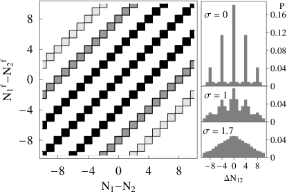
Figure 2: Left panel: Distribution of the final difference $N_{1}^{f}-N_{2}^{f}$ as a function of the initial number difference $N_{1}-N_{2}$ (the darkest area of this contour plot corresponds to the highest probability) for $N_{1}\approx N_{2}\approx 10^{3}$. Right panel: Probability distribution $P$ of $\Delta N_{12}$ (final-state number difference centered at the initial state number difference), assuming Poissonian distributions of the initial atom numbers around mean values $\bar{N}_{1}=1000$ and $\bar{N_{2}}=1000$. The plots are labeled by the total r.m.s. error $\sigma$ of the number measurement. For both panels the number of outcoupled atoms $\nu=26$ and $\langle\cos\phi\rangle=0$.

In Fig. 1(b) we present our QMC simulation of the outcoupling of $\nu$ atoms to the level 0, starting from the state (4) and detecting them one by one. The output of the numerical simulations was twofold: Firstly, we obtained the set of time intervals $\tau_{i}$, $i=1,\,2,\,\dots,\,\nu$, between consecutive detection events. Secondly, we monitored the state of the remaining atoms after each outcoupling event. The average time interval $\bar{\tau}$ was found to be in very good agreement with its estimation $[2WN(1+\langle\cos\phi\rangle)]^{-1}$, where $\langle\cos\phi\rangle$ is the mean value of the $\cos\hat{\phi}$ operator in the state emerging after the outcoupling of the last atom in the measured sequence and $W=V^{2}/\gamma$. The statistical distribution of sequences of $\tau_{i}$ in each QMC run was found to be very close to Poissonian, with the probability density $\bar{\tau}^{-1}\exp(-\tau/\bar{\tau})$. This implies that the first few measurements of $\tau$ determine quite well the value of $\langle\cos\phi\rangle$ and, hence, the subsequent evolution of the system [see inset to Fig. 1(b)].

To prove the MQS nature of the final state, one has to observe the interference structure in the distribution of the final atom-number difference, the variable conjugate to $\phi$. To this end, we plot in Fig. 2 the probability distribution $P(\Delta N^{f})$ of atom number difference in the final state $\Delta N^{f}=N_{1}^{f}-N_{2}^{f}$, as a function of the initial number difference $\Delta N=N_{1}-N_{2}$. The peaks in the distribution of $\Delta N^{f}$ are separated by four atom counts, thus indicating interference effects in the MQS state. The position of these interference peaks depends on the initial number difference, as shown in Fig. 2 (left panel).

If we start with a mixed initial state, characterized by independent Poissonian fluctuations of $N_{1}$, $N_{2}$ around their mean values $\bar{N}_{1}$, $\bar{N}_{2}$, then the interference patterns can be recognized by looking at the quantity $\Delta N_{12}=N_{1}^{f}-N_{2}^{f}-(N_{1}-N_{2})$, the final atom-number difference centered at the initial number difference. This interference structure still persists for a measurement error of 1 atom in determining $\Delta N_{12}$, $\sigma(\Delta N_{12})=1.0$, but disappears for $\sigma(\Delta N_{12})=1.7$.

Such a high sensitivity of the MQS state detection to the accuracy of counting the atoms seems to be a common feature of measurement-based MQS phase-state creation methods (cf. Ref.NB ). Non-demolition measurements of atom-number differences in high-$Q$ cavities QND or quantum culling techniques cull may help satisfy this stringent requirement.

There are different possibilities to realize the $\Lambda$-scheme excitation. Preferably, the level 0 is to be excited via coupling to the ground-state sublevels by laser-induced single-photon transitions. In this case, to avoid complications resulting from co-operative, bosonic-enhanced relaxation jcr , we assume that $N_{1}+N_{2}\ll(k_{L}R)^{2}$, where $k_{L}$ is the laser radiation wavenumber and $R$ is the BEC size. The BEC should be collisionally thin, i.e., the number of collisions per atom moving with the momentum $\sim\hbar k_{L}$ imparted by a scattered photon should be negligible.

Our method can be efficiently implemented with ⁸⁷Rb condensates. The triplet and singlet $s$-wave scattering lengths are very close to each other for this isotope, and therefore inter- and intracomponent scattering length difference for ⁸⁷Rb is of about 1 % Rba . This provides several advantages. Firstly, quantum diffusion of $\phi$ due to slight difference in the mean-field interaction energies for the different states will destroy the intercomponent phase coherence on a very long time scale $\sim 1$ s, if we assume the following parameters: total number of atoms is about 2000, the BEC size $R\approx 10~{}\mu$m. Secondly, the inelastic losses in ⁸⁷Rb are suppressed due to the closeness of the triplet and singlet scattering lengths Rba and can be totally neglected for the given BEC parameters on time scales up to 0.1 s. Additionally, in such a small BEC, bosonic enhancement jcr does not significantly affect the relaxation of the optically excited state, and the probability of a collision for an atom that acquires recoil velocity after scattering a photon is of the order of 0.01. Hence, a few dozens of atoms can be outcoupled without destroying the remaining BEC by collisions.

The collisions with thermal atoms and scattering of resonance stray photons dnm destroy the macroscopic coherence. In general, the rate for the MQS destruction is $(N_{1}+N_{2})$ faster than the rate of excitation of an individual atom from the condensate (we assume that every such scattering is energetic enough to change the translational state of atomic motion). Since the lifetimes of a BEC of the order of several tens of seconds are experimentally feasible, an MQS can persist in a system with $N_{1}\approx N_{2}\sim 10^{3}$ for tens of milliseconds, which is long enough to perform the necessary optical manipulation and detection steps whose duration lies in the sub-millisecond range.

To conclude, we have proposed a novel method for creating macroscopic superposition states in two-component BECs by measuring the cosine of the intercomponent phase. Either “snapshot” detection of the number of outcoupled atoms or their continuous observation have been shown to yield the desired result (Fig. 1). This method allows for fluctuations of the atom-number difference in the initial state, if the error in atom counting by a detector is maintained at the level of $\pm 1$ atom (Fig. 2). Each measurement of $\cos\phi$ yields a MQS, provided that the measured $\phi$ is not too close to 0 or $\pm\pi$. In particular, for the parameters of Fig. 2 (right panel), the peaks in two-peaked phase distribution appear to be well-resolved if $|\langle\cos\phi\rangle|<0.3$. This distinguishes our method from the method of optical MQS generation recently developed ourj for homodyne measurements of quantum field quadratures that are suitable for photons, but not for atoms. A major advantage of our method compared to methods based on nonlinear interactions in the system itself dnm ; mpr ; zl ; zurek is that it allows one to create MQS rapidly enough, regardless of the nonlinearity smallness, well before the interaction with the environment brings about the collapse of the macroscopic superposition.

This work is supported by the German-Israeli Foundation, the EC (MIDAS STREP) and INTAS (project 06–1000013–9427). I.E.M. acknowledges the Lise Meitner Fellowship by the FWF.

References

- (1) Schrödinger E., Naturwiss. 23 (1935) 807; ibid., 823; ibid., 844.
- (2) Bollinger J.J., Itano W.M., Wineland D.J., and Heinzen D.J., Phys. Rev. A 54 (1996) R4649.
- (3) Liebfried D. et al., Nature 438 (2005) 639.
- (4) Brune M. et al., Phys. Rev. Lett. 77 (1996) 4887.
- (5) Monroe C., Meekhof D.M., King B.E., and Wineland D.J., Science 272 (1996) 1131.
- (6) Friedman J.R., Sarachik M.P., Tejada J., and Ziolo R., Phys. Rev. Lett. 76 (1996) 3830.
- (7) Rouse R., Han S., and Lukens J.E., Phys. Rev. Lett. 75 (1995) 1614; Nakamura Y., Pashkin Y.A., and Tsai J.S., Nature 398 (1999) 786; Friedman J.R. et al., Nature 406 (2000) 43.
- (8) Yurke B. and Stoler D., Phys. Rev. Lett. 57 (1986) 13.
- (9) Albiez M. et al., Phys. Rev. Lett. 95, (2005) 010402; Gati R. and Oberthaler M.K., J. Phys. B 40 (2007) R61.
- (10) Huang Y.P. and Moore M.G., Phys. Rev. A 73 (2006) 023606.
- (11) Mahmud K.W., Perry H., and Reinhardt W.P., J. Phys. B 36 (2003) L265.
- (12) Micheli A., Jaksch D., Cirac J.I., and Zoller P., Phys. Rev. A 67 (2003) 013607.
- (13) Dalvit D.A.R., Dziarmaga J., and Zurek W.H., Phys. Rev. A 62 (2000) 013607.
- (14) Massar S. and Polzik E.S., Phys. Rev. Lett. 91 (2003) 060401.
- (15) E. Arimondo, in Progress in Optics, ed. E. Wolf, vol. 35, Elsevier, Amsterdam (1995), p. 257.
- (16) Smerzi A., Fantoni S., Giovanazzi S., and Shenoy S.R., Phys. Rev. Lett. 79 (1997) 4950.
- (17) Castin Y. and Dalibard J., Phys. Rev. A 55 (1997) 4330.
- (18) Ruostekoski J., Collett M.J., Graham R., and Walls D.F., Phys. Rev. A 57 (1998) 511.
- (19) Dunningham J.A., Burnett K., Roth R., and Phillips W.D., New J. Phys., 8 (2006) 182.
- (20) Pegg D.T. and Barnett S.M., Europhys. Lett. 6 (1988) 483; Luis A. and Sánchez-Soto L.L., Phys. Rev. A 48 (1993) 4702.
- (21) Morigi G., Zambon B., Leinfellner N. and Arimondo E., Phys. Rev. A 53 (1996) 2616.
- (22) Javanainen J. and Yoo S.M., Phys. Rev. Lett. 76 (1996) 161.
- (23) If one tunes a high- cavity resonance inbetween the two hyperfine ground states, then one can directly measure the atom-number difference between the two states in the strong coupling regime of cavity-trapped atoms, see: F. Brennecke et al., Nature 450 (2007) 268; Colombe Y. et al., Nature 450 (2007) 272.
- (24) Dudarev A.M., Raizen M.G., and Qian Niu, Phys. Rev. Lett. 98 (2007) 063001.
- (25) Javanainen J., Phys. Rev. Lett. 72 (1994) 2375.
- (26) Burke J.P., Jr., Bohn J.L., Esry B.D., and Greene C.H., Phys. Rev. Lett. 80 (1998) 2097.
- (27) Ourjoumtsev A., Jeong H., Tualle-Brouri R. and Grangier P., Nature 448 (2007) 784.