External Momentum, Volume Effects, and the Nucleon Magnetic Moment

Abstract

We analyze the determination of volume effects for correlation functions that depend on an external momentum. As a specific example, we consider finite volume nucleon current correlators, and focus on the nucleon magnetic moment. Because the multipole decomposition relies on $SO(3)$ rotational invariance, the structure of such finite volume corrections is unrelated to infinite volume multipole form factors. One can deduce volume corrections to the magnetic moment only when a zero-mode photon coupling vanishes, as occurs at next-to-leading order in heavy baryon chiral perturbation theory. To deduce such finite volume corrections, however, one must assume continuous momentum transfer. In practice, volume corrections with momentum transfer dependence are required to address the extraction of the magnetic moment, or other observables that arise in momentum dependent correlation functions. Additionally we shed some light on a puzzle concerning differences in lattice form factor data at equal values of momentum transfer squared.

I Introduction

QCD in the non-perturbative regime has proven notoriously difficult to understand quantitatively. This non-Abelian gauge theory of gluons coupled to quarks is simple enough to write down, and even becomes perturbative at high energies. At low energies, however, the theory is strongly coupled which results in the confinement of quarks and gluons into hadrons. Accounting for the measured properties of hadrons is a challenge; making reliable predictions is even more difficult. After more than a quarter century of dedicated work, lattice gauge theory has made considerable progress in addressing strong interaction physics. As a first principles numerical technique, lattice gauge theory can be used to determine low-energy hadronic properties rigorously from QCD. For a comprehensive overview of lattice methods, see DeGrand and DeTar (2006)

Despite considerable success, lattice QCD calculations still suffer from a number of systematic errors. Due to computational restrictions, simulations cannot be carried out at the physical pion mass. Instead heavier pions must be used. Additionally current lattice volumes are not significantly larger than the typical hadronic length scale, which for most observables is set by the pion Compton wavelength. To eliminate such systematic errors, it is desirable to have an independent tool that predicts the pion mass, and lattice volume dependence of observables. Fortunately, effective field theory techniques exist suited for this purpose. Chiral perturbation theory, for example, provides a model independent and systematic tool to address the pion mass and lattice volume dependence of many low-energy hadronic properties. Pioneering work on the volume dependence of the chiral condensate and pion observables appeared a while ago in series of papers Gasser and Leutwyler (1987a, b); Leutwyler (1987); Gasser and Leutwyler (1988). Additionally finite volume amplitudes have been analyzed in order to study unstable particles and multiparticle physics Luscher (1991b, a); Lellouch and Luscher (2001). A variety of observables have since been treated in finite volume. Recent work has included treating heavy mesons and baryons Ali Khan et al. (2004); Arndt and Lin (2004); Beane (2004); Beane and Savage (2004); Bernard et al. (2007), extending the validity of finite volume corrections for meson masses and decay constants Colangelo and Haefeli (2004); Colangelo et al. (2005); Colangelo and Haefeli (2006), exploring different regimes in finite volume theories Detmold and Savage (2004); Bedaque et al. (2005); Smigielski and Wasem (2007), and investigating multiparticle systems in finite volume Beane et al. (2004); Bedaque et al. (2006); Sato and Bedaque (2007); Beane et al. (2007).

Further work at finite volume has included processes depending on an external momentum Detmold and Lin (2005); Bunton et al. (2006); Chen et al. (2007); Detmold et al. (2006). Deducing volume corrections to electromagnetic observables, for example, can be a subtle task Hu et al. (2007a, b). A point that was specifically addressed in these latter works was the lacking connection of finite volume amplitudes to low-energy multipole expansions. Multipole expansions are inherent in the description of $SO(3)$ invariant physics. At finite volume such a description of low-energy matrix elements ceases to be valid. Utilizing effective field theory, finite volume corrections to amplitudes can be computed, but not corrections to multipole moments and other observables, such as multipole polarizabilities. Said another way, an effective field theory only allows one to match the calculation of correlation functions. Thus chiral perturbation theory allows one to calculate the model-independent, long-distance behavior of finite volume correlation functions. Connection to infinite volume observables, which might be accessible through various different correlation functions, is not mandated.

In this work, we consider finite volume correlation functions depending on an external momentum. Specifically, we detail the finite volume modifications to nucleon current matrix elements, and analyze whether it is possible to deduce volume corrections to the nucleon magnetic moment. Based on symmetry considerations, we show that such a connection to infinite volume physics is not generally possible; but, within the framework of heavy baryon chiral perturbation theory, the vanishing of a new finite volume coefficient at next-to-leading order allows for the connection to be made. We are careful to expose, however, that this analysis relies on the assumption of continuous momentum transfer. On the lattice, the available momentum modes are quantized, but there is a regime in which the assumption of continuous momentum is approximately valid. This regime, however, is beyond the reach of current computing resources. Thus in practice, the volume effect must be determined from the momentum transfer dependent nucleon current matrix element. Although we have specialized to current matrix elements, our analysis generalizes to any momentum-dependent correlation function at finite volume. Finally using our expressions for current matrix elements, we show that form factors calculated at equal values of momentum transfer squared (but at differing momentum transfer) can differ due to volume effects. This potentially resolves a puzzle seen in lattice form factor data.

Our presentation has the following organization. In Sect. II, we write down the single particle effective action for the nucleon coupled to an electromagnetic field. This is done for a spatial torus. Here we show based on symmetry arguments that the electromagnetic current is additively renormalized, and that there is an additional magnetic-like zero-mode interaction. Next in Sect. III, we calculate polarized nucleon electromagnetic current matrix elements in finite volume. Heavy baryon chiral perturbation theory is utilized, and the relevant finite volume functions appearing in the calculation are listed in Appendix A. The results of this calculation can be used to determine the volume-dependent coupling constants in the single nucleon effective action. In Sect. IV, we investigate the conditions necessary for the matching to be performed, and find they require lattice sizes larger than currently available. In Appendix B, we carry out the momentum expansion one non-trivial order further to discuss the magnetic radius at finite volume. The form factor difference puzzle is taken up in Sect. IV.3. Generic features of our findings are summarized in Sect. V.

II Single Particle Effective Action

We begin by considering the low-energy dynamics of a nucleon in an external electromagnetic field. We use a two component isospinor $N$ for the nucleon. In infinite volume the nucleon can be described by the Lagrangian

$${\mathcal{L}}={\overline{N}}\left(iv\cdot D-\frac{D_{\perp}^{2}}{2M_{N}}-\frac{i\mu_{N}}{2M_{N}}\left[S_{\mu},S_{\nu}\right]F^{\mu\nu}\right)N,$$ (1)

where $v^{\mu}$ is the heavy nucleon four-velocity, $S^{\mu}$ is the covariant spin operator, and $D_{\perp}^{\mu}=D^{\mu}-v^{\mu}(v\cdot D)$, see Jenkins and Manohar (1991). The coefficient of the kinetic term is exactly fixed by reparametrization invariance Luke and Manohar (1992), but the form of the operator is unique only up to field redefinitions. The gauge covariant derivative appearing above is $D_{\mu}=\partial_{\mu}+ieQ_{N}A_{\mu}$, where $Q_{N}$ is the nucleon charge matrix. The coupling constant $\mu_{N}$ is a diagonal matrix containing the proton and neutron magnetic moments. In writing the above Lagrangian, we have included all zeroth and first order terms in an expansion in photon frequency. At higher order in the frequency expansion, there are terms with more powers of the field strength tensor, $F^{\mu\nu}$, and derivatives thereof. Because we work well below the pion production threshold, we have integrated out pion-nucleon interactions to arrive at Eq. (1). The low-energy constants in the matrix $\mu_{N}$ depend on the pion mass and other couplings of the nucleon theory with pion interactions. That theory is chiral perturbation theory, and we treat such dependence as implicit.

In finite volume, we can write down a theory analogous to Eq. (1). To be concrete, we assume that this theory is defined on a torus of length $L$ in each of the three spatial directions. This reflects the underlying lattice QCD action with quarks subject to periodic boundary conditions, but ignoring any possible effect from the finite time direction. The general form of the single nucleon effective action can be constructed by writing down all possible operators consistent with the symmetries of electromagnetism on a torus. The discrete symmetries $C$, $P$, and $T$ remain. Boost invariance and $SO(3)$ rotational invariance possessed by the Lagrangian in Eq. (1), however, are reduced to the cubic symmetry group, which is isomorphic to $S_{4}$. On compactified spaces, gauge transformations are more constrained for the gauge field zero mode. A well known example of this occurs in finite temperature gauge theory, see, e.g. Zinn-Justin (1996). On the spatial torus we consider, the zero modes of the three-vector potential have periodicity constraints under gauge transformations. This restriction on gauge transformations leads to the ability to construct more gauge invariant operators than in infinite volume.

In Hu et al. (2007a), the spatial analog of the Polyakov line was used to write down gauge invariant operators involving the gauge field zero modes. Specifically employed was the Wilson line ${\mathcal{W}}_{i}$ defined by

$${\mathcal{W}}_{i}=\exp\left(\frac{ie}{3}\oint dx_{i}\,A_{i}\right),$$ (2)

where the line integral starts at some point $x_{\mu}$ and runs to $x_{\mu}+L\hat{x}_{i}$. There is no implied sum over $i$ on the right-hand side of Eq. (2). Because the gauge potential is periodic, cycling the compact dimension must produce a gauge invariant object. The factor of $e/3$ reflects that the quark charges are quantized in such units. Under a gauge transformation, we have $A^{\mu}\to A^{\mu}+\partial^{\mu}\alpha$. In order for the Wilson line in Eq. (2) to be gauge invariant, we must have

$$\alpha(x_{i}=L)=\alpha(x_{i}=0)+\frac{6\pi}{e}n_{i},$$ (3)

where $n_{i}$ is an integer. As this condition must hold in each spatial direction, we find

$$\alpha(x)=\frac{6\pi}{eL}\bm{n}\cdot\bm{x}+{\overline{\alpha}}(x),$$ (4)

where ${\overline{{\alpha}}}(x)$ is a periodic function of the $x_{i}$. The linear term in the gauge function ${\alpha}(x)$ gives rise to a quantized shift of the gauge field zero mode.

To write an effective theory of the nucleon and photons in finite volume, it is easiest to use linear combinations of Wilson lines that are Hermitian and have definite $C$, $P$, and $T$ transformations. These are the operators ${\mathcal{W}}_{i}^{(+)}$, and ${\mathcal{W}}_{i}^{(-)}$ given by

$${\mathcal{W}}_{i}^{(+)} = \frac{1}{2}\left({\mathcal{W}}_{i}+{\mathcal{W}}_{i}^{\dagger}\right),$$ (5)

$${\mathcal{W}}_{i}^{(-)} = \frac{1}{2i}\left({\mathcal{W}}_{i}-{\mathcal{W}}_{i}^{\dagger}\right).$$ (6)

It is easy to show that these two operators are not independent, and we choose to work with the ${\mathcal{W}}_{i}^{(-)}$ because they have the same $C$, $P$, and $T$ symmetry transformations as the $A_{i}$. Constructing the most general gauge invariant Lagrangian on a torus is arbitrarily complicated. As our interest is with the nucleon magnetic moment, we restrict our attention to operators having only one insertion of ${\mathcal{W}}_{i}^{(-)}$. Multiple insertions of ${\mathcal{W}}_{i}^{(-)}$ lead to photon-nucleon couplings with more than one photon. Furthermore we restrict our attention to operators with at most one derivative. We will investigate the conditions that justify such a photon frequency expansion in Sect. IV.

We now build the single particle effective action for nucleons and photons on a torus. To write this theory, we abandon the covariant notation employed in Eq. (1) above, because the torus has only $S_{4}$ invariance. Including all single ${\mathcal{W}}^{(-)}_{i}$ operators with at most one derivative, we have the Lagrangian

$${\mathcal{L}}={\overline{N}}\left[iD_{0}+\frac{\bm{D}^{2}}{2M_{N}}-\frac{C_{1}(L)}{2M_{N}}i\overset{\leftrightarrow}{\bm{D}}\cdot\bm{{\mathcal{W}}}^{(-)}+\frac{\mu_{N}(L)}{2M_{N}}\,\bm{\sigma}\cdot\bm{B}+\frac{C_{2}(L)}{2M_{N}}\,\bm{\sigma}\cdot\left(\bm{\nabla}\times\bm{{\mathcal{W}}}^{(-)}\right)\right]N,$$ (7)

where $i\overset{\leftrightarrow}{\bm{D}}=i\left(\overset{\leftarrow}{\bm{D}}-\overset{\rightarrow}{\bm{D}}\right)$ defines an Hermitian operator. Notice that $\nabla_{i}{\mathcal{W}}^{(-)}_{i}=0$. In writing Eq. (7), we have explicitly indicated the dependence on the spatial length $L$. The coupling constants above run with the infrared cutoff, $1/L$, and must be determined by matching calculations in the microscopic theory. For example, the magnetic moment operator is accompanied by the finite volume coefficient $\mu_{N}(L)$ which is given by

$$\mu_{N}(L)=\mu_{N}+\delta\mu_{N}(L),$$ (8)

where the term $\delta\mu_{N}(L)$ is the finite volume effect that can be determined using chiral perturbation theory. Running the infrared cutoff to zero produces the infinite volume magnetic moment, $\underset{L\to\infty}{\lim}\mu_{N}(L)=\mu_{N}$. Compared to Eq. (1), there are two new operators allowed by symmetry. These operators contain single photon couplings as well as a tower of cubic invariant multi-photon couplings. There are, however, further multi-photon operators that we have not written in Eq. (7). Such operators involve multiple insertions of ${\mathcal{W}}^{(-)}_{i}$. The new coupling constants $C_{1}(L)$ and $C_{2}(L)$ appearing in Eq. (7) both must run to zero when the infinite volume limit is taken. As we work below any multi-particle thresholds, these $L$-dependent couplings run to zero exponentially fast in asymptotically large volumes Luscher (1991a). Notice that expanding the Lagrangian in Eq. (7) to linear order in the gauge field, we have an accidental $SO(3)$ invariance.

The effective theory in Eq. (7) can be used to calculate single photon-nucleon processes. For example, for an unpolarized nucleon at rest, we have the current matrix element

$$\langle N(\bm{0})|J^{\mu}|N(\bm{0})\rangle=Q_{N}\,e\,g^{\mu 0},$$ (9)

which produces the total charge. In infinite volume, we can boost this result to an inertial frame where the nucleon moves with momentum $\bm{p}=M_{N}\,\bm{v}$. By Galilean invariance, we expect the current to be $\bm{j}=Q_{N}e\bm{v}$. Using Eq. (7) to calculate the current in this frame, however, yields

$$\langle N(\bm{p})|\bm{J}|N(\bm{p})\rangle=[Q_{N}-{\mathcal{Q}}_{N}(L)]e\bm{v},$$ (10)

where ${\mathcal{Q}}_{N}(L)=L\,C_{1}(L)/3$. The electromagnetic current has been additively renormalized by the operator with coefficient $C_{1}(L)$. The theory described by Eq. (7) is not Galilean invariant. This is the non-relativistic analog of Lorentz symmetry violation on a torus that allows current renormalization described in Hu et al. (2007a). The sign in Eq. (7) [and consequently that in Eq. (10)] anticipates that the infinite volume current is screened in finite volume.

We can further apply the effective Lagrangian in Eq. (7) to polarized matrix elements. For a momentum transfer of $\bm{q}=\frac{2\pi}{L}\bm{n}$, we find

$$\langle N(\bm{q})\downarrow|J_{k}|N(\bm{0})\downarrow\rangle-\langle N(\bm{q})\uparrow|J_{k}|N(\bm{0})\uparrow\rangle=\frac{i\varepsilon_{3jk}q_{j}}{M_{N}}\left[\mu_{N}(L)+\delta_{n_{k},0}\,{\overline{\mu}}_{N}(L)\right],$$ (11)

which is sensitive to the finite volume magnetic moment and the additional zero-mode coupling ${\overline{\mu}}_{N}(L)$, which is given by ${\overline{\mu}}_{N}(L)=eL\,C_{2}(L)/3$. To determine the volume dependent couplings, we must match finite volume chiral perturbation theory calculations onto the single nucleon effective action in Eq. (7). We now turn to these calculations.

III Heavy Baryon Calculation

III.1 Chiral Perturbation Theory

To determine volume corrections to photon-nucleon couplings, we utilize heavy baryon chiral perturbation theory. The virtual pion cloud of the nucleon deforms in finite volume because pions are the lightest hadrons, and easily propagate to the boundary. Their small masses arise because pions are the pseudo-Goldstone bosons arising from spontaneous chiral symmetry breaking. For the case of two flavors, the symmetry breaking pattern is from $SU(2)_{L}\otimes SU(2)_{R}\to SU(2)_{V}$, and the Goldstone manifold is parametrized by the coset field ${\Sigma}\equiv\xi^{2}=\exp(2i\phi/f)$, where the $SU(2)$ matrix $\phi$ contains the pions

$$\phi=\begin{pmatrix}\frac{1}{\sqrt{2}}\pi^{0}&&\pi^{+}\\ \pi^{-}&&-\frac{1}{\sqrt{2}}\pi^{0}\end{pmatrix}.$$ (12)

At leading order, ${\mathcal{O}}(\varepsilon^{2})$, in a small momentum, $p$, and pion mass, $m_{\pi}$ expansion, where $\varepsilon\sim p\sim m_{\pi}$, the theory of pions is described by the Lagrangian

$${\mathcal{L}}=\frac{f^{2}}{8}\left[\text{tr}(D_{\mu}{\Sigma}D^{\mu})+m_{\pi}^{2}\,\text{tr}({\Sigma}+{\Sigma}^{\dagger})\right].$$ (13)

Here we work in the isospin limit, and at tree level $m_{\pi}$ is the physical pion mass. The dimensionful parameter $f$ is the pion decay constant, $f=132\,\texttt{MeV}$. Electromagnetism has been gauged into Eq. (13) via the covariant derivative $D^{\mu}=\partial^{\mu}+ieA_{\mu}[Q,\,\,\,]$, where $Q$ is the quark electric charge matrix

$$Q=\text{diag}\left(\frac{2}{3},-\frac{1}{3}\right).$$ (14)

To include baryons we use the isospinor $N$ from above,

$$N=\begin{pmatrix}p\\ n\end{pmatrix},$$ (15)

as well as the heavy baryon formulation which allows us a consistent expansion in powers of residual momentum, $k_{\mu}\sim\varepsilon$, where we decompose an arbitrary nucleon momentum $P$ into $P_{\mu}=M_{N}\,v_{\mu}+k_{\mu}$. To leading order, ${\mathcal{O}}(\varepsilon)$, the heavy baryon chiral Lagrangian is

$${\mathcal{L}}={\overline{N}}\left(iv\cdot D+2g_{A}S\cdot{\mathcal{A}}\right)N,$$ (16)

where ${\mathcal{A}}_{\mu}$ and ${\mathcal{V}}_{\mu}$ are axial-vector and vector pion fields defined by

$${\mathcal{A}}_{\mu} = \frac{i}{2}\left(\xi\partial_{\mu}\xi^{\dagger}-\xi^{\dagger}\partial_{\mu}\xi\right),$$ (17)

$${\mathcal{V}}_{\mu} = \frac{1}{2}\left(\xi\partial_{\mu}\xi^{\dagger}+\xi^{\dagger}\partial_{\mu}\xi\right),$$ (18)

the latter appears in the chirally and electromagnetically gauge covariant derivative $D_{\mu}$, which acts on the nucleon isospinor as

$$D_{\mu}N=\left(\partial_{\mu}+{\mathcal{V}}_{\mu}+ieQ_{N}A_{\mu}\right)N.$$ (19)

The nucleon charge matrix $Q_{N}$ is given by $Q_{N}=Q+\text{tr}\,Q$.

The nearest baryon resonances in the spectrum of QCD are the deltas. Phenomenologically we know the nucleon-delta axial couplings are not small. Furthermore the nucleon-delta mass splitting $\Delta\sim 300\,\texttt{MeV}$ is not much greater than the pion mass. In fact on current lattices, the lightest lattice pion masses are the same size as $\Delta$. Hence for a consistent power counting, we must treat $\Delta\sim\varepsilon$, and retain deltas in the theory as explicit degrees of freedom. The deltas are described by the flavor tensor field $T_{\mu}$, which is heavy baryon Rarita-Schwinger spinor. The leading order, ${\mathcal{O}}({\varepsilon})$, Lagrangian for the deltas and their interactions with nucleons is given by

$${\mathcal{L}}=-{\overline{T}}{}^{\mu}\left(iv\cdot D-\Delta\right)T_{\mu}+g_{\Delta N}\left({\overline{T}}{}^{\mu}{\mathcal{A}}_{\mu}N+{\overline{N}}{\mathcal{A}}^{\mu}T_{\mu}\right)+2g_{\Delta\Delta}{\overline{T}}{}^{\mu}S\cdot{\mathcal{A}}T_{\mu}.$$ (20)

III.2 Magnetic Form Factor

Having spelled out the interactions of nucleons with pions and deltas, we detail the calculation of the magnetic form factor in infinite volume. Consider the polarized nucleon matrix elements that define the Pauli form factor

$$\langle N(\bm{q})\downarrow|J_{k}|N(\bm{0})\downarrow\rangle-\langle N(\bm{q})\uparrow|J_{k}|N(\bm{0})\uparrow\rangle=\frac{iq_{j}\varepsilon_{3jk}}{M_{N}}F_{2}(q^{2}).$$ (21)

The magnetic moment is given by the form factor at zero momentum transfer

$$\mu_{N}=F_{2}(0).$$ (22)

In the heavy baryon theory, contributions to $F_{2}(q^{2})$ arise from local photon-nucleon interactions, as well as from virtual pion loop contributions generated by leading-order Lagrangian. The leading contribution to magnetic moments come from the local interactions at ${\mathcal{O}}({\varepsilon}^{0})$. These are contained in the current operator

$$J^{\mu}=-\frac{i\partial_{\nu}}{M_{N}}\left(\mu_{0}{\overline{N}}[S^{\mu},S^{\nu}]N+\mu_{I}{\overline{N}}[S^{\mu},S^{\nu}]\tau^{3}N\right),$$ (23)

where $\tau^{3}$ is an isospin matrix. The two terms above contribute to the isoscalar and isovector moments, respectively. For simplicity we shall address the isovector magnetic moment and isovector Pauli form factor. These are defined simply as proton minus neutron differences in these respective quantities.

Higher order corrections to the Pauli form factor come from loop diagrams generated from the leading order Lagrangian in Eqs. (16), and (20). Specifically the one loop graphs for the Pauli form factor are depicted in Figure 1. These graphs make ${\mathcal{O}}({\varepsilon})$ contributions to magnetic moments.

Figure 1: Loop diagrams contributing to the nucleon magnetic moments at ${\mathcal{O}}({\varepsilon})$. The photon is depicted as a wiggly line, mesons are denoted by a dashed line, and a thin solid line denotes a nucleon, while the double line denotes a delta.

Evaluation of these diagrams, combined with the tree-level result yields the isovector Pauli form factor $F_{2}^{(I)}(q^{2})$ Jenkins et al. (1993); Bernard et al. (1992, 1998),

$$F_{2}^{(I)}(q^{2})=2\mu_{I}-\frac{g_{A}^{2}M_{N}}{2\pi f^{2}}\int_{0}^{1}dx\,m_{\pi}P_{\pi}(x,q^{2})-\frac{g_{\Delta N}^{2}M_{N}}{9\pi^{2}f^{2}}\int_{0}^{1}dx\,F[m_{\pi}P_{\pi}(x,q^{2}),\Delta],$$ (24)

where

$$P_{\pi}(x,q^{2})=\sqrt{1-x(1-x)\frac{q^{2}}{m_{\pi}^{2}}},$$ (25)

encodes the momentum transfer dependence, and the non-analytic function $F(m,\delta)$ is given by

$$F(m,\delta)=-\delta\log\left(\frac{m^{2}}{4\delta^{2}}\right)+\sqrt{\delta^{2}-m^{2}}\log\left(\frac{\delta-\sqrt{\delta^{2}-m^{2}}+i\epsilon}{\delta+\sqrt{\delta^{2}-m^{2}}+i\epsilon}\right).$$ (26)

In order to arrive at this answer we have renormalized the tree-level coupling $\mu_{I}$, so that at one-loop order the $\mu_{I}$ in Eq. (24) is the chiral limit value.

III.3 Finite Volume Form Factor

We now consider the finite volume modifications to the isovector Pauli form factor. We delay the determination of volume corrections to the magnetic moment until Sect. IV. To calculate volume corrections, we use the same setup as described in Sect. II, namely we take a finite space of volume $L^{3}$ with an infinite time extent. The pions, nucleons, and deltas, moreover, have periodic boundary conditions which stem from the periodicity of quarks in the lattice action, and the fact that hadron fields are point-like objects in the effective theory.

To calculate observables in the finite volume theory we use the Lagrangian in Eqs. (13), (16), and (20). The action, however, is given by the volume intergral of the Lagrangian with periodic boundary conditions on all fields enforced. Thus the same Feynman diagrams are generated in the finite volume theory as in infinite volume. The difference is the spatial momentum quantization of internal and external lines. We must further choose $m_{\pi}L\gg 1$ so that the zero mode of the pion field does not become strongly coupled Gasser and Leutwyler (1987a, b). With this assumption on the lattice size $L$, the $\varepsilon$ power counting we have employed in infinite volume carries over to finite volume Gasser and Leutwyler (1988).

The volume correction to the nucleon current matrix element, $\delta\langle N|J^{\mu}|N\rangle_{L}$, can be determined by a trivial matching condition, namely

$$\langle N|J^{\mu}|N\rangle_{L}=\langle N|J^{\mu}|N\rangle_{\infty}+{\delta}\langle N|J^{\mu}|N\rangle_{L},$$ (27)

where $\langle N|J^{\mu}|N\rangle_{L}$ is the finite volume current matrix element, and $\langle N|J^{\mu}|N\rangle_{\infty}$ is the infinite volume result, e.g. the isovector magnetic contribution shown in Eq. (24). We have temporarily suppressed the momentum transfer argument and denote $L$-dependence with subscripts rather than parenthetically. Because the finite and infinite volume theories share exactly the same ultraviolet divergences, the matching condition above ensures that ${\delta}\langle N|J^{\mu}|N\rangle_{L}$ is indeed the infrared effect.

Carrying out the matching in Eq. (27) on the spatial isovector current matrix element, we find

$${\delta}\langle N(\bm{q})|J^{i}_{\text{Iso}}|N(\bm{0})\rangle_{L} = -\frac{3}{f^{2}}\left[g_{A}^{2}f^{ij}(q^{2},\bm{q},0)+\frac{2}{9}g_{{\Delta}N}^{2}f^{ij}(q^{2},\bm{q},{\Delta})\right]\,{\overline{u}}\left[S^{j},\bm{S}\cdot\bm{q}\right]u,$$ (28)

where we have defined the function

$$f^{ij}(q^{2},\bm{q},{\delta})=\int_{0}^{1}dx\left\{2I^{ij}_{5/2}[x\bm{q},m_{\pi}P_{\pi}(x,q^{2}),{\delta}]+q^{i}I^{j}_{5/2}[x\bm{q},m_{\pi}P_{\pi}(x,q^{2}),{\delta}]\right\},$$ (29)

in terms of $I^{i}_{\beta}(\bm{{\theta}},m,{\delta})$, and $I^{ij}_{\beta}(\bm{{\theta}},m,{\delta})$ which are finite difference functions appearing in the Appendix. The $u$, and ${\overline{u}}$ appearing in Eq. (28) are Pauli spinors, and $P_{\pi}(x,q^{2})$ is given in Eq. (25).

From Eq. (28), we cannot identify finite volume corrections to the Pauli form factor. Indeed the form factor decomposition of nucleon current matrix elements is tied to Lorentz and gauge invariance. The former does not hold on a torus, while the latter has a completely different form. The integrand of Eq. (29) is clearly an even function of each component of $\bm{q}$. More generally it is a cubic invariant function of the spatial momentum, and so depends on $\bm{q}^{2}$, as well as $\sum_{i}q_{i}q_{i}q_{i}q_{i}$, and a tower of other cubic invariant combinations. As there is no simple way to denote this, we have chosen simply to write $f^{ij}=f^{ij}(q^{2},\bm{q},{\delta})$. This function should be considered as a finite volume generalization of a form factor.

With Eq. (28), we have determined volume corrections to nucleon current matrix elements. This result can be directly utilized to remove volume dependence from lattice calculations of the nucleon current provided one is in the range of applicability of heavy baryon chiral perturbation theory. The expression can be simplified, moreover, depending on the actual lattice kinematics used in measuring the three-point function on the lattice. For example, to be sensitive to the magnetic coupling in Eq. (11), the momentum transfer $\bm{q}$ must have at least one component transverse to the plane of spin polarization. We shall thus assume that $\bm{q}$ has no component parallel to the spin polarization. Additionally from Eq. (11), we see that the spatial component of the current measured must be transverse to the spin polarization. We can thus take $\bm{q}$ and $\bm{J}$ to be mutually orthogonal in the plane transverse to the polarization. This choice is sensitive to the Pauli form factor and simplifies the volume dependence. Because $\bm{q}$ is orthogonal to $\bm{J}$, the second term in the integrand of $f^{ij}(q^{2},\bm{q},{\delta})$ is zero since $i$ labels the index of the current in Eq. (28).

For the sake of concreteness take $\bm{q}=(q,0,0)$ and consider the $y$-component of the current. Then we have the volume effect that we loosely denote by ${\delta}F_{2}^{(I)}(q,L)$ for lack of a better symbol,

$${\delta}F_{2}^{(I)}(q,L) \equiv \frac{M_{N}}{iq}\Big{[}{\delta}\langle N(\bm{q})\downarrow|\hat{\bm{y}}\cdot\bm{J}_{\text{Iso}}|N(\bm{0})\downarrow\rangle_{L}-{\delta}\langle N(\bm{q})\uparrow|\hat{\bm{y}}\cdot\bm{J}_{\text{Iso}}|N(\bm{0})\uparrow\rangle_{L}\Big{]}$$

$$= -\frac{6M_{N}}{f^{2}}\int_{0}^{1}dx\left\{g_{A}^{2}I^{22}_{5/2}[xq\hat{\bm{x}},m_{\pi}P_{\pi}(x,q^{2}),0]+\frac{2}{9}g_{{\Delta}N}^{2}I^{22}_{5/2}[xq\hat{\bm{x}},m_{\pi}P_{\pi}(x,q^{2}),{\Delta}]\right\}.$$

If other kinematics are chosen, one must return to Eq. (28) and evaluate accordingly.

IV Matching and Discussion of Results

Having deduced the finite volume modification to nucleon current matrix element, we can now analyze the volume dependence and make contact with the single particle action in Eq. (7). Connection to the single particle action with spin-dependent higher derivative terms is carried out in Appendix B.

IV.1 Matching

To perform the matching, we return to the volume corrections under the general kinematics, Eq. (28), and series expand in the momentum transfer. To find the leading term, we need to evaluate the finite volume form factor $f^{ij}(q^{2},\bm{q},{\delta})$ at zero momentum,

$$f^{ij}(0,\bm{0},{\delta})=\frac{2}{3}\delta^{ij}J_{5/2}(m_{\pi},{\delta}),$$ (31)

where $J_{\beta}(m,{\delta})$ is given in Appendix A. After some algebra, the leading term in the series expansion of the matrix element can be written as

$${\delta}\langle N(\bm{q})|J^{i}_{\text{Iso}}|N(\bm{0})\rangle_{L} = \frac{1}{M_{N}}{\overline{u}}\left[S^{i},\bm{S}\cdot\bm{q}\right]u\,\,{\delta}F^{(I)}_{2}(0,L)+{\mathcal{O}}(q^{3}),$$ (32)

where $F_{2}^{(I)}(0,L)$ is identical to the function in Eq. (LABEL:eq:start) evaluated at $q=0$. Comparing with Eq. (7), we thus find

$$\mu_{N}^{(I)}(L) = F_{2}^{(I)}(0)+{\delta}F_{2}^{(I)}(0,L)$$ (33)

$$C_{2}(L) = 0.$$ (34)

The term ${\delta}F_{2}^{(I)}(0,L)$ is identified as the finite volume correction to the isovector magnetic moment, ${\delta}\mu_{N}^{(I)}(L)$, and (after algebra) is identical to that determined in Beane (2004). Furthermore the additional magnetic-like zero mode interaction in Eq. (7) vanishes to this order. This is true of both the isovector and isoscalar combinations. The remaining coefficient in Eq. (7), $C_{1}(L)$, must be determined by computing the charge form factor in finite volume. The first non-vanishing contributions are from recoil order ($\sim 1/M_{N}$) terms in they heavy baryon theory.

The finite volume correction to the current matrix element in Eq. (28) is determined at some general value $\bm{q}=2\pi\bm{n}/L$. We must investigate the conditions under which the series expansion in quantized $\bm{q}$ leading to Eq. (32) is justified. For simplicity of notation, consider the momentum to lie entirely in one direction. A derivative expansion of the matrix element is justified as follows. For the $n$-th mode, $q_{n}=2\pi n/L$, and for large enough $n$, the relative difference ${\delta}q$,

$${\delta}q=\frac{q_{n+1}-q_{n}}{q_{n}}=\frac{1}{n},$$ (35)

approaches zero. To rigorously series expand, we must take differences of the nucleon current matrix element between adjacent modes for large mode number. This is the procedure implicitly needed to arrive at Eq. (32). Such a procedure is lacking when one is restricted to just the lowest available momentum mode, $q=2\pi/L$, see Hu et al. (2007b). We shall investigate this below numerically.

We now estimate when Eq. (32) gives a reasonable approximation to the finite volume effect. For the effective theory to give a reasonable description of the magnetic moment as opposed to the form factor, we must have the higher order terms, ${\mathcal{O}}(q^{3})$, under control. For $\sim 20\%$ error in keeping the linear term in Eq. (32), we require

$$\frac{q^{2}}{4m_{\pi}^{2}}=\frac{\pi^{2}n^{2}}{m_{\pi}^{2}L^{2}}\lesssim\frac{1}{5}.$$ (36)

To have a reasonable approximation to the derivative, say $\sim 20\%$, we must further require

$${\delta}q=\frac{1}{n}\lesssim\frac{1}{5}.$$ (37)

Combining these two restrictions, we find

$$m_{\pi}L\gtrsim\sqrt{5}\pi n\gtrsim 5\sqrt{5}\pi\approx 35.$$ (38)

Strictly speaking, this restriction must be met to determine the volume effect to $\sim 20\%$ using Eq. (32) (or using the equivalent expression in Beane (2004)) for a lattice determination of the current matrix element using the $n$-th mode. The volume must be large so that there is a separation of scales: the mode number must be small enough for the effective theory to be applicable, and the mode number must be large enough to allow an approximation to a continuous derivative. For volumes this large, however, the finite volume effect can be safely neglected altogether.

The actual lattice determination of the nucleon magnetic moment complicates straightforward application of the finite volume result, ${\delta}\mu_{N}^{(I)}(L)$, derived above. Current lattices are obviously too small to allow for the procedure outlined above to extract the moment. Instead one is left with quantized modes that are not close enough together so that mode differences approximate derivatives. Furthermore the values of the lowest non-vanishing momentum transfers are not in the range of applicability of the effective theory, which requires $q^{2}/m_{\pi}^{2}\sim 1$. Typically some modeling of the $q^{2}$-dependence of the matrix element is done to extract the moment. It is unclear quantitatively what the volume correction to such model-dependent extrapolations should be. In order to shed some light on the subject, we analyze the finite volume correction to the current matrix elements, and give a qualitative picture for why ${\delta}F_{2}^{(I)}(0,L)$ does not provide an estimate of volume effects relevant to typical lattice extractions of the magnetic moment.

IV.2 Discussion

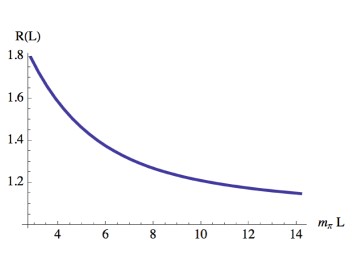
Figure 2: Plot of the ratio $R(L)$ in Eq. (39) as a function of $m_{\pi}L$.

Let us assume that the lattice practitioner has determined the isovector current utilizing the smallest non-vanishing momentum mode, $q=2\pi/L$. Consider the magnetic moment correction as a correction to the finite volume current rather than just narrowly to the magnetic moment. For large enough box size, the smallest momentum mode approaches zero, and so we expect ${\delta}F_{2}^{(I)}(0,L)$ to give a good description of the volume dependence of the finite volume form factor evaluated at the lowest mode. We can address this numerically by comparing ${\delta}F_{2}^{(I)}(0,L)$ to the momentum transfer dependent volume effect. For ease let us assume the lattice kinematics are such that we arrive at Eq. (LABEL:eq:start) in finite volume. We plot the ratio $R(L)$ defined by

$$R(L)=\frac{{\delta}F_{2}^{(I)}(0,L)}{{\delta}F_{2}^{(I)}(q,L)},$$ (39)

as a function of the box size $m_{\pi}L$. This is done in Figure 2. Here $q$ is fixed at the first non-vanishing momentum, and we use the values $g_{A}=1.25$, $|g_{{\Delta}N}|=1.5$, $M_{N}=0.94\,\texttt{GeV}$, and $m_{\pi}/\Delta=0.48$. From the figure, we see that ${\delta}F_{2}^{(I)}(0,L)$ gives a rough estimate of the volume effect for the matrix element under the simplifying kinematical choices. The agreement improves as the box size $L$ increases. The ratio $R(L)$ tends to one asymptotically but only very slowly. Numerically one can see this asymptotic approach set in at $m_{\pi}L\approx 90$. As explained in Hu et al. (2007b), the current matrix element depends on two combinations involving the momentum transfer: $q^{2}/m_{\pi}^{2}$, and $\bm{q}^{2}L^{2}$. For the lowest non-vanishing mode, the latter combination is constant and a series expansion is poorly convergent.

An expansion in $q^{2}/m_{\pi}^{2}$ for large $L$ is well behaved, and we can obtain a different approximation to ${\delta}F_{2}^{(I)}(q,L)$ in the asymptotic regime. It is best to illustrate the issue by considering a similar but simpler example. Notice that for large $m_{\pi}L$,

$$P_{\pi}(x,q^{2})\overset{L\to\infty}{\longrightarrow}1.$$ (40)

Thus a typical finite volume contribution of the form

$$\int_{0}^{1}dx\,I_{\beta}\left(\frac{2\pi nx}{L}\hat{\bm{x}},m_{\pi}P_{\pi}(x,q^{2}),{\Delta}\right)\longrightarrow\int_{0}^{1}dx\,I_{\beta}\left(\frac{2\pi nx}{L}\hat{\bm{x}},m_{\pi},{\Delta}\right),$$ (41)

where we have specified the $n$-th mode in order to track the problematic term. In this limit, the $x$-integral can now be performed because the only $x$-dependence enters in one of the elliptic-theta functions $\vartheta_{3}$, namely as

$$\int_{0}^{1}dx\,\vartheta_{3}(\pi nx,e^{-\tau})=1.$$ (42)

Thus to take the large $L$ limit of $I_{\beta}$, we merely drop the elliptic-theta function in the direction corresponding to the momentum transfer. The resultant volume correction is effectively two dimensional. This procedure is only valid when the momentum transfer is aligned with one of the spatial axes. The generally oriented case is considerably more complicated but the $x$-integration can still be performed. Expanding in $q^{2}/m_{\pi}^{2}$ but not in $\bm{q}^{2}L^{2}$, we arrive at

$${\delta}\tilde{F}_{2}^{(I)}(0,L)=-\frac{6M_{N}}{f^{2}}\int_{0}^{1}dx\left\{g_{A}^{2}I^{22}_{5/2}[xq\hat{\bm{x}},m_{\pi},0]+\frac{2}{9}g_{{\Delta}N}^{2}I^{22}_{5/2}[xq\hat{\bm{x}},m_{\pi},{\Delta}]\right\},$$ (43)

where we have explained above how the $x$-integrals are to be performed analytically. From this correction, we can form the ratio $\tilde{R}(L)={\delta}\tilde{F}_{2}^{(I)}(0,L)/{\delta}F_{2}^{(I)}(q,L)$. This ratio has the same behavior as $R(L)$ shown in Figure 2. The only difference is that $\tilde{R}(L)$ is $\sim 10\%$ larger. The careful expansion leading to ${\delta}\tilde{F}_{2}^{(I)}(0,L)$ thus actually does worse to describe the finite volume matrix element than the naive expansion, ${\delta}F_{2}^{(I)}(0,L)$. The asymptotic approach to unity also sets in for $\tilde{R}(L)$ at $m_{\pi}L\approx 90$. Of course at these volumes any effect is negligible. To compare these approximations to the finite volume matrix element, we plot each individually as a function of $m_{\pi}L$ in Figure 3.

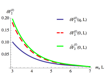
Figure 3: Plot of the finite volume modifications at $\bm{q}=\frac{2\pi}{L}(1,0,0)$. The finite volume matrix element ${\delta}F_{2}^{(I)}(q,L)$, the naive guess ${\delta}F_{2}^{(I)}(0,L)$, and the approximation ${\delta}\tilde{F}_{2}^{(I)}(0,L)$ are plotted as a function of $m_{\pi}L$.

For all practical purposes, beyond $m_{\pi}L\approx 5$ both approximations give reasonable values for the finite volume correction to the current matrix element.

If the simplifying choice of lattice kinematics is not made, the correction ${\delta}F_{2}^{(I)}(0,L)$ ceases to give a good estimate for the volume corrections to the current. We can investigate this by choosing the momentum transfer to be $\bm{q}^{\prime}=\frac{2\pi}{L}(1,1,0)$ and returning to Eq. (28) to determine the volume effect. This effect we denote by ${\delta}F_{2}^{(I)}(q^{\prime},L)$ which has the form

$${\delta}F_{2}^{(I)}(q^{\prime},L) \equiv \frac{LM_{N}}{2\pi i}\Big{[}{\delta}\langle N(\bm{q}^{\prime})\downarrow|\hat{\bm{y}}\cdot\bm{J}_{\text{Iso}}|N(\bm{0})\downarrow\rangle_{L}-{\delta}\langle N(\bm{q}^{\prime})\uparrow|\hat{\bm{y}}\cdot\bm{J}_{\text{Iso}}|N(\bm{0})\uparrow\rangle_{L}\Big{]}$$

$$= -\frac{3M_{N}}{f^{2}}\Bigg{\{}g_{A}^{2}\left[f^{22}(q^{\prime 2},\bm{q}^{\prime},0)-f^{21}(q^{\prime 2},\bm{q}^{\prime},0)\right]+\frac{2}{9}g_{{\Delta}N}^{2}\left[f^{22}(q^{\prime 2},\bm{q}^{\prime},{\Delta})-f^{21}(q^{\prime 2},\bm{q}^{\prime},{\Delta})\right]\Bigg{\}}.$$

Notice we have scaled the matrix elements by a factor of $2\pi/L$, not by $|\bm{q}^{\prime}|$. This is because the overall momentum factor in the matrix element is $2\pi/L$ by virtue of Eqs. (21) and (28). Expanding in large $m_{\pi}L$ but fixed $\bm{q}^{\prime 2}L^{2}$, we can derive the asymptotics of ${\delta}F_{2}^{(I)}(q^{\prime},L)$, which we denote by the function ${\delta}\tilde{F}_{2}^{(I)}(0^{\prime},L)$ and is given by

$${\delta}\tilde{F}_{2}^{(I)}(0^{\prime},L)={\delta}F_{2}^{(I)}(q^{\prime},L)\Bigg{|}_{P_{\pi}(x,q^{\prime 2})=1}.$$ (45)

The resulting $x$-integrals in ${\delta}\tilde{F}_{2}^{(I)}(0^{\prime},L)$ involve products of two $x$-dependent Jacobi elliptic-theta functions. These can be evaluated analytically as shown in Appendix A. The notation $0^{\prime}$ reflects that the asymptotic form still depends on the mode numbers (in this case $n_{x}=n_{y}=1$). We can now compare finite volume effects in the current matrix element for the momentum $\bm{q}^{\prime}=\frac{2\pi}{L}(1,1,0)$. The exact correction ${\delta}F_{2}^{(I)}(q^{\prime},L)$, naive expansion ${\delta}F_{2}^{(I)}(0,L)$, and asymptotic correction ${\delta}\tilde{F}_{2}^{(I)}(0^{\prime},L)$ are each plotted as a function of $m_{\pi}L$ in Figure 4.

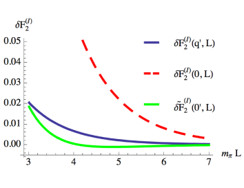
Figure 4: Plot of the finite volume modifications at the momentum transfer $\bm{q}^{\prime}=\frac{2\pi}{L}(1,1,0)$. The finite volume form factor ${\delta}F_{2}^{(I)}(q^{\prime},L)$, the naive expansion ${\delta}F_{2}^{(I)}(0,L)$, and the asymptotic approximation ${\delta}\tilde{F}_{2}^{(I)}(0^{\prime},L)$, are plotted as a function of $m_{\pi}L$.

From the figure we see that naive guess ${\delta}F_{2}^{(I)}(0,L)$ ceases to give a good description of the volume effect. The asymptotic formula ${\delta}\tilde{F}_{2}^{(I)}(0^{\prime},L)$ approaches ${\delta}F_{2}^{(I)}(q^{\prime},L)$ for reasonably large values of $m_{\pi}L$ as it should. There is a crossover for $m_{\pi}L\approx 3$ which is why the curves start out in near agreement on the plot.

Now we remind the reader that ${\delta}F_{2}^{(I)}(0,L)$ was derived as the finite volume modification to the magnetic moment, which we denote ${\delta}\mu_{N}^{(I)}(L)$. Above we have been considering this term as a correction to the finite volume form factors. The question remains: if we use lattice data for the current matrix element, to what extent is the finite volume correction to the magnetic moment described by ${\delta}\mu_{N}^{(I)}(L)$? Based on our discussion leading up to Eq. (38), we expect a poor description of the volume effect with current lattice sizes. We can only describe the behavior qualitatively because it depends on precisely how the magnetic moment is extracted from the lattice data.

Generally speaking what happens in any procedure (including modeling the momentum transfer dependence) is some type of weighting over the values of the current matrix element for the smallest momentum modes. The simplest way to do this is to take the slope of the current matrix elements for the two smallest non-vanishing momenta. By Eq. (21), the slope should be the magnetic moment. Now consider the volume corrections to the current matrix element at each of the sampled momenta. For nearby modes, the volume effect has a good degree of cancellation and is hence reduced. Compare this to ${\delta}F_{2}^{(I)}(0,L)$ which provides an otherwise decent estimate of either of the individual values of the current matrix element, and consequently a poor estimate of their difference. We expect this argument to qualitatively generalize when one considers an arbitrary weighting of contributions from small momentum modes. This constitutes a rough description of how one models the momentum transfer dependence of form factors.

The safest route in dealing with volume corrections is to deduce them for the momentum modes at which the current has been calculated. Use the effective theory, if possible, to isolate the infinite volume values of the form factor at these data points, then perform a momentum extrapolation to extract the infinite volume magnetic moment. Carrying out the procedure in the opposite order most likely leads to specious volume dependence.

IV.3 Form Factor Puzzle

Finally we explore a surprising consequence of our finite volume expressions for current matrix elements. We show that values of current matrix elements calculated at two different momenta sharing the same value of momentum transfer squared generally differ. This puzzling feature is a manifestation of the lack of rotational invariance in lattice data.

We consider volume corrections to the isovector Pauli form factor and thus return to the general expression in Eq. (28). Above we have determined the effect of the finite volume at $\bm{q}^{\prime}=\frac{2\pi}{L}(1,1,0)$. Now we additionally determine the effect at the momentum $\bm{q}^{\prime\prime}=\frac{2\pi}{L}(1,0,1)$. Of course $\bm{q}^{\prime 2}=\bm{q}^{\prime\prime 2}$, and in infinite volume the form factor must be the same by rotational invariance. For both momenta, we utilize the $y$-component of the current.

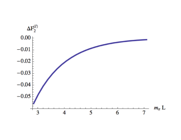
Figure 5: Plot of the form factor difference ${\Delta}F_{2}^{(I)}=F_{2}^{(I)}(\bm{q}^{\prime 2})-F_{2}^{(I)}(\bm{q}^{\prime\prime 2})$, with $\bm{q}^{\prime 2}=\bm{q}^{\prime\prime 2}=8\pi^{2}/L^{2}$, as a function of $m_{\pi}L$. Rotational invariance at infinite volume requires this difference to vanish.

To compare the value of the form factor at these differing momenta, we form the difference ${\Delta}F_{2}^{(I)}$ given by

$${\Delta}F_{2}^{(I)} = \frac{LM_{N}}{2\pi i}\Big{[}\langle N(\bm{q}^{\prime})\downarrow|\hat{\bm{y}}\cdot\bm{J}_{\text{Iso}}|N(\bm{0})\downarrow\rangle_{L}-\langle N(\bm{q}^{\prime})\uparrow|\hat{\bm{y}}\cdot\bm{J}_{\text{Iso}}|N(\bm{0})\uparrow\rangle_{L}\Big{]}$$ (46)

$$-\frac{LM_{N}}{2\pi i}\Big{[}\langle N(\bm{q}^{\prime\prime})\downarrow|\hat{\bm{y}}\cdot\bm{J}_{\text{Iso}}|N(\bm{0})\downarrow\rangle_{L}-\langle N(\bm{q}^{\prime\prime})\uparrow|\hat{\bm{y}}\cdot\bm{J}_{\text{Iso}}|N(\bm{0})\uparrow\rangle_{L}\Big{]}.$$

Accordingly the infinite volume pieces of the current matrix elements cancel out of ${\Delta}F_{2}^{(I)}$. Thus ${\Delta}F_{2}^{(I)}$ gives a measure of how much calculations of the form factor at $\bm{q}^{\prime 2}=\frac{8\pi^{2}}{L^{2}}$ and $\bm{q}^{\prime\prime 2}=\frac{8\pi^{2}}{L^{2}}$ differ. Using the expression for the volume effect, Eq. (28), as well as expressions from Appendix A, we determine ${\Delta}F_{2}^{(I)}$ to be

$${\Delta}F_{2}^{(I)}=-\frac{6M_{N}}{f^{2}}\left[g_{A}^{2}f(0)+\frac{2}{9}g_{{\Delta}N}^{2}f({\Delta})\right],$$ (47)

where the function $f({\Delta})$ is given by

$$f({\Delta}) = \frac{1}{24\pi^{3/2}L}\int_{0}^{1}dx\int_{0}^{\infty}d\tau\sqrt{\tau}e^{-(m_{\pi}^{2}P_{\pi}(x,q^{\prime 2})^{2}-{\Delta}^{2})L^{2}/4\tau}\operatorname{Erfc}\left(\frac{{\Delta}L}{2\sqrt{\tau}}\right)$$

$$\times\left[\vartheta^{\prime\prime}_{3}(\pi x,e^{-\tau})\vartheta_{3}(\pi x,e^{-\tau})\vartheta_{3}(0,e^{-\tau})-\vartheta^{\prime}_{3}(\pi x,e^{-\tau})^{2}\vartheta_{3}(0,e^{-\tau})-\vartheta^{\prime\prime}_{3}(0,e^{-\tau})\vartheta_{3}(\pi x,e^{-\tau})^{2}\right].$$

We plot ${\Delta}F_{2}^{(I)}$ in Figure 5, and indeed find that the finite volume form factor does not respect rotational invariance. From the Figure, moreover, we see that for asymptotically large volumes rotational invariance is restored. This can easily be demonstrated analytically from Eq. (LABEL:eq:mixedup). This is a general feature of finite volume form factors. One can easily verify the lack of rotational invariance for the isoscalar combination as well as charge form factor, for example.

The fact that different momenta (which share the same magnitude) yield differing current matrix elements is already evident from the general structure of the finite volume effective action, Eq. (7) [as well as Eq. (60) in Appendix B]. The new couplings allowed on a torus break rotational invariance. While these couplings vanish at one-loop order in heavy baryon $\chi$PT, there are indeed non-vanishing couplings at higher orders in the derivative expansion. These terms are not suppressed, however, because all terms in the derivative expansion in powers of $\bm{q}^{2}L^{2}$ are order one.

In confronting actual lattice data for current matrix elements, we cannot attribute all differences at identical momentum transfer squared to volume effects. The discretization also breaks rotational invariance. Thus at infinite volume but finite lattice spacing, matrix elements are only hypercubic invariant functions of the momentum. Generally differences seen in lattice form factor data arise from the violation of rotational invariance from both volume and discretization effects. Physically one expects the dominant source of difference to be from the volume (discretization) at small (large) momentum transfer.

V Summary

Above we have analyzed the finite volume current matrix elements of the nucleon. Focusing specifically on the isovector contribution, we have deduced in Eq. (28) the finite volume correction to lattice calculations of the electromagnetic three-point function. This finite volume result does not have an interpretation as a correction to the Pauli form factor. A decomposition of matrix elements in terms of Dirac and Pauli form factors makes use of Lorentz and gauge invariance. The former is not relevant for a torus, while the latter has new features in finite volume due to the special gauge transformation of the zero-mode.

For the smallest available momentum transfer on the lattice, $q=2\pi/L$, we have shown numerically that one cannot series expand finite volume results in powers of the photon momentum. This result applies generally, not just to current matrix elements. Consider a simple Feynman diagram with momentum insertion in finite volume. Using a Feynman parameter to combine denominators, the typical contribution has the form

$$\propto\int_{0}^{1}dx\sum_{\bm{n}}\left[4\pi^{2}(\bm{n}+x\bm{m})^{2}+(m_{\pi}L)^{2}\left(1-x(1-x)\frac{q^{2}}{m_{\pi}^{2}}\right)\right]^{-{\beta}},$$ (49)

where $\bm{q}=2\pi\bm{m}/L$ is the inserted momentum. In infinite volume, multipole expansions are well defined in terms of the expansion parameter ${\lambda}=q^{2}/m_{\pi}^{2}$. In finite volume, this expansion remains well behaved, ${\lambda}\propto(m_{\pi}L)^{-2}$ for large $L$. There are additional finite volume terms, however, that depend on the combination $\bm{q}^{2}L^{2}=4\pi^{2}\bm{m}^{2}$. Such dependence cannot be expanded out even in large volumes. Thus working at only the smallest momentum transfer, we cannot deduce volume corrections to multipole moments, cf Figure 2. The approximate agreement shown in the figure results from simplifying assumptions about the lattice kinematics used to measure the current. The agreement worsens when such choices are not made, see Figure 4.

On the other hand, for large enough momenta the relative spacing between modes becomes small enough to approximate a derivative. In this regime, one can series expand finite volume modifications as has been done in the literature. The resulting frequency expansion is not a multipole expansion, however, but is described by a theory of Wilson lines, as in Eq. (7). New couplings are allowed and lead to current screening, for example. For the isovector magnetic moment of the nucleon, we showed that a new zero-mode coupling allowed by symmetry vanishes at next-to-leading order in heavy baryon chiral perturbation theory. Consequently we were able to recover previously derived results Beane (2004). In order for such results to be valid, however, one requires momenta small enough for the efficacy of a low-energy effective theory, and at the same time large enough in order to treat the momentum as continuous. Satisfying such restrictions is considerably beyond the reach of current computing power. In practice, one must retain the momentum transfer dependence of finite volume matrix elements to account for the volume effect in lattice correlation functions. Finally we showed that such finite volume corrections to form factors can lead to surprising effects. Specifically current matrix elements evaluated at identical $\bm{q}^{2}$, but differing $\bm{q}$, need not be the same.

Appendix A Glossary of Finite Volume Functions

Above we have determined the finite volume modifications to single nucleon current matrix elements. In this Appendix, we give explicit formulae for the finite volume difference functions used in the main text. We use similar notation for these functions as Sachrajda and Villadoro (2005); Tiburzi (2006), where further discussion can be found.

In evaluating a Feynman diagram in finite volume, the loops contain a sum over the allowed Fourier modes in a periodic box. The difference of this sum and the infinite volume integral is the finite volume effect. As is customary, we treat the length of the time direction as infinite. In a heavy fermion formulation, all finite volume differences with momentum insertion can be cast in terms of the function $I_{\beta}^{i_{1}\cdots i_{j}}(\bm{\theta},m,{\delta})$, defined by

$$I^{i_{1}\cdots i_{j}}_{\beta}(\bm{\theta},m,{\delta}) = \int_{0}^{\infty}d{\lambda}\left\{\frac{1}{L^{3}}\sum_{\bm{n}}\frac{q^{i_{1}}\cdots q^{i_{j}}}{[(\bm{q}+\bm{\theta})^{2}+m^{2}+2{\delta}{\lambda}+{\lambda}^{2}]^{\beta}}\right.$$ (50)

$$\phantom{spaceforspace}\left.-\int\frac{d\bm{q}}{(2\pi)^{3}}\frac{q^{i_{1}}\cdots q^{i_{j}}}{[(\bm{q}+\bm{\theta})^{2}+m^{2}+2{\delta}{\lambda}+{\lambda}^{2}]^{\beta}}\right\},$$

where $\bm{n}$ sums over triplets of integers, and the momentum modes satisfy the periodic box quantization condition, $\bm{q}=2\pi\bm{n}/L$. While general expressions for the exponentially convergent form of $I_{\beta}^{i_{1}\cdots i_{j}}(\bm{\theta},m,{\delta})$ exist, we merely cite the required cases for our work. These are

$$I_{\beta}(\bm{\theta},m,{\delta}) = \frac{(L/2)^{2{\beta}}}{\pi L^{4}\Gamma(\beta)}\int_{0}^{\infty}d\tau\,\tau^{1-{\beta}}e^{-(m^{2}-{\delta}^{2})L^{2}/4\tau}\operatorname{Erfc}\left(\frac{{\delta}L}{2\sqrt{\tau}}\right)\left[\prod_{j=1}^{3}\vartheta_{3}(\theta_{j}L/2,e^{-\tau})-1\right],$$

$$I_{\beta}^{i_{1}}(\bm{\theta},m,{\delta}) = -\frac{1}{2({\beta}-1)}\frac{d}{d\theta^{i_{1}}}I_{{\beta}-1}(\bm{\theta},m,{\delta})-\theta^{i_{1}}I_{\beta}(\bm{\theta},m,{\delta}),\,\text{and}$$ (52)

$$I_{\beta}^{i_{1}i_{2}}(\bm{\theta},m,{\delta}) = \frac{1}{4({\beta}-2)({\beta}-1)}\frac{d^{2}}{d\theta^{i_{1}}d\theta^{i_{2}}}I_{{\beta}-2}(\bm{\theta},m,{\delta})+\frac{1}{2({\beta}-1)}{\delta}^{i_{1}i_{2}}I_{{\beta}-1}(\bm{\theta},m,{\delta})$$

$$+\frac{1}{2({\beta}-1)}\left[\theta^{i_{1}}\frac{d}{d{\theta}^{i_{2}}}I_{{\beta}-1}(\bm{\theta},m,{\delta})+\theta^{i_{2}}\frac{d}{d{\theta}^{i_{1}}}I_{{\beta}-1}(\bm{\theta},m,{\delta})\right]+\theta^{i_{1}}\theta^{i_{2}}I_{\beta}(\bm{\theta},m,{\delta}),$$

where $\vartheta_{3}(z,q)$ is the Jacobi elliptic-theta function of the third kind, and $\operatorname{Erfc}(z)$ is the complement of the standard error function. The finite volume physics arising from the mass splitting parameter ${\delta}$ is well explicated in Arndt and Lin (2004).

In expanding matrix elements about zero external momentum, one also has use for the functions $J_{\beta}(m,{\delta})$, and $K_{\beta}(m,{\delta})$ given by

$$J_{\beta}(m,{\delta}) = -\frac{1}{4({\beta}-1)({\beta}-2)}\frac{\partial^{2}}{\partial{\delta}^{2}}I_{{\beta}-2}(\bm{0},m,{\delta})+\left(1+\frac{{\delta}}{{\beta}-1}\frac{\partial}{\partial{\delta}}\right)I_{{\beta}-1}(\bm{0},m,{\delta})-m^{2}I_{{\beta}}(\bm{0},m,{\delta}),$$

$$K_{\beta}(m,{\delta}) = -\frac{1}{4({\beta}-1)({\beta}-2)}\frac{\partial^{2}}{\partial{\delta}^{2}}J_{{\beta}-2}(\bm{0},m,{\delta})+\left(1+\frac{{\delta}}{{\beta}-1}\frac{\partial}{\partial{\delta}}\right)J_{{\beta}-1}(\bm{0},m,{\delta})-m^{2}J_{{\beta}}(\bm{0},m,{\delta}).$$

Lastly of use are Feynman parameter integrals of Jacobi elliptic-theta functions.

$$\int_{0}^{1}dx\,\vartheta_{3}(\pi x,q)=1,$$ (56)

$$\int_{0}^{1}dx\,\vartheta_{3}(\pi x,q)^{2}=\vartheta_{3}(0,q^{2}),$$ (57)

$$\int_{0}^{1}dx\,\vartheta^{\prime}_{3}(\pi x,q)^{2}=-\vartheta^{\prime\prime}_{3}(0,q^{2}),$$ (58)

$$\int_{0}^{1}dx\,\vartheta^{\prime\prime}_{3}(\pi x,q)\vartheta_{3}(\pi x,q)=\vartheta^{\prime\prime}_{3}(0,q^{2}).$$ (59)

Here the primes denote derivatives with respect to the first argument. Double primes can be traded in for single derivatives with respect to the second argument because the $\vartheta_{3}(z,q)$ satisfy a diffusion equation.

Appendix B Magnetic Radius

In this Appendix, we present the extension of the finite volume effective action in Eq. (7) to higher order in the derivative expansion. This will allow us to consider the finite volume corrections to the magnetic radius. For simplicity, we ignore the charge radius and focus just on the spin-dependent part of the single particle effective action.

Using the cubic symmetry of the torus, it is easy to see that there are no spin-dependent terms with two derivatives. Including all spin-dependent terms with three derivatives and at most one insertion of ${\mathcal{W}}_{i}^{(-)}$, we arrive at the nucleon effective action

$${\mathcal{L}} = {\overline{N}}\Big{[}C_{3}(L)\bm{\sigma}\cdot\partial^{2}\bm{B}-C_{4}(L)\bm{\sigma}\cdot\nabla^{2}\bm{B}-C_{5}(L)\bm{\sigma}\cdot(\bm{\nabla}\times\nabla^{2}\bm{{\mathcal{W}}}^{(-)})$$ (60)

$$-C_{6}(L)\sum_{i}\sigma_{i}\nabla_{i}\nabla_{i}B_{i}-C_{7}(L)\sum_{i}\varepsilon_{ijk}\sigma_{i}\nabla_{i}\nabla_{i}\nabla_{j}{\mathcal{W}}^{(-)}_{k}\Big{]}N.$$

Here the couplings $C_{4}(L)$, $C_{5}(L)$, $C_{6}(L)$, and $C_{7}(L)$ run to zero as the volume goes to infinity. This reflects that the corresponding operators are forbidden by infinite volume gauge invariance, and Lorentz invariance. The remaining coupling $C_{3}(L)$, satisfies

$$C_{3}(L)=C_{3}+\delta C_{3}(L),$$ (61)

where $C_{3}$ is the infinite volume coupling given by

$$C_{3}=6<r_{M}^{2}>,$$ (62)

with $<r_{M}^{2}>$ as the mean-square magnetic radius which we define by $-\frac{1}{6}\frac{d}{dq^{2}}F_{2}(q^{2})$. The finite volume effect $6\,{\delta}C_{3}(L)$ is thus the correction to the magnetic radius, however, there are four additional operators that also make contributions to spin polarized current matrix elements in finite volume.

To determine the couplings in Eq. (60), we turn to heavy baryon chiral perturabtion theory. Specifically we need the result derived above for spin polarized current matrix elements, Eq. (28). We expand this result to third order in the photon frequency and match onto Eq. (60). This will determine the isovector part of the coupling constants. We find

$$\delta C_{3}(L) = \frac{5}{6f^{2}}\left[g_{A}^{2}J_{7/2}(m_{\pi},0)+\frac{2}{9}J_{7/2}(m_{\pi},{\Delta})\right],$$

$$C_{4}(L) = \frac{1}{3f^{2}}\left[g_{A}^{2}\left(7K_{9/2}(m_{\pi},0)-5J_{7/2}(m_{\pi},0)\right)+\frac{2}{9}g_{{\Delta}N}^{2}\left(7K_{9/2}(m_{\pi},{\Delta})-5J_{7/2}(m_{\pi},{\Delta})\right)\right],$$

$$C_{5}(L) = C_{6}(L)=C_{7}(L)=0.$$ (63)

The finite volume functions $J_{\beta}(m,{\delta})$ and $K_{\beta}(m,{\delta})$ are defined in Appendix A. The fact that $C_{3}(L)$ and $C_{4}(L)$ are non-vanishing to this order means that it is not possible to define the magnetic radius at finite volume. The remaining coefficients require further terms in the chiral expansion to be non-vanishing. The non-relativistic nature of the nucleon in heavy baryon chiral perturbation theory is likely the culprit for the vanishing of these terms at next-to-leading order. In the meson sector, by contrast, derivative couplings lead to a myriad of new finite volume terms, see Hu et al. (2007b).

References

- DeGrand and DeTar (2006) T. DeGrand and C. DeTar, Lattice Methods for Quantum Chromodynamics (World Scientific, 2006).
- Gasser and Leutwyler (1987a) J. Gasser and H. Leutwyler, Phys. Lett. B184, 83 (1987a).
- Gasser and Leutwyler (1987b) J. Gasser and H. Leutwyler, Phys. Lett. B188, 477 (1987b).
- Gasser and Leutwyler (1988) J. Gasser and H. Leutwyler, Nucl. Phys. B307, 763 (1988).
- Leutwyler (1987) H. Leutwyler, Phys. Lett. B189, 197 (1987).
- Luscher (1991a) M. Luscher, Nucl. Phys. B364, 237 (1991a).
- Luscher (1991b) M. Luscher, Nucl. Phys. B354, 531 (1991b).
- Lellouch and Luscher (2001) L. Lellouch and M. Luscher, Commun. Math. Phys. 219, 31 (2001), eprint hep-lat/0003023.
- Beane (2004) S. R. Beane, Phys. Rev. D70, 034507 (2004), eprint hep-lat/0403015.
- Arndt and Lin (2004) D. Arndt and C. J. D. Lin, Phys. Rev. D70, 014503 (2004), eprint hep-lat/0403012.
- Beane and Savage (2004) S. R. Beane and M. J. Savage, Phys. Rev. D70, 074029 (2004), eprint hep-ph/0404131.
- Bernard et al. (2007) V. Bernard, U.-G. Meissner, and A. Rusetsky (2007), eprint hep-lat/0702012.
- Ali Khan et al. (2004) A. Ali Khan et al. (QCDSF-UKQCD), Nucl. Phys. B689, 175 (2004), eprint hep-lat/0312030.
- Colangelo and Haefeli (2004) G. Colangelo and C. Haefeli, Phys. Lett. B590, 258 (2004), eprint hep-lat/0403025.
- Colangelo et al. (2005) G. Colangelo, S. Durr, and C. Haefeli, Nucl. Phys. B721, 136 (2005), eprint hep-lat/0503014.
- Colangelo and Haefeli (2006) G. Colangelo and C. Haefeli, Nucl. Phys. B744, 14 (2006), eprint hep-lat/0602017.
- Detmold and Savage (2004) W. Detmold and M. J. Savage, Phys. Lett. B599, 32 (2004), eprint hep-lat/0407008.
- Bedaque et al. (2005) P. F. Bedaque, H. W. Griesshammer, and G. Rupak, Phys. Rev. D71, 054015 (2005), eprint hep-lat/0407009.
- Smigielski and Wasem (2007) B. Smigielski and J. Wasem (2007), eprint arXiv:0706.3731 [hep-lat].
- Beane et al. (2004) S. R. Beane, P. F. Bedaque, A. Parreno, and M. J. Savage, Phys. Lett. B585, 106 (2004), eprint hep-lat/0312004.
- Bedaque et al. (2006) P. F. Bedaque, I. Sato, and A. Walker-Loud, Phys. Rev. D73, 074501 (2006), eprint hep-lat/0601033.
- Sato and Bedaque (2007) I. Sato and P. F. Bedaque, Phys. Rev. D76, 034502 (2007), eprint hep-lat/0702021.
- Beane et al. (2007) S. R. Beane, W. Detmold, and M. J. Savage (2007), eprint arXiv:0707.1670 [hep-lat].
- Detmold and Lin (2005) W. Detmold and C. J. D. Lin, Phys. Rev. D71, 054510 (2005), eprint hep-lat/0501007.
- Bunton et al. (2006) T. B. Bunton, F. J. Jiang, and B. C. Tiburzi, Phys. Rev. D74, 034514 (2006), eprint hep-lat/0607001.
- Chen et al. (2007) J.-W. Chen, W. Detmold, and B. Smigielski, Phys. Rev. D75, 074003 (2007), eprint hep-lat/0612027.
- Detmold et al. (2006) W. Detmold, B. C. Tiburzi, and A. Walker-Loud, Phys. Rev. D73, 114505 (2006), eprint hep-lat/0603026.
- Hu et al. (2007a) J. Hu, F.-J. Jiang, and B. C. Tiburzi, Phys. Lett. B653, 350 (2007a), eprint arXiv:0706.3408 [hep-lat].
- Hu et al. (2007b) J. Hu, F.-J. Jiang, and B. C. Tiburzi (2007b), eprint arXiv:0709.1955 [hep-lat].
- Martinelli et al. (1982) G. Martinelli, G. Parisi, R. Petronzio, and F. Rapuano, Phys. Lett. B116, 434 (1982).
- Bernard et al. (1982) C. W. Bernard, T. Draper, K. Olynyk, and M. Rushton, Phys. Rev. Lett. 49, 1076 (1982).
- Lee et al. (2005) F. X. Lee, R. Kelly, L. Zhou, and W. Wilcox, Phys. Lett. B627, 71 (2005), eprint hep-lat/0509067.
- Jenkins and Manohar (1991) E. Jenkins and A. V. Manohar, Phys. Lett. B255, 558 (1991).
- Luke and Manohar (1992) M. E. Luke and A. V. Manohar, Phys. Lett. B286, 348 (1992), eprint hep-ph/9205228.
- Zinn-Justin (1996) J. Zinn-Justin, Int. Ser. Monogr. Phys. 92, 1 (1996).
- Jenkins et al. (1993) E. E. Jenkins, M. E. Luke, A. V. Manohar, and M. J. Savage, Phys. Lett. B302, 482 (1993), eprint hep-ph/9212226.
- Bernard et al. (1992) V. Bernard, N. Kaiser, J. Kambor, and U. G. Meissner, Nucl. Phys. B388, 315 (1992).
- Bernard et al. (1998) V. Bernard, H. W. Fearing, T. R. Hemmert, and U. G. Meissner, Nucl. Phys. A635, 121 (1998), eprint hep-ph/9801297.
- Sachrajda and Villadoro (2005) C. T. Sachrajda and G. Villadoro, Phys. Lett. B609, 73 (2005), eprint hep-lat/0411033.
- Tiburzi (2006) B. C. Tiburzi, Phys. Lett. B641, 342 (2006), eprint hep-lat/0607019.