Stationary probability density of stochastic search processes in global optimization

Abstract

A method for the construction of approximate analytical expressions for the stationary marginal densities of general stochastic search processes is proposed. By the marginal densities, regions of the search space that with high probability contain the global optima can be readily defined. The density estimation procedure involves a controlled number of linear operations, with a computational cost per iteration that grows linearly with problem size.

Keywords: Stochastic search, Heuristics

1 Diffusion and Global Optimization

Stochastic strategies for optimization are essential to many of the heuristic techniques used to deal with complex, unstructured global optimization problems. Methods like simulated annealing [1, 2, 3, 4] and evolutionary algorithms [5, 6, 7], have proven to be valuable tools, capable of give good quality solutions at a relatively small computational effort. In spite of their success, these approaches present a major drawback, namely the absence of valid bounds on the obtained solutions. A common feature of deterministic global optimization algorithms is the progressive reduction of the domain space until the global optimum has been found with arbitrary accuracy [8, 9]. An analogous property for stochastic algorithms has been largely lacking. In this contribution is introduced a method for the estimation of the asymptotic probability density of a general stochastic search process in global optimization problems. The convergence of the estimated density can be clearly assessed, and with the help of this density, reliable bounds for the location of the global optimum are derived. The procedure involves linear operations only, and a well defined number of evaluations of the given cost function. The presented results indicate that by the proposed approach, regions of the search space can be discarded on a probabilistic basis. This property may be implemented in a variety of ways in order to improve existing or develop new optimization algorithms, and open the door for the construction of probabilistic optimality certificates in large scale nonlinear optimization problems.

The roots of stochastic search methods can be traced back to the Metropolis algorithm [10], introduced in the early days of scientific computing to simulate the evolution of a physical system to thermal equilibrium. This process is the base of the simulated annealing technique [1], which makes use of the convergence to a global minimum in configurational energy observed in physical systems at thermal equilibrium as the temperature goes to zero. The method presented in this contribution is rooted in similar physical principles as those on which simulated annealing and related algorithms [1, 11, 2, 3] are based. However, in contrast with other approaches, the proposed method considers a density of points instead of Markov transitions of individual points. Moreover, the main goal of the proposed approach is not the convergence to global minima as a randomness parameter is reduced, but the approximation of the probability density after an infinitely long exploration time of the search space, keeping a fixed randomness.

Consider the minimization of a cost function of the form $V(x_{1},x_{2},...,x_{n},...,x_{N})$ with a search space defined over $L_{1,n}\leq x_{n}\leq L_{2,n}$. A stochastic search process for this problem is modeled by

$$\dot{x}_{n}=-\frac{\partial V}{\partial x_{n}}+\varepsilon(t),$$ (1)

where $\varepsilon(t)$ is an additive noise with zero mean. Equation (1), known as Langevin equation in the Statistical Physics literature [12, 13], captures the basic properties of a general stochastic search strategy. Under an uncorrelated Gaussian noise with constant strength, Eq. (1) represents a search by diffusion, while a noise strength that is slowly varying in time gives a simulated annealing. Notice that when choosing an external noise of infinite amplitude, the dynamical influence of the cost function over the exploration process is lost, leading to a blind search. The model given by Eq.(1) can be also interpreted as an overdamped nonlinear dynamical system composed by $N$ interacting particles. The temporal evolution of the probability density of such a system in the presence of an additive Gaussian white noise, is described by a linear differential equation, the Fokker – Planck equation [12, 13],

$$\dot{p}=\frac{\partial}{\partial x}\left[\frac{\partial V}{\partial x}p\right]+D\frac{\partial^{2}p}{\partial x^{2}}$$ (2)

where $D$ is a constant, called diffusion constant, that is proportional to the noise strength. The direct use of Eq. (2) for optimization or deviate generation purposes would imply the calculation of high dimensional integrals. It results numerically much less demanding to perform the following one dimensional projection of Eq. (2). Under very general conditions (e. g., the absence of infinite cost values), the equation (2) has a stationary solution over a search space with reflecting boundaries [12, 14]. The stationary conditional probability density satisfy the one dimensional Fokker – Planck equation

$$D\frac{\partial p(x_{n}|\{x_{j\neq n}=x_{j}^{*}\})}{\partial x_{n}}+p(x_{n}|\{x_{j\neq n}=x_{j}^{*}\})\frac{\partial V}{\partial x_{n}}=0.$$ (3)

An important consequence of Eq. (3) is that the marginal $p(x_{n})$ can be sampled by drawing points from the conditional $p(x_{n}|\{x_{j\neq n}=x_{j}^{*}\})$ via a Gibbs sampling [15]. It is now shown how, due to the linearity of the Fokker – Planck equation, a particular form of Gibbs sampling can be constructed, such that its not only possible to sample the marginal density, but to give an approximate analytical expression for it. From Eq. (3) follows a linear second order differential equation for the cumulative distribution $y(x_{n}|\{x_{j\neq n}=x_{j}^{*}\})=\int_{-\infty}^{x_{n}}p(x^{{}^{\prime}}_{n}|\{x_{j\neq n}=x_{j}^{*}\})dx^{{}^{\prime}}_{n}$,

$$\frac{d^{2}y}{dx_{n}^{2}}+\frac{1}{D}\frac{\partial V}{\partial x_{n}}\frac{dy}{dx_{n}}=0,$$ (4)

$$y(L_{1,n})=0,\quad y(L_{2,n})=1.$$

Random deviates can be drawn from the density $p(x_{n}|\{x_{j\neq n}=x_{j}^{*}\})$ by the fact that $y$ is an uniformly distributed random variable in the interval $y\in[0,1]$. Viewed as a function of the random variable $x_{n}$, $y(x_{n}|\{x_{j\neq n}\})$ can be approximated through a linear combination of functions from a complete set that satisfy the boundary conditions in the interval of interest,

$$\hat{y}(x_{n}|\{x_{j\neq n}\})=\sum_{l=1}^{L}a_{l}\varphi_{l}(x_{n}).$$ (5)

Choosing for instance, a basis in which $\varphi_{l}(0)=0$, the $L$ coefficients are uniquely defined by the evaluation of Eq. (4) in $L-1$ interior points. In this way, the approximation of $y$ is performed by solving a set of $L$ linear algebraic equations, involving $L-1$ evaluations of the derivative of $V$.

The proposed procedure is based on the iteration of the following steps:

1) Fix the variables $x_{j\neq n}=x_{j}^{*}$ and approximate $y(x_{n}|\{x_{j\neq n}\})$ by the use of formulas (4) and (5).

2) By the use of $\hat{y}(x_{n}|\{x_{j\neq n}\})$ construct a lookup table in order to generate a deviate $x_{n}^{*}$ drawn from the stationary distribution $p(x_{n}|\{x_{j\neq n}=x_{j}^{*}\})$.

3) Update $x_{n}=x_{n}^{*}$ and repeat the procedure for a new variable $x_{j\neq n}$.

The iteration of the three steps above give an algorithm for the estimation of the equilibrium distribution of the stochastic search process described by Eq. (1). A convergent representation for $p(x_{n})$ is obtained after taking the average of the coefficients $a$’s in the expansion (5) over the iterations. In order to see this, consider the expressions for the marginal density and the conditional distribution,

$$p(x_{n})=\int p(x_{n}|\{x_{j\neq n}\})p(\{x_{j\neq n}\})d\{x_{j\neq n}\},$$ (6)

$$y(x_{n}|\{x_{j\neq n}\})=\int_{-\infty}^{x_{n}}p(x^{{}^{\prime}}_{n}|\{x_{j\neq n}\})dx^{{}^{\prime}}_{n}.$$ (7)

From the last two equations follow that the marginal $y(x_{n})$ is given by the expected value of the conditional $y(x_{n}|\{x_{j\neq n}\})$ over the set $\{x_{j\neq n}\}$,

$$y(x_{n})=E_{\{x_{j\neq n}\}}[y(x_{n}|\{x_{j\neq n}\})].$$ (8)

All the information on the set $\{x_{j\neq n}\}$ is stored in the coefficients of the expansion (5). Therefore

$$\left<\hat{y}\right>=\sum_{l=1}^{L}\left<a_{l}\right>\varphi_{l}(x_{n})\to y(x_{n}),$$ (9)

where the brackets represent the average over the iterations of the density estimation procedure.

Previous preliminary applications of the density estimation method on the generation of suitable populations of initial points for optimization algorithms can be found in [16]. In the next section the capabilities of the proposed algorithm for the construction of reliable probabilistic bounds is tested on several benchmark unconstrained examples and in a family of well known constrained NP-hard problems.

2 Examples

The fundamental parameters of the density estimation procedure, $L$ and $D$, have a clear meaning, which is very helpful for their selection. The diffusion constant “smooth” the density. This is evident by taking the limit $D\to\infty$ in Eq. (4), which imply an uniform density in the domain. The number of base functions $L$, on the other hand, defines the algorithms capability to “learn” more or less complicated density structures. Therefore, for a given $D$, the number $L$ should be at least large enough to assure that the estimation algorithm will generate valid distributions $y(x_{n}|\{x_{j\neq n}\})$. A valid distribution should be a monotone increasing continuos function that satisfy the boundary conditions. The parameter $L$ ultimately determines the computational cost of the procedure, because at each iteration a system of size $\propto L$ of linear algebraic equations must be solved $N$ times. Therefore, the user is able to control the computational cost through the interplay of the two basic parameters: for a larger $D$ a smoother density should be estimated, so a lesser $L$ can be used.

The density estimation algorithm is tested on the following benchmark unconstrained problems:

Schwefel:

$$N=6,\quad f=418.9829N-\sum_{n=1}^{N}x_{n}sin(\sqrt{|x_{n}|}),$$

$$-500\leq x_{n}\leq 500,\quad solution:\quad x^{*}=(420.9687,...,420.9687),f(x^{*})=0.$$

Levy No. 5:

$$N=2\quad f=\sum_{i=1}^{5}icos((i-1)x_{1}+i)\sum_{j=1}^{5}jcos((j+1)x_{2}+j)$$

$$+(x_{1}+1.42513)^{2}+(x_{2}+0.80032)^{2},$$

$$-10\leq x_{n}\leq 10,\quad solution:\quad x^{*}=(-1.3068,-1.4248),f(x^{*})=-176.1375.$$

Booth:

$$N=2,\quad f=(x_{1}+2x_{2}-7)^{2}+(2x_{1}+x_{2}-5)^{2},$$

$$-10\leq x_{n}\leq 10,\quad solution:\quad x^{*}=(1,3),f(x^{*})=0.$$

Colville:

$$N=4,\quad f=100(x_{2}-x_{1})^{2}+(1-x_{1})^{2}+90(x_{4}-x_{3})^{2}+(1-x_{3})^{2}$$

$$+10.1((x_{2}-1)^{2}+(x_{4}-1)^{2})+19.8(x_{2}-1)(x_{4}-1),$$

$$-10\leq x_{n}10,\quad solution:\quad x^{*}=(1,...,1),f(x^{*})=0.$$

Rosenbrock:

$$N=20,\quad f=\sum_{n=1}^{N}100(x_{n+1}-x_{n}^{2})^{2}+(x_{n}-1)^{2},$$

$$-10\leq x_{n}\leq 10,\quad solution:\quad x^{*}=(1,...,1),f(x^{*})=0.$$

For the experiments, the following specific form of the expansion (5) has been used,

$$\hat{y}=\sum_{l=1}^{L}a_{l}sin\left((2l-1)\frac{\pi(x_{n}-L_{1,n})}{2(L_{2,n}-L_{1,n})}\right),$$ (10)

so the size of the algebraic system of equations is $L-1$. The linear system has been solved by a LU decomposition routine [17]. The gradients have been calculated numerically, with two cost function evaluations per derivative. In this way, the total number of cost function evaluations per iteration goes like $2(L-1)N$.

In Fig. 1 two different pairs $L,D$ have been considered in the study of the Schwefel problem. This problem has a second best minimum at a relatively large distance of the global optimum. This is reflected on the estimated densities, but at small $D$ a clear distiction between the two regions is made. The Schwefel problem is an example of a separable function, that is, a function given by a linear combination of terms, where each term involves a single variable. Separable problems generate an uncoupled dynamics of the stochastic search described by Eq. (1). Because of this fact, the estimation algorithm converges in only one iteration for separable problems. The Schwefel example also illustrates that the density estimation algorithm works well on functions that are not derivable in some points. This is a consequence of the finite number of gradient evaluations required by the procedure.

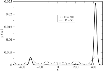
Figure 1: Density estimation for the variable $x_{1}$ of the Schwefel function. Two different diffusion constants have been considered, taking $L=100$ in both cases. In the two cases the density clearly represents the structure of the cost function. The density is sharply peaked around the optimal value for the lesser $D$.

In contrast to the Schwefel function, the stochastic search process associated to the Levy No. 5 problem represents a coupled nonlinear dynamics. Despite that this problem has about $760$ local minima [18], the estimation algorithm shows good convergence properties, as is illustrated in Fig. 2.

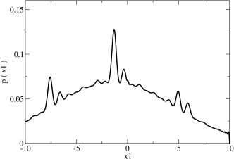
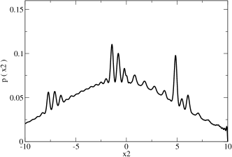
Figure 2: Probability densities associated to the Levy No. 5 problem, using the parameter values $L=200$, $D=70$ and $M=300$. The densities maxima are at coordinates $(-1.3,-1.42)$.

The two previous examples show how, once that the estimation algorithm as attained convergence, is possible to define a region of the search space in which with high probability the global optimum is located. This concept is more sistematically studied through the introduction of normalized distances. The distance normalized with respect to the search space $L_{1,n}\leq x_{n}\leq L_{2,n}$ between two points $x$ and $x^{*}$ is defined by

$$distance=\sqrt{\frac{(x_{1}-x^{*}_{1})^{2}+...+(x_{N}-x^{*}_{N})^{2}}{(L_{1,1}-L_{2,1})^{2}+...+(L_{1,N}-L_{2,N})^{2}}}.$$ (11)

Two measures written in terms of normalized distances are presented in the examples of Figures 3, 4 and 5: i) The distance between the global optimum and the point in which the density is maximum. ii) The length of the $95\%$ probability interval around the point of maximum probability.

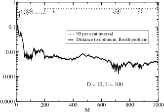
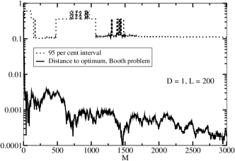
Figure 3: Density estimation for the Booth problem. Semi – log scale has been used.

Figure 4: Density estimation for the Colville problem.

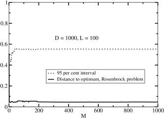
Figure 5: Density estimation for the Rosenbrock problem.

Under general conditions a Gibbs sampling displays geometric convergence [19]. In the presented experiments the running time has been chosed such that the $95\%$ probability interval differ in less than $0.01$ between succesive iterations. Additionally, several control runs from different and independent starting conditions have been performed, indicating convergence to the same corresponding region within the predefined accuracy. As expected for a Gibbs sampling, the density appears to contract to a region of space that is independent of the staring point [20]. The numerical realizations suggest that convergence is attained at a few hundreds of iterations for all of the examples, even for the $20$ – dimensional Rosenbrock problem, which as been reported to be difficult to solve by stochastic heuristics like genetic algorithms [21].

The numerical experiments show that the global optimum is contained in a region close to the point of maximum probability, and that this region gets more sharp as $D$ decreases. A straighforward application of this behavior would be, for instance, on simulated annealing – type algorithms. Starting with a large diffusion constant, search regions can be iteratively discarded. By the use of the density estimation method, a probability measure is associated with each region. In this way the user can define a certain level of precision in the search. Several statistical quantities can be readily calculated like measures of confidence, for instance probability intervals or characteristic fluctuation sizes.

Because the estimation algorithm depends on linear operations only, additional nonlinearities in the cost function can be treated with essentialy the same efficiency, giving more freedom and flexibility in modeling. For instance, the application of the density estimation algorithm to constrained problems can be done in a very direct manner through the addition of suitable “energy barriers” (or more precisely, “force barriers”). These barriers don’t need to be very large. Their main purpose is not to define prohibited regions, but only regions with low probability. The original constrained problem is transformed to an unconstrained cost function with additional nonlinearities. Of course, the design of adequate barriers may be a difficult problem – dependent task. However, at least for some problems the approach seems to be straightforward. This is illustrated on the classical NP-hard knapsack problem [22]. It is well known that many standard instances of the knapsack model can be efficiently solved by exact methods [22], which makes it an ideal example for experimentation with the density estimation algorithm. The knapsack problem is formulated as

$$min\quad-\sum_{n=1}^{N}q_{n}x_{n}$$ (12)

$$s.t.\quad\sum_{n=1}^{N}w_{n}x_{n}\leq c,$$

$$-x^{2}_{n}+x_{n}\leq 0,\quad 0\leq x_{n}\leq 1,$$

where $q_{n}$, $w_{n}$ and $c$ are positive numbers. The quadratic constraint is equivalent to the usual restriction to binary variables. The following transformation is proposed,

$$min\quad-\sum_{n=1}^{N}q_{n}x_{n}$$ (13)

$$+k_{0}\sum_{n=1}^{N}\frac{1}{1+exp(-b_{0}[-x^{2}_{n}+x_{n}])}$$

$$+k_{1}\frac{exp\left(b_{1}[\sum_{n=1}^{N}w_{n}x_{n}-c]\right)-1}{exp\left(-b_{2}[\sum_{n=1}^{N}w_{n}x_{n}-c]\right)+1}$$

$$s.t.\quad 0\leq x_{n}\leq 1,$$

For illustrative purposes, consider the instance $q=(2,3,5)$, $w=(3,5,7)$, $c=10$ of the knapsack problem. By inspection, the solution is given by $x=(1,0,1)$. In Fig. 6 typical densities produced by the estimation algorithm for this instance are shown. The selection of the parameters has been done after the performance of short runs, measuring the effects of each of the nonlinear terms. The parameters have been tuned such that: a) The first nonlinear term alone produce symmetric densities peaked in the neighborhood of $\{0,1\}$. b) The addition of the second nonlinear term and the original cost function generate densities in which the configurations with maximum probabilty satisfy the $\sum_{n=1}^{N}w_{n}x_{n}\leq c$ constraint. Notice that the configuration that corresponds to the global optimum has the maximum probability.

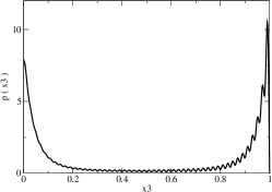
Figure 6: Probability densities associated to a three dimensional instance of a knapsack problem.

A larger example is presented in Fig. 7. The exact solution has been calculated with the branch and bound algorithm supplied in the GNU Linear Programming Kit [23]. The instance has been generated by taking $w_{n}$ uniformily distributed in an interval $[1,R]$, and

$$q_{n}=w_{n}+(\varepsilon_{n}-1)\frac{R}{100}+\frac{R}{10},$$ (14)

$$\varepsilon_{n}\quad uniform\quad deviate\quad in\quad[-1,1],$$

which imply strong linear correlations between $q_{n}$ and $w_{n}$. Instances of this kind are relevant to real management problems in which the return of an investment is proportional to the sum invested within small variations [22]. It has been argued that these type of instances fall in a category which is close to the “worst case” scenario for exact algorithms [22]. Despite of that, the estimation method converge to densities in which the optimum is contained in a region with high probability. Moreover, from the definition of the normalized distance, follows that the closest integers to the elements of the vector that represent the point of maximum probability differ in $\sim 1$ positions from the exact solution.

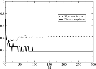
Figure 7: The density estimation of an instance of a knapsack problem with $30$ variables.

Three independent realizations of the numerical experiment over instances generated by Eq. (14) have been performed, varying the orders of magnitude of $R$ and $c$. The results are summarized in Table 1, indicating the number of $0\leftrightarrow 1$ flips that the normalized distances imply.

Table 1: Density estimation on instances of the knapsack problem with $30$ variables. The final two columns indicate the resulting $95\%$ intervals and gaps to optimum like normalized distances/flips.

$R$	$c$	$k_{0}$	$k_{1}$	$b_{0}$	$b_{1}$	$b_{2}$	$M$	$L$	$D$	Interval  Gap
$10$	$100$	$10$	$7.1$	$10$	$0.01$	$2b_{1}$	$300$	$100$	$1$	$0.425$/$5$  $0.185$/$1$
$100$	$500$	$100$	$37.0$	$10$	$0.001$	$3b_{1}$	$300$	$100$	$15$	$0.432$/$6$  $0.363$/$4$
$1000$	$3000$	$1000$	$315.0$	$10$	$0.0001$	$3b_{1}$	$300$	$100$	$100$	$0.433$/$6$  $0.257$/$2$

It should be remarked that, although the instances of the knapsack model discussed in this section are quickly solvable by exact algorithms, no reference to the particular structure of the original problem has been used for the density estimation. In fact, the problem has been treated like a highly nonlinear cost function of $30$ variables.

3 Heuristics Based on Stationary Density Estimation

The potential benefits of the stationary density estimation algorithm as a tool for the construction of new heuristics for high dimensional global optimization problems is illustrated through the following greedy random search procedure:

1) Run an iteration of the stationary density estimation algorithm.

2) An initial best point is given by the global maximum of the estimated density

3) Define a population of $N+1$ points. One point is the current best solution and other is the current point with maximum probability density. The remaining $N-1$ points are randomly drawn from an uniform distribution centered around the best point. For each dimension, the corresponding uniform distribution has a length equal to the typical fluctuation size given by the estimated density.

4) Run a downhill simplex routine. The starting conditions are given by the simplex defined by the points generated at step 3 as vertices.

5) If from step 4 results a point which improves the best known objective value, then update the best point.

6) Run an iteration of the density estimation algorithm.

7) Go to step 3.

From an evolutionary perspective, the above procedure acts at two different levels. At a short time scale finite populations evolve locally in a very greedy fashion. On the other hand, large changes on the population composition are dictated by a long time scale dynamics, which is consistent with the learned information about the global cost landscape. This information is gained through the approximation of the long term statistical density of a diffusive search process.

The short time scale exploration of the solution space is dominated by the downhill simplex method, which is a deterministic search based on function evaluations of a simplex vertices [24]. In a $N$ dimensional search space, a population of $N+1$ points defined by the corresponding $N+1$ vertices evolve under simple geometric transformations, namely reflection, expansion and contraction. At each iteration, a new trial point is generated by the image of the worst point in the simplex (reflection). If the new point is better than all other vertices, the simplex expands in its direction. If the trial point improves the worst point, a reflection from the new worst point is performed. A contraction step is made when the worst point is at least as good as the reflected point. In this way the simplex eventually surrounds a local minimum. In the experiments presented here, the implementation of the downhill simplex given by [17] has been used, with a fractional decrease of cost value of at least $10e-4$ as termination criteria. A maximum of $50000$ function evaluations in the downhill simplex routine is allowed.

From a given reference point $x^{(best)}$, an initial simplex for each call to the downhill simplex routine is defined through the characteristic length scales $\lambda_{n}$, as $x^{(i)}=x^{(best)}+\lambda_{n}e_{n}$ where the $e_{n}$ are $N$ unit vectors. The estimated long term density provides a vertex (the point with maximum likelihhood at the current stage) and most importantly, typical fluctuation sizes, denoted by $\sigma_{n}$. These are given by the first two moments of the estimated density,

$$\sigma_{n}=\sqrt{\left<x_{n}^{2}\right>-\left<x_{n}\right>^{2}}$$ (15)

Due to the simple form of the expansion of the estimated density, all the integrals over the variables domain that are needed for moment calculation are performed analitically. The resulting expressions are finite sums with $L$ terms.

The typical fluctuation sizes (15) provide a natural definition for the characteristic length scales $\lambda_{n}$, in the sense expressed in step (3) of the greedy diffusive search described above.

For illustration purposes, consider the Rosenbrock test function. In Fig.8 are presented some plots of the beahavior of our greedy stochastic search for the Rosenbrock problem of $N=20$ variables. The graphs represent the cost function values over successive iterations. Four samples from a total of $100$ runs are plotted. The result of a version of the algorithm in which an uniform density over the search space is used instead of the estimated long term density is also plotted. The success in finding the optimum is defined by a gap size with the known global optimum lesser than $0.001$. Each run consist of $100$ iterations. Over the total number of runs of the greedy stochastic search, $90\%$ have been successful, and the $100\%$ of the runs outperform the search based on uniform distributions. An $80\%$ of the runs have been successful in less than $48$ iterations and $30\%$ in less than $13$ iterations. For the $13$ iterations cases, an average number of $28080$ cost function evaluations was needed. It should be remarked that the $20$-dimensional Rosenbrock test function has been reported to be extremely difficult to solve by randomized optimization algorithms. For instance, in an experiment similar to the one presented here, it has been reported in [25] a success rate of zero after $400000$ function evaluations for Simulated Annealing, Cross–Entropy and Model Reference Adaptive Search. On the other hand, in [21] is reported that Genetic Algorithms and Scatter Search methods are unable to succeed in the $20$-dimensional Rosenbrock problem after $50000$ cost function evaluations.

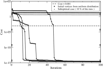
Figure 8: Greedy stochastic search for the Rosenbrock problem. The parameter values of the density estimation are $L=30$ and $D=10000$.

A more exhaustive experimentation with possible heuristics based on the stationary density estimation algorithm is in progress.

4 Conclusion

The presented results strongly suggest that the proposed density estimation algorithm can be used to construct probabilistic bounds on the location of global optima for large classes of problems. The density estimation is performed in a well defined number of elementary operations. The developed theory and the numerical experiments indicate that any given desired precision on the bounds can be attained with some finite values of the basic parameters, performing a finite number of iterations. The total computational cost per iteration grows linearly with problem size. The algorithm estimates the marginal density of each separate variable, which makes it suitable for parallel implementation. These features make the proposed method a promising tool, opening the possibility of constructing probabilistic optimal certificates for large scale unstructured problems. Experimentation in this direction is in progress. On the other hand, the density estimation algorithm may be used to develop new heuristics or improve existing stochastic or deterministic algorithms.

References

References

- [1] Kirkpatrick, S, Gelatt Jr., C D and Vecchi M P Optimization by Simulated Annealing, 1983 Science 220 671-680.
- [2] Gidas, B in Topics in Contemporary Probability and its Applications, 1995 (Prob. Stochastic Ser., CRC) pp. 159-232.
- [3] Parpas, P, Rustem, B and Pistikopoulos, E N Linearly Constrained Global Optimization and Stochastic Differential Equations 2006 Journal of Global Optimization, 36, 2 191-217.
- [4] Geman, S and Hwang, C R Diffusions for Global Optimization 1986 SIAM J. Control Optim. 24, 5 1031-1043.
- [5] Goldberg D Genetic Algorithms in Search, Optimization and Machine Learning, 1989 (Addison- Wesley).
- [6] Eiben, A E and Smith, J E Introduction to Evolutionary Computing, 2003 (Springer).
- [7] Pelikan M, Goldberg D E and Lobo F G A Survey of Optimization by Building and Using Probabilistic Models, 2002 Computational Optimization and Applications 21 1 5-20.
- [8] Floudas C A Deterministic Global Optimization: Theory, Methods and Applications, 2000 (Kluwer).
- [9] Horst, R, Pardalos P M and Thoai N V Introduction to Global Optimization, 1995 (Kluwer) pp. 158-183.
- [10] Metropolis, N, Rosenbluth A, Rosenbluth M, Teller A and Teller E Equations of State Calculations by Fast Computing Machines, 1953 Journal of Chemical Physics 21 1087-1092.
- [11] Suykens, J A K, Verrelst, H and Vandewalle, J On–Line Learning Fokker–Planck Machine 1998 Neural Processing Letters, 7, 2 81-89.
- [12] Risken, H The Fokker–Planck Equation, 1984 (Springer).
- [13] Van Kampen, N G Stochastic Processes in Physics and Chemistry, 1992 (North-Holland).
- [14] Grasman, J and van Herwaarden, O A Asymptotic Methods for the Fokker–Planck Equation and the Exit Problem in Applications, 1999 (Springer).
- [15] Geman S and Geman D Stochastic relaxation, Gibbs distributions, and the Bayesian restoration of images, 1984 IEEE Trans. Pattern Anal. Machine Intell. 6 721-741.
- [16] Berrones, A in Proceedings of the 9th International Work-Conference on Artificial Neural Networks 2007 (IWANN 2007), Lecture Notes in Computer Science 4507 (Springer) pp. 1-8.
- [17] Press, W, Teukolsky, S, Vetterling, W and Flannery, B Numerical Recipes in C++, the Art of Scientific Computing, 2005 (Cambridge University).
- [18] Parsopoulos, K E and Vrahatis, M N Recent approaches to global optimization problems through Particle Swarm Optimization, 2002 Natural Computing 1 235-306.
- [19] Roberts, G O and Polson N G On the Geometric Convergence of the Gibbs Sampler 1994 J. R. Statist. Soc. B 56 2 377-384.
- [20] Canty, A Hypothesis Tests of Convergence in Markov Chain Monte Carlo 1999 Journal of Computational and Graphical Statistics 8 93-108.
- [21] Laguna, M and Martí, R Experimental Testing of Advanced Scatter Search Designs for Global Optimization of Multimodal Functions. Journal of Global Optimization, 2005 Journal of Global Optimization 33 2 235-255.
- [22] Pisinger, D Where are the hard knapsack problems? 2005 Computers and Operations Research 32 9 2271-2284.
- [23] http://www.gnu.org/software/glpk/
- [24] Nelder J A and Mead R A simplex method for function minimization, 1965 Computer Journal, 7, 308-313.
- [25] Hu J, Fu M and Marcus, S A Model Reference Adaptive Search Method for Global Optimization, 2007 Operations Research, 55, 3, 549–568.