HE 0515–4414 – an unusual sub-damped Ly $\alpha$ system revisited ^,

Abstract

Aims. We examine the ionization, abundances, and differential dust depletion of metals, the kinematic structure, and the physical conditions in the molecular hydrogen-bearing sub-damped Ly $\alpha$ system toward HE 0515-4414.

Methods. We used the STIS and VLT UVES spectrographs to obtain high-resolution recordings of the damped Ly $\alpha$ profile and numerous associated metal lines. Observed element abundances are corrected with respect to dust depletion effects.

Results. The sub-damped Ly $\alpha$ absorber at redshift $z=1.15$ is unusual in several aspects. The velocity interval of associated metal lines extends for $700$ km s^-1. In addition, saturated H i absorption is detected in the blue damping wing of the $N_{\mathrm{{H\textsc{i}}}}=8\times 10^{19}$ cm^-2 main component. The column density ratios of associated Al ii, Al iii, and Fe ii lines indicate that the absorbing material is ionized. 19 of in total 31 detected metal line components are formed within peripheral H ii regions, while only 12 components are associated with the predominantly neutral main absorber. The bimodal velocity distribution of metal line components suggests two interacting absorbers. For the main absorber the observed abundance ratios of refractory elements to Zn range from Galactic warm disk $[\mathrm{Si}/\mathrm{Zn}]_{\mathrm{g}}=-0.40\pm 0.06$, $[\mathrm{Fe}/\mathrm{Zn}]_{\mathrm{g}}=-1.10\pm 0.05$ to halo-like and essentially undepleted patterns. The dust-corrected metal abundances indicate a nucleosynthetic odd-even effect and might imply an anomalous depletion of Si relative to Fe for two components, but otherwise do correspond to solar ratios. The intrinsic average metallicity is almost solar $[\mathrm{Fe}/\mathrm{H}]_{\mathrm{m}}=-0.08\pm 0.19$, whereas the uncorrected average is $[\mathrm{Zn}/\mathrm{H}]_{\mathrm{g}}=-0.38\pm 0.04$. The ion abundances in the periphery conform with solar element composition.

Conclusions. The detection of H ii as well as the large variation in dust depletion for this sight line raises the question whether in future studies of damped Ly $\alpha$ systems ionization and depletion effects have to be considered in further detail. Ionization effects, for instance, may pretend an enrichment of $\alpha$ elements. An empirical recipe for detecting H ii regions is provided.

1 Introduction

The study of QSO absorption lines provides vital information on the nucleosynthetic history of the universe by complementing the compositional analysis of stars and interstellar space in local galaxies with element abundances at higher redshift. In particular, interests are focused on extragalactic structures termed damped Ly $\alpha$ (DLA) systems, essentially comprised of neutral hydrogen with column densities $N_{H\textsc{i}}\geq 2\times 10^{20}$ atoms cm^-2 (for a review see Wolfe et al., 2005). Absorbers in the sub-DLA range with column densities $N_{H\textsc{i}}\geq 10^{19}$ atoms cm^-2 might be mainly neutral when the ionizing background is reduced (Péroux et al., 2002, 2003). The aim of these examinations is to establish accurate element abundances for the aggregations of neutral gas that are examples of interstellar environments in the high-redshift universe. Since the measurement of metal column densities is straightforward, the only problem is their correct interpretation.

The true nature of DLA systems is unknown and the underlying population, being constituted of hierarchical structures with different morphologies, chemical enrichment histories, and physical environments, is multifarious. The diversity is attested by the disparate values obtained for metal abundances at any given redshift.

The metallicity of DLA systems is not correlated with their column density, however, there is an upper bound for distribution of column densities versus metallicity (Boissé et al., 1998). Though there are high column density DLA absorbers with high metallicity in the foreground of the star forming hosts of gamma-ray bursts (Watson et al., 2005), similar absorbers are not detected toward QSOs. The cosmic mean metallicity of DLA absorbers increases with cosmic time (Prochaska et al., 2003; Kulkarni et al., 2005; Rao et al., 2005), but is an order of magnitude lower than predicted by cosmic star formation history (see the discussion of the missing metals problem by Wolfe et al., 2005). The solution to this problem is a matter of debate. Conclusive evidence of enriched material ejected from DLA absorbers into the intergalactic medium or of active star formation restricted to compact regions is missing. The latter possibility is closely linked to the physical properties of the interstellar medium and its molecular content (Wolfe et al., 2003b, a). Molecular gas is uncommon in DLA absorbers. If found, the fraction of molecular hydrogen, usually between $10^{-6}$ and $10^{-2}$, is not correlated with the column density of atomic hydrogen (Ledoux et al., 2003). However, Petijean et al. (2006) have demonstrated that the presence of molecular hydrogen at high redshift is strongly correlated with the metallicity.

Since the spectroscopic analysis is restricted to the gaseous phase of the absorbing medium, observed element abundances are potentially distorted by dust removing atoms in varying amounts, depending on their affinity to the solid state. In particular high-metallicity and molecule-bearing absorbers are affected by dust (Petijean et al., 2002; Ledoux et al., 2003). Depletions are largely lower than in the Galactic halo, but increase with metallicity (Vladilo, 2004). In practice, the observed element abundances are corrected ad hoc, using Galactic interstellar depletion patterns as reference (Vladilo, 2002b, a). Another aspect of dust is the possibility that DLA absorbers may elude detection because the background QSOs are obscured (Fall & Pei, 1993). The selection effects are complicated since obscurement is counteracted, but not compensated, by amplification due to gravitational lensing (Smette et al., 1997). The effect of dust is subject of several studies (Murphy & Liske, 2004; Quast et al., 2004b; Akerman et al., 2005; Smette et al., 2005; Vladilo & Péroux, 2005; Wild et al., 2005). A further difficulty are ionization effects. Examples of DLA-associated metal line components formed within mainly ionized material are given by Prochaska et al. (2002) and Dessauges-Zavadsky et al. (2006).

The column density distribution and kinematic structure of absorbers provide important constraints on hierarchical structuring (e.g. Cen et al., 2003; Nagamine et al., 2004) and immediate insight into the processes of galaxy formation (Wolfe & Prochaska, 2000). The extended multicomponent velocity structure and characteristic asymmetry of DLA-associated metal lines is consistent with galaxy formation models in hierarchic cold dark matter cosmologies, and reproducible by the hydrodynamical simulation of rotation, random motion, infall, and merging of irregular protogalactic clumps hosted by collapsed dark matter halos (Haehnelt et al., 1998). The velocity structure of sub-DLA absorbers compares to that of the higher column density systems (Péroux et al., 2003), which is unexpected since semianalytic galaxy formation models (Maller et al., 2001, 2003) predict markedly different kinematic properties. The absorption velocity intervals of both sub-DLA and DLA absorbers typically extend for $100$ km s^-1. More extended systems tend to higher metallicities and lower hydrogen column densities (Wolfe & Prochaska, 1998). In particular the latter property is unexpected and difficult to interpret in terms of rotating disks models. The most extended systems, however, are probably due to interacting or merging galaxies (Petijean et al., 2002; Richter et al., 2005). Strong observational evidence for a correlation between DLA metallicity and absorption profile velocity spread, which probably is the consequence of a mass-metalicity relation, has recently been provided by Ledoux et al. (2006).

In this study we revisit the $z=1.15$ sub-DLA system toward HE 0515–4414 (Reimers et al., 1998; de la Varga et al., 2000). The main components of associated metal lines exhibit excited neutral carbon and molecular hydrogen (Quast et al., 2002; Reimers et al., 2003). Most outstanding, the absorption velocity interval extends for $700$ km s^-1. Based on refined spectroscopy, we examine the ionization, abundances, and differential dust depletion of metals as well as the kinematic structure, and physical conditions of this unusual absorption line system.

2 Observations

Ranging from the NUV to the end of the visual, the observations cover the sub-damped profile at 2615 Å (Fig. 1) and numerous associated metal lines (Fig. 2).

Table 1: Details of spectra obtained with UVES

Date	Obs.	Exp. (s)	Mode	Arm	Wav. (Å)
2000-10-07	101818	4500	DI2	blue	3460
		4499		red	8600
2000-11-16	101822	4500	DI1	blue	3460
		4499		red	5800
2000-11-17	101821	4500	DI1	blue	3460
		4499		red	5800
2000-11-18	101820	4500	DI1	blue	3460
		4499		red	5800
2000-12-15	101812	3600	DI2	blue	4370
		3599		red	8600
	101813	3600	DI2	blue	4370
		3600		red	8600
	101814	3600	DI2	blue	4370
		3599		red	8600
2000-12-16	101811	3600	DI2	blue	4370
		3600		red	8600
2000-12-21	101810	3600	DI2	blue	4370
		3599		red	8600
	101815	3600	DI2	blue	4370
		3599		red	8600
2000-12-23	101817	4500	DI2	blue	3460
		4500		red	8600
2000-12-24	101819	4500	DI1	blue	3460
		4500		red	5800
2001-01-02	101816	4500	DI2	blue	3460
		4500		red	8600

2.1 UV-visual spectroscopy

HE 0515–4414 was observed during ten nights between October 7, 2000 and January 3, 2001, using the UV-Visual Echelle Spectrograph (UVES) installed at the second VLT Unit Telescope (Kueyen). Thirteen exposures were made in the dichroic mode using standard settings for the central wavelengths of 3460/4370 Å in the blue, and 5800/8600 Å in the red (Table 1). The CCDs were read out in fast mode without binning. Individual exposure times were 3600 and 4500 s, under photometric to clear sky and seeing conditions ranging from 0.47 to 0.70 arcsec. The slit width was 0.8 arcsec providing a spectral resolution of about 55 000 in the blue and slightly less in the red. The raw data frames were reduced at the ESO Quality Control Garching using the UVES pipeline Data Reduction Software. Finally, the individual vacuum-barycentric corrected spectra were combined resulting in an effective signal-to-noise ratio per pixel of 90-140.

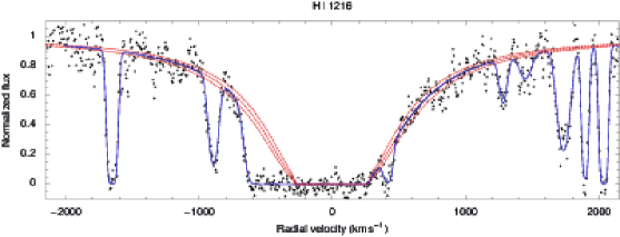
Figure 1: STIS Echelle order showing the sub-damped H i profile with redshift $z=1.15$. The solid curve indicates the optimized profile decomposition of the spectrum, while the dashed curves mark the damped profile. The blue damping wing is blended with further H i absorption which is associated with numerous metal lines (Fig. 2). The origin of the radial velocity axis corresponds to the redshift $z=1.15080$

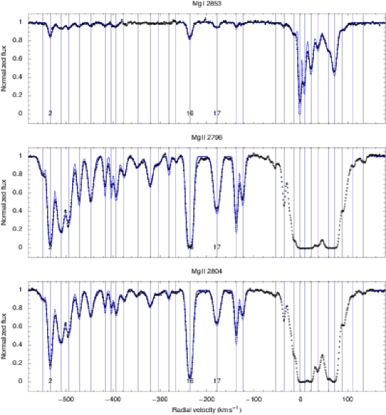
Figure 2: Metal lines associated with the sub-damped profile shown in Fig. 1. The dashed and solid curves indicate the optimized profile decomposition and its instrumental convolution. Individual components are marked by vertical lines. Data represented by empty circles are ignored in the profile decomposition. Components 3, 16, and 17 possibly are unresolved blends (Quast et al., 2004a). This figure is continued in the Online Material

2.2 NUV spectroscopy

The UV-visual recordings were supplemented by spectra obtained with the Space Telescope Imaging Spectrograph (STIS) during three orbits between January 31 and February 1, 2000, ranging from 2300 to 3100 Å. The total exposure time was 31 500 s, while the instrument was operating in the medium resolution NUV mode (E230M) with the entrance aperture of $0\aas@@fstack{\prime\prime}2\times 0\aas@@fstack{\prime\prime}2$ providing a spectral resolution of about 30 000. The raw spectra were reduced at the Space Telescope Science Institute using the STIS pipeline software completed by an additional interorder background correction. The combined spectra show an effective signal-to-noise ratio per pixel of 5-10.

3 Line profile analysis

There are several basically different techniques for the analysis of QSO absorption lines: the classical line profile decomposition, the apparent optical depth method (Savage & Sembach, 1991), and Monte Carlo inversion (Levshakov et al., 2000). While the classical profile decomposition postulates discrete homogenous absorbers with Gaussian (i.e. thermal or microturbulent) particle velocity distributions, the apparent optical depth technique allows the very direct interpretation of observed spectra without the need to consider the velocity structure of spectral lines as long as the absorption is optically thin or sufficiently resolved. Otherwise, the apparent optical depth is not representative and additional operations are required to recover the correct column density (Jenkins, 1996). The corrective procedure, however, is only approved for synthetic spectra with Gaussian velocity distributions underlying the individual components. Monte Carlo inversion considers random velocity and density fields along the sight line, but requires photoionization calculations to connect the random fields to the observed absorption that are too time-consuming for DLA systems.

Since we consider many blended or optically thick lines, we prefer the classical decomposition technique for the analysis and use the apparent optical depth method to supplement the diagnostics. Throughout the analysis we use the atomic data compiled by Morton (2003).

3.1 Line profile decomposition

The general problem of line profile decomposition in QSO spectra and its solution by means of evolutionary forward modelling is described in detail by Quast et al. (2005). For the specific purpose of measuring accurate metal column densities we introduce several additional constraints:

1. Each metal line component is modelled by a superposition of Doppler profiles positioned at the same radial velocity. This procedure helps to recover the velocity structure of the instrumentally blurred line ensembles and ensures the calculation of elemental abundances for concentric velocity intervals.

2. For any component all lines corresponding to the same atomic or ionic species are modelled by Doppler profiles of the same broadening velocity and column density. With respect to their broadening velocities all Cr ii, Mn ii, Fe ii, Ni ii, and Zn ii lines are modelled as if corresponding to the same ionic species. The same treatment is applied to Al ii and Al iii lines.

3. Asymmetric lines like unresolved blends are modelled by a single component if the individual components of the blend are separated by less than the full width at half maximum of the instrumental profile.

4. Single absorption features with column density $\log N<13.8-\log\lambda f$ are ignored.

All metal line ensembles are decomposed simultaneously while the local background continuum is approximated by an optimized linear combination of Legendre polynomials extending to the nearest absorption-free regions. The metal line recordings of STIS are too noisy and too contaminated with Lyman forest lines to be considered in the decomposition. The STIS Echelle order showing the sub-damped profile is decomposed using pseudo-Voigt profiles (Ida et al., 2000). The profile is well defined by its Lorentzian part and can be distinguished from even a curved background continuum due to its symmetry. Note that the blue damping wing is blended with further H i absorption which, however, does provide only little information since due to saturation the solution is ambiguous. For convenience, the blended absorption is modelled by two components of the same width, and central wavelengths in accord with the strongest associated metal lines (Fig. 1).

3.2 Apparent optical depth analysis

The apparent optical depth method is only applied to the weaker transitions of a given atomic or ionic species to avoid narrow saturation. The spectra are normalized using the optimized continuum approximation obtained from the line profile decomposition. The normalized flux is averaged using a moving window of 10 km s^-1. Low apparent optical depths $\tau_{\mathrm{a}}\leq 0.01$ are clipped.

4 Results and discussion

In this section we present the optimized profile decomposition and examine the ionization, chemical composition and dust content, kinematic structure, and physical conditions in the absorbing medium.

4.1 Profile decomposition

The optimized decomposition of the sub-damped Ly $\alpha$ profile and associated metal lines is depicted in Figs. 1-4. The corresponding line parameters are listed in Tables 2 and 3. Since only the metal line components 20-31 are associated with the sub-damped profile, components 1-19 and 20-31 are termed peripheral and main components, respectively. Note that components 23 and 24 correspond to the neutral carbon and H₂-bearing components considered by Quast et al. (2002) and Reimers et al. (2003).

Table 2: Optimized decomposition of the sub-damped profile shown in Fig. 1. The listed numbers correspond to a straight continuum, for a curved continuum the errors increase. The origin of the radial velocity (RV) scale corresponds to the redshift $z=1.15080$. Note that the non-damped absorption does provide only little information. The line parameters are listed for completeness only

Transition	$\phantom{-}\mathrm{RV}$ (km s-1)	$b$ (km s-1)	$\log N$ (cm-2)
H i 1216	$-3.19\pm 11.14$	$75.17\pm 5.84$	$19.89\pm 0.03$
H i 1216	$-236.14$	$82.74\pm 7.23$	$16.84\pm 0.92$
H i 1216	$-533.51$	$82.74\pm 7.23$	$14.98\pm 0.13$

Table 3: Optimized decomposition of the metal lines shown in Figs. 2 and 3. This list is abridged for convenience, the complete table is available in the Online Material

No.	Transitions		$\phantom{-}\mathrm{RV}$ (km s-1)	$b$ (km s-1)	$\log N$ (cm-2)
23	Mg i	2026, 2853	$-1.61\pm 0.03$	$2.16\pm 0.05$	$12.41\pm 0.03$
23	Al ii	1671	$-1.61$	$3.05$	$13.86\pm 0.17$
23	Al iii	1855, 1863	$-1.61$	$3.05$	$11.50\pm 0.06$
23	Si i	2515	$-1.61\pm 0.03$	$2.17\pm 2.10$	$11.34\pm 0.08$
23	Si ii	1527, 1808	$-1.61\pm 0.03$	$3.05\pm 0.09$	$14.28\pm 0.03$
23	S i	1807	$-1.61\pm 0.03$	$1.56\pm 1.12$	$12.18\pm 0.05$
23	Ca ii	3935	$-1.61\pm 0.03$	$2.15\pm 0.10$	$12.12\pm 0.02$
23	Cr ii	2056, 2062	$-1.61\pm 0.03$	$2.97\pm 0.05$	$11.84\pm 0.06$
23	Mn ii	2577, 2594, 2606	$-1.61\pm 0.03$	$2.97\pm 0.05$	$11.51\pm 0.03$
23	Fe i	2484, 2524	$-1.61\pm 0.03$	$0.48\pm 0.18$	$11.30\pm 0.06$
23	Fe ii	1608, 2344, 2374, 2383, 2587, 2600	$-1.61\pm 0.03$	$2.97\pm 0.05$	$13.51\pm 0.01$
23	Ni ii	1710, 1742, 1752	$-1.61\pm 0.03$	$2.97\pm 0.05$	$12.48\pm 0.04$
23	Zn ii	2026, 2063	$-1.61\pm 0.03$	$2.97\pm 0.05$	$11.79\pm 0.02$
24	Mg i	2026, 2853	$\phantom{-}7.63\pm 0.06$	$4.09\pm 0.12$	$11.90\pm 0.01$
24	Al ii	1671	$\phantom{-}7.63$	$5.36$	$12.82\pm 0.04$
24	Al iii	1855, 1863	$\phantom{-}7.63$	$5.36$	$11.72\pm 0.05$
24	Si ii	1527, 1808	$\phantom{-}7.63\pm 0.06$	$5.36\pm 0.25$	$14.16\pm 0.04$
24	Ca ii	3935	$\phantom{-}7.63\pm 0.06$	$3.17\pm 0.17$	$11.78\pm 0.01$
24	Cr ii	2056, 2062	$\phantom{-}7.63\pm 0.06$	$4.92\pm 0.13$	$11.61\pm 0.14$
24	Mn ii	2577, 2594, 2606	$\phantom{-}7.63\pm 0.06$	$4.92\pm 0.13$	$11.36\pm 0.03$
24	Fe ii	1608, 2344, 2374, 2383, 2587, 2600	$\phantom{-}7.63\pm 0.06$	$4.92\pm 0.13$	$13.36\pm 0.01$
24	Ni ii	1710, 1742, 1752	$\phantom{-}7.63\pm 0.06$	$4.92\pm 0.13$	$12.33\pm 0.06$
24	Zn ii	2026, 2063	$\phantom{-}7.63\pm 0.06$	$4.92\pm 0.13$	$11.59\pm 0.03$
28	Mg i	2026, 2853	$\phantom{-}72.54\pm 0.06$	$6.03\pm 0.15$	$11.77\pm 0.01$
28	Al ii	1671	$\phantom{-}72.54$	$6.14\pm 0.15$	$12.57\pm 0.02$
28	Al iii	1855, 1863	$\phantom{-}72.54$	$6.14\pm 0.15$	$11.17\pm 0.13$
28	Si ii	1527, 1808	$\phantom{-}72.54\pm 0.06$	$6.45\pm 0.18$	$13.75\pm 0.02$
28	Ca ii	3935	$\phantom{-}72.54\pm 0.06$	$5.52\pm 0.13$	$12.08\pm 0.01$
28	Cr ii	2056, 2062	$\phantom{-}72.54\pm 0.06$	$5.81\pm 0.09$	$11.92\pm 0.06$
28	Mn ii	2577, 2594, 2606	$\phantom{-}72.54\pm 0.06$	$5.81\pm 0.09$	$11.34\pm 0.03$
28	Fe ii	1608, 2344, 2374, 2383, 2587, 2600	$\phantom{-}72.54\pm 0.06$	$5.81\pm 0.09$	$13.51\pm 0.01$
28	Ni ii	1710, 1742, 1752	$\phantom{-}72.54\pm 0.06$	$5.81\pm 0.09$	$12.32\pm 0.06$
28	Zn ii	2026, 2063	$\phantom{-}72.54\pm 0.06$	$5.81\pm 0.09$	$10.72\pm 0.11$

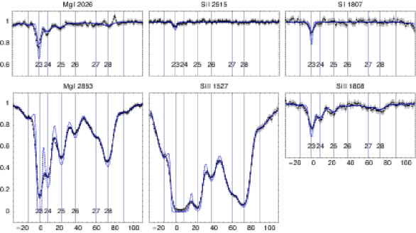
Figure 3: Close-up of associated metal lines. Individual components are labeled by numbers 23-28

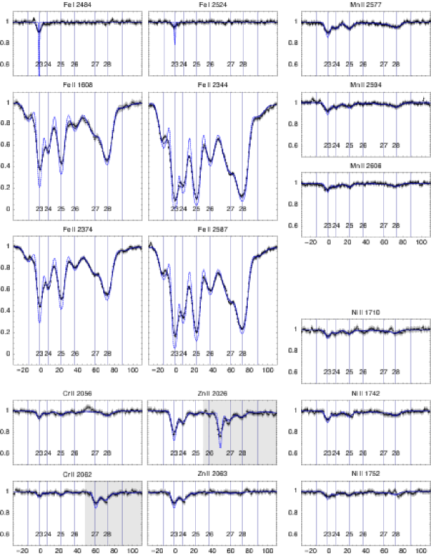
Figure 3: continued. The shadings mark the main components of the Mg i $\lambda 2026$ and Zn ii $\lambda 2063$ lines. Note that the detection of Fe i and Si i has been reported earlier by Quast et al. (2004b)

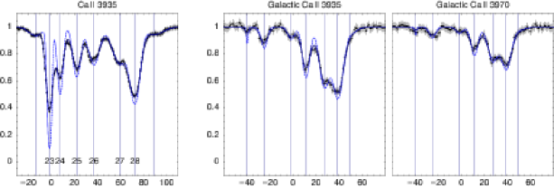
Figure 4: Associated Ca ii lines (left panel) compared with interstellar Ca ii absorption in the Galactic halo along the same line-of-sight

4.1.1 Peripheral components 1-19

The decomposition of the peripheral components is defined by the structure of Mg i, Mg ii, Si ii, and Fe ii lines. Part of the Si ii profile is ignored due to contamination by Lyman forest lines. The weakest components with $10^{11}$ metal ions cm^-2 are indicated by the Mg ii lines, whereas the components exceeding $10^{13}$ ions cm^-2 are saturated for Mg ii, but well defined for Fe ii. Nonetheless, the decomposition is uncertain in detail, since components 3, 16, and 17 possibly are unresolved blends. The ambiguities, however, do not affect the chemical abundance analysis.

For some components the Fe ii lines are narrower than those corresponding to lighter elements. The constraints on the decomposition of Fe ii, however, are much stronger than those on the rest of lines. The evidence of thermal broadening is therefore not conclusive.

4.1.2 Main components 20-31

The decomposition of the main components is well constrained by the structure of Mg i, Si ii, Ca ii and Fe ii lines. The Mg ii lines are saturated, with column densities exceeding $2\times 10^{13}$ ions cm^-2. The Al ii line is ignored because it is blended with a lower-redshift Mg ii system at $z=0.28$. Though the blended line ensemble can be disentangled, the optimized column densities calculated for components 23 and 24 are not reliable since the superimposed narrow Mg ii absorption is saturated. The Si ii $\lambda 1527$ line is saturated for components 23 and 24, but the optically thin Si ii $\lambda 1808$ absorption compensates the lack of information. The red part of the Zn ii $\lambda 2026$ line is blended with the blue part of Mg i $\lambda 2026$, but due to the distinct Mg i $\lambda 2853$ absorption both ensembles can be restored. Similarly, the red part of the Cr ii $\lambda 2062$ line is blended with the blue part of Zn ii $2063$, but Cr ii $\lambda 2056$ and the blue part of Zn ii $\lambda 2026$ are unperturbed.

For the H₂-bearing components 23 and 24 the broadening velocity is correlated with the ionization potential of the absorbing species as if the ionizing radiation was spatially fluctuating. The lines corresponding to species with lower first ionization potential than hydrogen (C i, Mg i and Ca ii) are systematically less broadened than the Si ii and Fe ii lines, indicating different spatial origins. This systematic difference is well known from the study of Galactic molecular gas (Spitzer & Jenkins, 1975, Fig. 2). Indeed, the detection of Si i, S i, and Fe i lines with low broadening velocities (Table 3) may indicate an embedded layer of cold neutral gas. Note that the Fe i absorption lines toward HE 0001–2340 that have recently been detected by D’Odorico (2007) also show an extremely low broadening parameter.

4.2 Ionization

For most elements, the singly ionized state predominates in the neutral interstellar medium because the first ionization potential is lower, whereas the second is higher than the hydrogen ionization threshold. Exceptions to this rule are N, O, and Ar, where the first ionization potential exceeds the threshold, and Ca, where even the second ionization potential is lower. Since for interstellar abundance studies the total amount of an element is usually assumed to be equal to the amount existing in the predominant stage of ionization, substantial errors are made if the absorbing medium is a mixture of H i and H ii regions.

4.2.1 Peripheral components

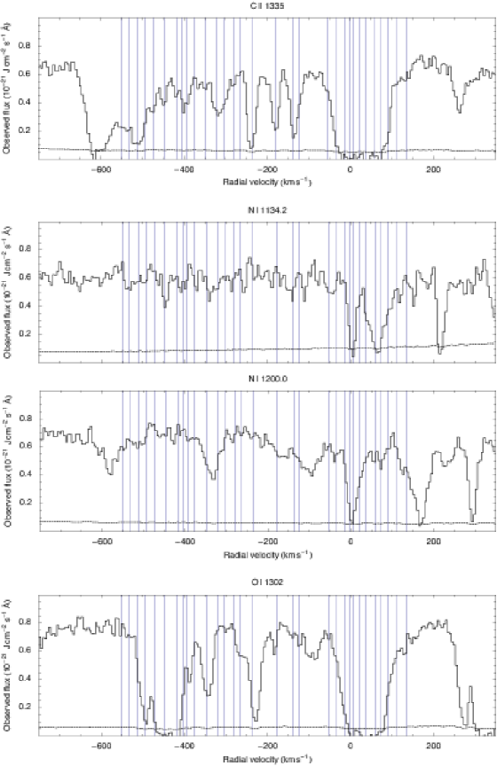
Figure 5: Associated metal lines recorded with the STIS spectrograph. The solid and dashed lines mark the observed flux and its standard deviation, respectively. Positions of associated metal lines found with UVES are indicated by vertical lines. Note that many lines are blended within the Lyman forest

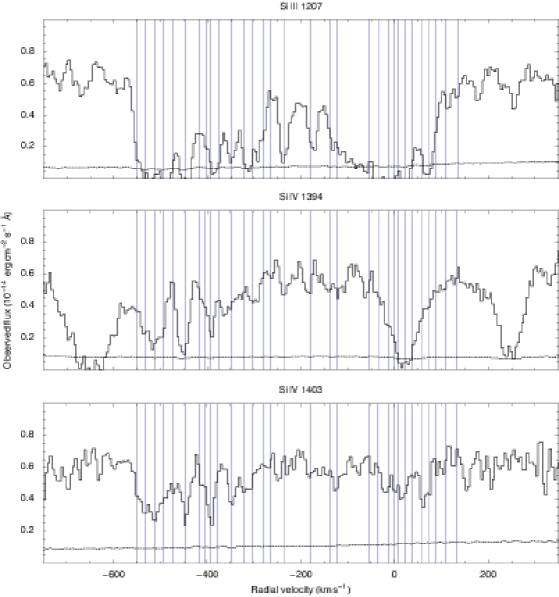
Figure 5: continued.

Immediate evidence of ionized gas is provided by the detection of C iv lines (Fig. 2) and the presence of Si iii and Si iv absorption (see Fig. 5 provided in the Online Material). Apparent column densities of up to $10^{13}$ cm^-2 are found for all high-ions. Except for the broad C iv lines, the velocity structures of low- and high-ion profiles are similar, suggesting a common spatial origin. In particular for components 2-4 the apparent column densities of different Si ions compare, which indicates an H ii region. The apparent optical depths of Si iii and Si iv decreases for components 7-16, whereas the optical depth of Si ii peaks at component 16. The optically thick absorption between components 19 and 20 of the Si iii profile indicates ionization, but Si iii absorption for this velocity interval is not confirmed by the rest of metal lines.

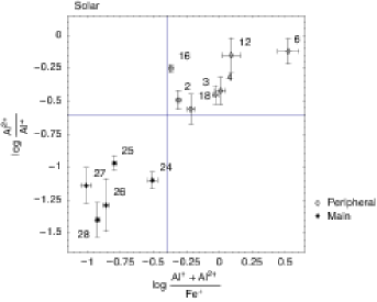
Figure 6: Empirical diagram of ionization vs apparent abundance of Al relative to Fe. Note that the peripheral and main components are well separated

Firm evidence of ionized gas is provided by the column density ratios of Al ii, Al iii, and Fe ii lines. For components 2-4, 6, 12, 16, and 18 the apparent abundance of Al relative to Fe is a factor of 4-30 higher than expected for a neutral medium with solar chemical composition (Fig. 6). The apparent enrichment of Al cannot be explained by the presence of dust because the expected depletion of Al into grains is typically an order of magnitude higher than that of Fe (Spitzer & Jenkins, 1975). On the other hand, Al is produced with $\alpha$-elements which are known to experience a nucleosynthetic history different from that of Fe. For instance, in Galactic thick disk stars the abundance ratio of Al to Fe is found to be enhanced by a factor of 2-4 relative to the solar value (Prochaska et al., 2000). Nonetheless, the apparent enrichment of Al is correlated with the column density ratio of Al iii to Al ii lines, indicating ionization rather than nucleosynthetic enrichment (Fig. 6).

Further confidence is provided by photoionization simulations. For the calculations we consider a plane-parallel slab of gas that is irradiated by the cosmic UV background of QSOs and galaxies (Madau et al., 1999). We further assume a column density of $10^{16}$ hydrogen atoms cm^-2 and solar chemical composition. The photoionization models are defined by the total hydrogen density $n_{\mathrm{H}}$ and the dimensionless ionization parameter

$$U=\frac{n_{\gamma}}{n_{\mathrm{H}}},$$ (1)

where

$$n_{\gamma}=\frac{4\pi}{c}\int_{\nu_{\mathrm{L}}}^{\infty}\frac{J(\nu)}{h\nu}\,\mathrm{d}\nu$$ (2)

is the number density of hydrogen-ionizing photons striking the illuminated face of the slab. For instance, for a total hydrogen density of $n_{\mathrm{H}}=10^{-1}$ particles cm^-3 the cosmic UV background with $4\pi J_{\nu_{\mathrm{L}}}=8.6\times 10^{-21}$ erg cm^-2 corresponds to an ionization parameter of $U=2\times 10^{-4}$. Figure 7 demonstrates that the observed column density ratios are well reproduced, if $U$ falls between $10^{-4}$ and $10^{-3}$. The only exception is the ratio of Mg ii to Mg i, which is overpredicted by a factor of two. The degree of ionization for this range of $U$ is higher than 90 percent. Similar results are obtained for column densities of $10^{17}$ and $10^{18}$ hydrogen atoms cm^-2 and column density ratios corresponding to component 16.

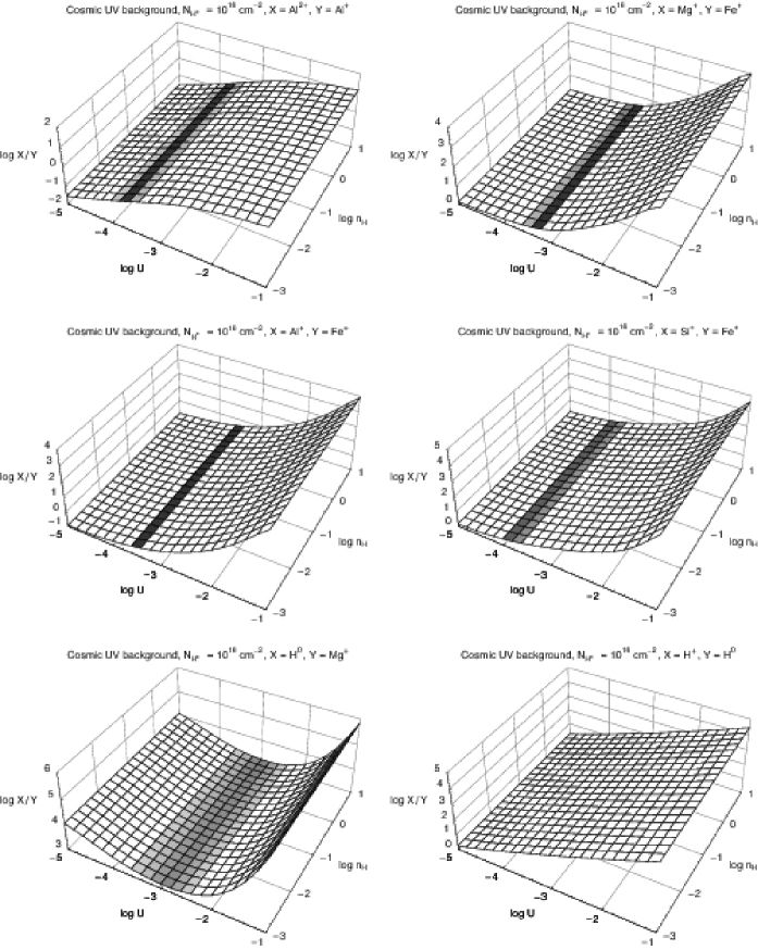
Figure 7: Photoionization simulations considering a plane-parallel slab of gas with column density of $10^{16}$ hydrogen atoms cm^-2 and solar chemical composition. The abscissas mark the ionization parameter $U$ and the total hydrogen density $n_{\mathrm{H}}$. Shaded cells indicate consistency with the observed column density ratios for component 2, unshaded cells mark contradiction at more than 99.7 percent significance. For the medium corresponding to component 2 where $U>10^{-4}$ the predicted degree of ionization exceeds 90 percent. Note that the observed column density ratios do pretend an enrichment of $\alpha$-elements when ionization effects are ignored

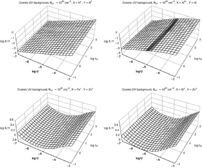
Figure 8: The same as Fig. 7 but a plane parallel slab with column density of $10^{20}$ hydrogen atoms cm^-2 is considered. Top: For a total hydrogen density of $10^{-1}$ particles cm^-3 the cosmic UV background corresponds to an ionization parameter of $U=2\times 10^{-4}$. For denser regions like molecular gas the same ionizing background corresponds to $U<10^{-4}$, implying that at most 10 percent of the hydrogen is ionized. This argument is confirmed by the observed column density ratio of Al ions (illustrated by the shading for component 24, but also see Fig. 6). Bottom: The minimum of the predicted ratio of Fe and Zn ion abundances corresponds to the case where both elements almost completely reside in the first ionization stage and the abundance ratio of ions is almost equal to the (solar) abundance ratio of elements. Note that ionization effects cannot pretend a depletion of Fe relative to Zn. The situation for Si and Zn is similar

In summary, there is conclusive evidence that the peripheral metal line components are formed within H ii regions. An empirical method to identify a H ii region when individual H i components are not detected is provided by Figure 6.

4.2.2 Main components

The presence of ionized gas within the main absorber is not as evident as for the periphery. The Si iii profile is optically thick, suggesting an apparent column density possibly exceeding $10^{13}$ ions cm^-2 for components 20-28, but most of the absorption is due to Lyman forest lines (see the preceding subsection). While the stronger Si iv profile is blended into the Lyman forest, the weaker Si iv profile may confirm the Si iii absorption for components 27-31. Conclusive evidence of ionized gas is provided by the C iv and Al iii lines. The velocity structure of the C iv line, with an apparent column density of up to $2\times 10^{12}$ ions cm^-2, is weak and without noticeable substructure in the domain of components 22-26, indicating that ionized and neutral gas are not intermixed. In contrast, the Al iii profiles indicate a homogenous distribution of high- and low-ions for components 23-25. The column density ratio of Al iii to Al ii lines is less than $1/10$ for all components (Fig. 6).

According to simple photoionization calculations an ionization of the molecular regions due to the cosmic UV background is ruled out (Fig. 8). However, some fractional ionization due to stellar sources is conceivable. The comparison with photoionization simulations considering both interstellar radiation and the formation of molecules and dust requires an accurate recording of H₂ lines that is not available. Our simple attempts assuming Galactic environmental conditions have yielded inconsistent results, which reproduce the column density ratios of Fe i to Fe ii and Si i to Si ii as well as the relative population of neutral carbon fine-structure levels, but both overpredict the amount of molecular hydrogen and underpredict the strength of the Ca ii absorption by more than one order of magnitude. Our calculations hence suggest that the radiation field and the density structure of the absorber are more complex. In fact, for component 23 the neutral species Fe i, Si i and S i have much lower broadening parameters than Fe ii and Si ii, which indicates that the different ionization stages are not formed in the same region. Photoionization calculations without modelling the density structure are therefore meaningless. Similar conclusions have been drawn by D’Odorico (2007) who failed to reproduce the observed Mg i to Mg ii, Fe i to Fe ii and Ca i to Ca ii ratios in a metal line system toward HE 0001-2340.

4.3 Metal abundances and dust depletion

Besides ionization and nucleosynthetic effects, the chemical composition analysis of interstellar environments is hampered by dust grains removing an unknown amount of atoms from the gaseous phase (Spitzer & Jenkins, 1975; Savage & Sembach, 1996). The accepted procedure to unravel these effects is to compare the abundance of refractory and volatile elements $X,Y$ for which the photospheric abundance ratio $(X/Y)$ is constant in stars over a wide range of metallicities. In that case an observed deviation from the stellar ratios is unlikely to have a nucleosynthetic origin. Even though the existence of a stellar proxy for interstellar abundances is questionable (Sofia & Meyer, 2001) the Sun is used as a standard of reference for the total, i.e. gas plus dust, interstellar composition. For given observed column densities $N_{X}$ and $N_{Y}$ the relative abundance of elements $X$ and $Y$ is expressed as

$$[X/Y]=\log(N_{X}/N_{Y})-\log(X/Y)_{\sun}.$$ (3)

Element abundances relative to hydrogen are termed absolute abundances. For chemical composition analysis, we use the metal abundances in meteorites (Anders & Grevesse, 1989) as a standard of reference.

4.3.1 Peripheral components

Since the peripheral components are formed within H ii regions, the element abundances cannot be determined directly. The observed ion abundances, however, are supersolar and photoionization calculations conform with the idea that both absolute and relative metal abundances are solar (Fig. 7).

4.3.2 Main components

For the main components photoionization calculations suggest that the absorbing material is predominantly neutral and ionization effects are negligible, i.e. all elements are accurately represented by the predominant ions. For the chemical composition analysis and the proper unravelling of dust depletion and nucleosynthetic effects the detection of volatile elements is essential. The only volatile element detected in the predominant ionization stage with accurate column density measurements for several main components is Zn. For other volatile elements like N and O also detected in the predominant ionization stage, the absorption is saturated and largely blended with Lyman forest lines (Fig. 5). Even though the Zn ii absorption is weak, the individual column densities are well defined because the positional and broadening parameters of the decomposed Zn ii profiles are tied to those of the Fe ii lines.

Gas-phase abundances

The observed abundances of refractory elements relative to Zn for components 23-28 are illustrated in Fig. 9. For components 23 and 24 the underabundance of the iron group elements Cr, Mn, Fe and Ni relative to Zn is comparable to that in the Galactic warm disk, similar to what has been found by Rodriguez et al. (2006), whereas the mild and even vanishing depletion for components 25 and 28 is not found in Galactic interstellar space (Spitzer & Jenkins, 1975; Savage & Sembach, 1996). The relative abundances found for components 26 and 27 rather resemble those of the Galactic halo. If Zn is indeed undepleted and traces Fe as found by Nissen et al. (2004), the pattern of relative abundances directly reflects the differential depletion of chemical elements into dust grains. This idea gains indirect support by the detection of H₂ absorption lines associated with components 23 and 24, since molecules are essentially formed on the surface of dust grains (Cazaux et al., 2005; Williams, 2005). For all components showing evidence of dust grains, the depletion of Si is stronger than in the Galactic warm disk, but weaker than in the cold disk. For all but the H₂-bearing components Mn is systematically underabundant when compared to the rest of iron group elements. The synthesis of Mn, however, is expected to be suppressed due to the nuclear odd-even effect. The average metallicity for components 23-28 is $[\mathrm{Zn}/\mathrm{H}]=-0.38\pm 0.04$.

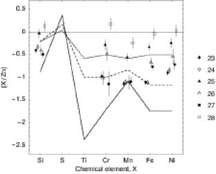
Figure 9: Gas-phase abundance ratios (relative to solar ratios) for the main components 23-28 compared with those in the Galactic interstellar medium (dotted line: warm halo gas; dashed line: warm disk gas; solid line: cold disk gas; Welty et al., 2001). If the volatile element Zn is undepleted, the abundance ratios reflect the differential depletion of chemical elements into dust grains. Note that Cr, Mn, Fe, and Ni are strongly depleted for the H₂-bearing components 23 and 24, but essentially undepleted for component 28

The apparent underabundance of Fe (and Si) relative to Zn cannot be the result of ionization effects caused by the cosmic UV background since these would pretend an enhanced abundance (Fig. 8). Therefore, the interpretation of the observed underabundance as evidence of depletion into dust grains cannot be questioned without admitting very unusual nucleosynthetic effects. On the other hand, if the observed underabundance of Fe (and Si) relative to Zn is the net result of dust depletion and ionization effects, the true depletion might be even stronger than illustrated in Fig. 9.

In summary, there is decisive evidence of Galaxy-like differential depletion of elements into dust grains, with a significant gradient from component to component as if the sight line is intersecting different interstellar environments comparable to the Galactic disk and halo. Another such example may be the DLA system toward the gravitationally lensed QSO HE 0512–3329, where different element abundances are detected along two lines of sight (Lopez et al., 2005). Further examples are given by Dessauges-Zavadsky et al. (2006).

Dust correction

Based on the presumption that the chemical composition of dust is defined by the physical state and the chemical composition of the medium, Vladilo (2002b, a) has worked out an analytic relation between the dust depletion patterns for interstellar environments of different types. Though generalizing former approaches where the dust composition is assumed to be constant, his new approach still implies that the dust composition does not depend on the history of the medium, a condition that is not strictly satisfied since the formation of dust and ices involves irreversible processes (Vidali et al., 2005).

For any interstellar environments $i,j$ and constant sensitivity of the chemical composition of dust to variations in the dust-to-metal ratio $\rho$ and the chemical composition of the medium, the fractions of the generic and reference elements $X,Y$ contained in dust grains are related by

$$f_{X,j}=\rho^{\eta_{X}+1}10^{[X/Y]_{\mathrm{m},j}\,(\epsilon_{X}-1)}f_{X,i}.$$ (4)

The subscript ‘m’ indicates reference to all atoms in the medium, i.e. in the gaseous and the solid phase. The exponents $\eta_{X},\epsilon_{X}$ define the response of the relative abundance of $X$ in the solid phase to the variation of the fraction of $Y$ contained in dust, and the relative abundance of $X$ in the medium, respectively (Vladilo, 2002b, a).

Equation (4) is capable of reproducing the Galactic interstellar depletion patterns $\delta_{X}=\log(1-f_{X})$ with a varying dust-to-metal ratio

$$\rho=\frac{f_{Y,j}}{f_{Y,i}}$$ (5)

and a single set of empirical constants $(f_{X,i},\eta_{X})$. The depletion patterns in the interstellar medium of the SMC can be reproduced with the same set of constants, if the relative element abundances are allowed to deviate from solar values. From the theoretical point of view, the dust-corrected element abundances of high-redshift DLA systems show better consistency with galactic chemical evolution models than the plain observations (Calura et al., 2003).

An explicit relation between observed and intrinsic absolute abundances is obtained by using Eq. (4) to express the fraction of $X$ contained in the gaseous phase of medium $j$:

$$\frac{10^{[X/\mathrm{H}]_{\mathrm{g},j}}}{10^{[X/\mathrm{H}]_{\mathrm{m},j}}}=1-\rho^{\eta_{X}+1}10^{[X/Y]_{\mathrm{m},j}\,(\epsilon_{X}-1)}f_{X,i},$$ (6)

where the subscript ‘g’ indicates reference atoms in the gaseous phase. The parameters $f_{X,i}$ and $\eta_{X}$ can be calculated from Galactic interstellar depletion patterns (Vladilo, 2002b, a), whereas the dust-to-gas ratio $\rho$ is an implicit function of the observed and intrinsic abundance ratios

$$\rho-\frac{10^{[X/Y]_{\mathrm{m},j}\,\epsilon_{X}}f_{X,i}}{10^{[X/Y]_{\mathrm{g},j}}f_{Y,i}}\rho^{\eta_{X}+1}+\frac{10^{[X/Y]_{\mathrm{m},j}}-10^{[X/Y]_{\mathrm{g},j}}}{10^{[X/Y]_{\mathrm{g},j}}f_{Y,i}}=0,$$ (7)

which is obtained by dividing Eq. (6) by the corresponding equation for $X=Y$. The intrinsic abundance ratio $[X/Y]_{\mathrm{m},j}$ and the exponent $\epsilon_{X}$ are unknown parameters. For the latter only two extreme cases are considered where the relative element abundances in the solid phase and the medium are mutually independent, $\epsilon_{X}=0$, or directly proportional, $\epsilon_{X}=1$. Superlinear response $\epsilon_{X}>1$ is ignored. For the intrinsic abundance ratio $[X/Y]_{\mathrm{m},j}$ an element $X=Z$ ideally tracing the reference element $Y$ is required.

Given the observed abundance ratios $10^{[X/Y]_{\mathrm{g},j}}$ and an educated guess of $[Z/Y]_{\mathrm{m},j}$, the dust-to-metal ratio $\rho$ is defined by Eq.(7). The rest of intrinsic abundance ratios $[X/Y]_{\mathrm{m},j}$ for elements $X\neq Z$ implicitly follows from

$$10^{[X/Y]_{\mathrm{m},j}}-\rho^{\eta_{X}+1}f_{X,i}\,10^{[X/Y]_{\mathrm{m},j}\,\epsilon_{X}}+(\rho f_{Y,i}-1)\,10^{[X/Y]_{\mathrm{g},j}}=0.$$ (8)

The roots of Eqs. (7, 8) can be calculated with simple bisectioning and the statistical errors of all quantities involved in the calculation, i.e. observed column densities, meteoritic element abundances, $f_{X,i}$, $\eta_{X}$, can be propagated by means of Monte Carlo methods. The intrinsic absolute element abundances $[X/\mathrm{H}]_{\mathrm{m},j}$ follow from Eq. (6). The dust-to-gas ratio is given by

$$\kappa=\rho\,10^{[Y/\mathrm{H}]_{\mathrm{m},j}}.$$ (9)

For the corrective procedure we choose $Y=\mathrm{Fe}$ since the Fe ii lines provide the most reliable column densities. The most suitable element for calculating the dust-to-metal ratio is $Z=\mathrm{Zn}$. The rest of elements with known parameters $f_{X,i},\eta_{X}$ are either too affine to the solid state, or have an interstellar enrichment history too different from that of Fe to make an assumption about the intrinsic abundance ratio. If Zn proves a tracer of Si as suggested by Wolfe et al. (2005), the combination $Y=\mathrm{Si}$ and $Z=\mathrm{Zn}$ will be an eligible option. For the present case, however, this option results in implausible dust-to-metal ratios throughout exceeding those in the Galactic cold disk. Following Vladilo (2004), we consider six different model cases labeled with A0, A1, B0, B1, E0, and E1. The capital letter indicates the intrinsic abundance of Zn relative to Fe, assumed solar for cases A and B, and enhanced for case E, $[\mathrm{Zn}/\mathrm{Fe}]_{\mathrm{m},j}=0.1$. For cases A and E the fraction of Zn assumed to be contained in interstellar dust is $f_{\mathrm{Zn},i}=0.59$, for case B the assumed depletion is lower, $f_{\mathrm{Zn},i}=0.30$. The number to the right of the capital letter directly represents the value of the exponent $\epsilon_{X}$. Zinc might be no precise tracer of iron since its exact nucleosynthetic origin is unknown, but the average photospheric abundance ratios in Galactic disk and halo stars are approximately solar or slightly enhanced (Chen et al., 2004; Nissen et al., 2004) and substantiate the model specifications.

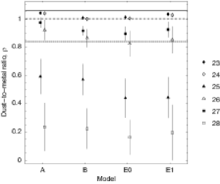
Figure 10: Dust-to-metal ratio $\rho$ for the main components 23-28 compared with values typical for the Galactic interstellar medium (dotted line: warm halo gas; dashed line: warm disk gas; solid line: cold disk gas; Vladilo, 2002a). The results for models A and B do not depend on the exponent $\epsilon_{X}$

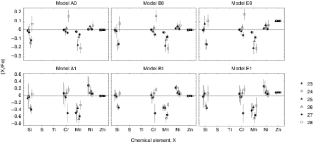
Figure 11: Intrinsic abundance ratios (relative to solar ratios) for the main components 23-28

Dust-to-metal ratio

The calculated dust-to-metal ratios and corresponding fractions of Fe contained in dust are presented in Fig. 10 and Table 4, respectively. If there is a one-to-one correspondence between the physical state of the interstellar environment and the dust-to-metal ratio, Fig. 10 illustrates the multiphase structure of the absorbing medium. Though such diversified structure is characteristic for the interstellar medium in the Galaxy and the Magellanic Clouds (Savage & Sembach, 1996; Welty et al., 1997, 1999, 2001) it is usually not attributed to DLA systems (Prochaska, 2003). The dust-to-metal ratio for the H₂-bearing components 23 and 24 exceeds the ratio of the warm Galactic disk, for some models the ratio approaches the ratio found in the cold disk. For components 26 and 27 the dust-to-metal ratio compares to that in the intermediate warm Galactic disk and halo, whereas for the the rest of components the dust-to-metal ratio is typical of higher-redshift DLA systems (Vladilo, 2004). These basic results conform with the observed depletion pattern (Fig. 9) and are independent of the adopted model, in particular unaffected by the choice of $[\mathrm{Zn}/\mathrm{Fe}]_{\mathrm{m},j}$.

Intrinsic abundances and dust-to-gas ratio

The calculated intrinsic abundance ratios are presented in Fig. 11. For all models the intrinsic abundance ratios conform with solar values, apart from three exceptions:

1. The mean intrinsic abundance of Ni relative to Fe is slightly enhanced. Similar offsets are also found for Galactic thick disk stars (Prochaska et al., 2000).

2. The intrinsic abundance of Mn is reduced. The reduction is most distinct for the less dust-containing components 25-28 and for models where the relative element abundances in dust and in the medium scale directly, i.e. $\eta_{X}=1$. Similar underabundances, usually attributed to the nuclear odd-even effect, are found for Galactic thick disk stars (Prochaska et al., 2000) as well as DLA systems (Dessauges-Zavadsky et al., 2006).

3. For the intermediate components 26 and 27 the intrinsic abundance of Si relative to Fe is always subsolar, in marked contrast to the expected nucleosynthetic enrichment of $\alpha$-elements and to element abundances found for Galactic stars. For these components, the dust-corrective procedure may have overestimated (underestimated) the fraction of Fe (Si) contained in dust.

Table 4: Fractions of Fe contained in dust, $f_{\mathrm{Fe},j}$, for the main components 23-28 and different models. The results for models A and B do not depend on the exponent $\epsilon_{X}$

No.	A	B	E0	E1	Mean
23	$0.98\pm 0.01$	$0.95\pm 0.01$	$0.95\pm 0.01$	$0.97\pm 0.01$	$0.96\pm 0.02$
24	$0.98\pm 0.01$	$0.94\pm 0.01$	$0.94\pm 0.01$	$0.96\pm 0.01$	$0.96\pm 0.02$
25	$0.56\pm 0.12$	$0.54\pm 0.10$	$0.41\pm 0.13$	$0.42\pm 0.14$	$0.48\pm 0.08$
26	$0.86\pm 0.07$	$0.81\pm 0.06$	$0.77\pm 0.08$	$0.80\pm 0.09$	$0.81\pm 0.04$
27	$0.92\pm 0.03$	$0.86\pm 0.03$	$0.84\pm 0.05$	$0.87\pm 0.05$	$0.87\pm 0.03$
28	$0.22\pm 0.16$	$0.21\pm 0.13$	$0.15\pm 0.11$	$0.18\pm 0.18$	$0.19\pm 0.03$

Table 5: Cumulative dust-corrected column density of Fe contained in the main absorber, $\log N_{\mathrm{Fe},\mathrm{m}}$ (cm^-2)

No.	A	B	E0	E1	Mean
23-24	$15.44\pm 0.18$	$15.00\pm 0.04$	$15.03\pm 0.05$	$15.28\pm 0.14$	$15.19\pm 0.21$
23-28	$15.54\pm 0.17$	$15.15\pm 0.03$	$15.16\pm 0.04$	$15.39\pm 0.18$	$15.31\pm 0.19$

Since only the total column density of hydrogen atoms contained in the main absorber is known, Eq. (6) cannot be used to calculate the intrinsic absolute abundances for individual components. Nonetheless, by cumulating the individual dust-corrected column densities $N_{Y,\mathrm{m}}=\sum_{j}N_{Y,j}/(1-f_{Y,j})$, we can calculate an average intrinsic metallicity $[Y/\mathrm{H}]_{\mathrm{m}}$. Inserting the calculated fractions of Fe contained in dust (Table 5) yields an almost solar intrinsic metallicity of $[\mathrm{Fe}/\mathrm{H}]_{\mathrm{m}}=-0.08\pm 0.19$. Assuming that the observed H i absorption is only constituted by components 23-24, the dust-to-metal ratio of $\rho=1.02\pm 0.02$ and the intrinsic metallicity of $[\mathrm{Fe}/\mathrm{H}]_{\mathrm{m}}=-0.20\pm 0.21$ give an average dust-to-gas ratio of $\kappa=0.64\pm 0.31$.

4.4 Kinematic structure

With an absorption velocity interval extending for $700$ km s^-1 the kinematic distribution of associated metal line components is quite unique. Only the $z=1.97$ DLA system toward QSO 0013–004 shows an even more extended spread (Petijean et al., 2002). The $z=2.19$ sub-DLA system toward HE 0001–2340 has a comparable neutral hydrogen column density, but a less extended absorption velocity interval of $400$ km s^-1 and much lower metallicity (Richter et al., 2005). Rotating disks models (Prochaska & Wolfe, 1997) and simulations of merging protogalactic clumps (Haehnelt et al., 1998) do explain the characteristic kinematic features like asymmetric edge-leading line profiles, but fail to reproduce absorption intervals exceeding $250$ km s^-1. Large absorption intervals have therefore been associated with interacting or merging galaxies producing extended tidal filaments like the Antennae (e.g. Wilson et al., 2000; Zhang et al., 2001). Another viable scenario is a line-of-sight intercepting a cluster of galaxies. The kinematic distribution of metal line components associated with the present sub-DLA system (Fig. 2) indeed supports the idea that two different absorbers are involved.

4.4.1 Peripheral components

The peripheral components show markedly different characteristics. For the velocity region from $-560$ to $-260$ km ^-1 the average number density of components is about one component per $20$ km s^-1. The dominating substructure is edge-leading, but the remaining features appear randomly distributed. In contrast, the velocity region from $-260$ to $-60$ km s^-1 includes only four components, which are arranged in three isolated groups.

4.4.2 Main components

The main structure is characterized by the highest frequency of peaks, with an average of one peak every $15$ km s^-1. Two substructures may be recognized, both edge-leading for the less refractory elements like Mg and Si, but rather unordered otherwise.

Particularly instructive is the comparison of extragalactic Ca ii absorption lines with those originating in the Galactic halo (Bowen, 1991). First ignoring components 23 and 24, the redshifted and the Galactic line profiles are remarkably similar (Fig. 4), indicating that components 25-28 correspond to halo-like structures. Further developing this analogy, the narrow structures 23 and 24 not present in the absorption by the Galactic halo may be interpreted as signature of disk-like agglomeration, a picture which conforms with the observed depletion of elements into dust (Figs. 9, 10).

4.5 Physical conditions

The physical conditions in DLA absorbers like the number density and kinetic temperature of hydrogen atoms and the local microwave and FUV radiation can be inferred from the diagnostics of fine-structure absorption lines (Bahcall & Wolf, 1968; Silva & Viegas, 2002). For the present absorber the analysis of excited C i lines associated with the H₂ bearing components 23 and 24 provides an upper limit on the FUV input (Quast et al., 2002). The study of H₂ lines predicts a radiation input exceeding the Galactic interstellar energy density by more than an order of magnitude and a number density greater than 100 hydrogen atoms cm^-2 (Reimers et al., 2003; Hirashita & Ferrara, 2005).

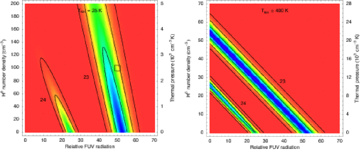
Figure 12: Physical conditions for the H₂-bearing components 23 and 24 inferred from the observed population of C⁰ fine-structure levels. Contour lines are drawn at 0.61, 0.14, and 0.01 of the maximum probability density and would correspond to the boundaries of the 68.3, 95.4, and 99.7 percent confidence regions if the distributions were normal. Two extreme cases are considered for the kinetic gas temperature. Left: The high number density of hydrogen atoms and the intense FUV radiation found by Hirashita & Ferrara (2005, marked by an empty square) require a low kinetic temperature. Right: If the population of lower and higher rotational H₂ levels is in thermal equilibrium with $T_{\mathrm{kin}}=400$ K, either an intense FUV field or a high number density is ruled out

Assuming an FUV input equal to the scaled generic Galactic radiation field (Draine & Bertoldi, 1996), but otherwise repeating the statistical equilibrium calculations of Quast et al. (2002), we note that both an intense radiation field and a number density exceeding 100 hydrogen atoms cm^-2 only conform with the observed population of fine-structure levels, if the kinetic temperature is about $T_{\mathrm{kin}}=25$ K, which is different from the population temperature of $80$ K inferred from the lower rotational H₂ levels (Reimers et al., 2003). On the other hand, if the population of lower and higher rotational H₂ levels is in thermal equilibrium with $T_{\mathrm{kin}}=400$ K, the number density of hydrogen atoms can only exceed $60$ cm^-2 if the local and Galactic interstellar radiation are comparable (Fig. 12). The present spectroscopy of H₂ lines, however, is too inadequate to provide reliable results. Besides, the spatial distributions of carbon atoms and hydrogen molecules may not be identical, allowing different kinetic temperatures for both constituents (Spitzer & Jenkins, 1975). DLA systems where the population of lower and higher rotational $H_{2}$ levels are not in thermal equilibrium and shielding effects are likely to play an improtant role have been investigated by Noterdaeme et al. (2007a, b).

5 Summary and conclusions

Based on high-resolution spectra obtained with STIS and the VLT UVES we have presented a reanalysis of the chemical composition, kinematic structure, and physical conditions of the H₂-bearing sub-DLA system toward HE 0515–4414. The sub-damped system is unusual in several aspects:

1. The velocity interval of associated metal lines extends for $700$ km s^-1. The velocity distribution of metal line components is bimodal, indicating the presence of two interacting absorbers.

2. Most of the associated metal line components are formed within H ii regions, only one third of the components associated with the predominantly neutral main absorber.

3. For the main components 23-28 the observed abundance ratios of refractory elements Si, Cr, Mn Fe, Ni to Zn show a distinct gradient along the sight line. The differential depletion of refractory elements ranges from Galactic warm disk to halo-like and essentially undepleted patterns. The variation in the dust-to-metal ratio indicates the multiphase structure of the absorbing medium. The dust-corrected metal abundances show the nucleosynthetic odd-even effect and might imply an anomalous depletion of Si relative to Fe, but otherwise do correspond to solar abundance ratios. The intrinsic average metallicity is almost solar, $[\mathrm{Fe}/\mathrm{H}]_{\mathrm{m}}=-0.08\pm 0.19$, whereas the uncorrected average is $[\mathrm{Zn}/\mathrm{H}]_{\mathrm{g}}=-0.38\pm 0.04$. For the H₂-bearing components 23 and 24 the dust-to-metal and dust-to-gas ratios (relative to Galactic warm disk ratios) are $\rho=1.02\pm 0.02$ and $\kappa=0.64\pm 0.31$, respectively. The ion abundances in the periphery conform with solar element composition.

4. The diagnostics of fine-structure lines is not conclusive. Adequate recordings of the H₂ lines are needed to provide reliable results.

The presence of H ii regions might have consequences for the DLA abundance diagnostics in general. If any metal line components are connected with H ii rather than H i regions, the usual averaging of element abundances is incorrect. In particular, ionization effects can pretend an enrichment of $\alpha$ elements. We have obtained a diagnostic diagram (Fig. 6) which allows to detect H ii region-like ionization conditions from empirical Al ii, Al iii, and Fe ii column densities. If both $N_{Al\textsc{iii}}/N_{Al\textsc{ii}}>0.25$ and $N_{\mathrm{Al}}/N_{Fe\textsc{ii}}>0.40$, the absorbing material is largely ionized. In this context, it is interesting to note that high column densities can be attained by the interception of relatively compact regions. For the present case Reimers et al. (2003) have already pointed out that the absorption path length contributed by the H₂-bearing components 23 and 24 is less than 1 lyr when the number density of hydrogen atoms is about $100$ cm^-3.

Our analysis shows that sub-DLA systems can exhibit solar metallicities. If the highest-metallicity sub-DLA absorbers prove to be regular DLA absorbers having consumed large amounts of neutral hydrogen due to massive star formation, their detection is important. Modern surveys of DLA systems setting the cut-off below the traditional column density limit may provide interesting insights.

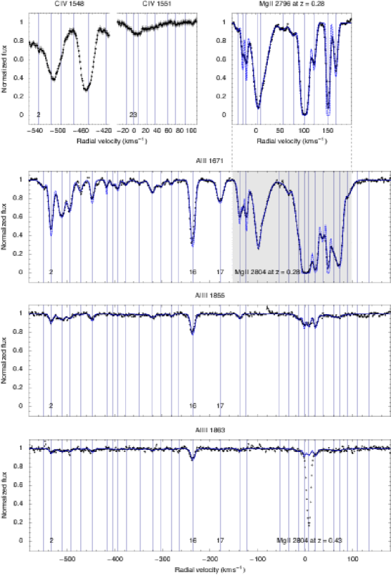
Figure 2: continued. Note that the Al ii profile is blended with an Mg ii ensemble at redshift $z=0.28$. Blended parts of the C iv profiles are omitted for convenience

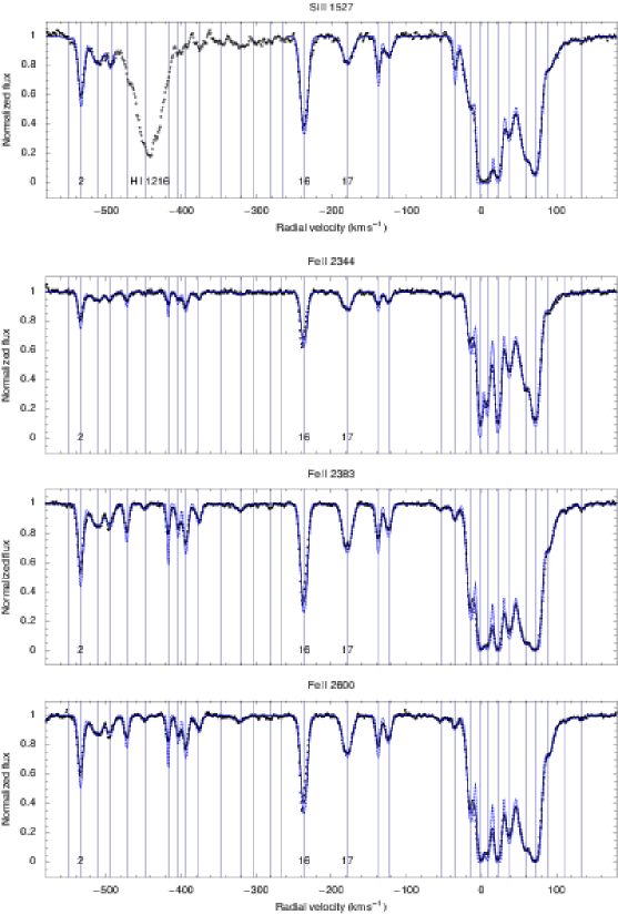
Figure 2: continued.

[x]@llllll@ Optimized decomposition of the metal lines shown in Figs. 2 and 3
No. Transitions $\phantom{-}\mathrm{RV}$ (km s^-1) $b$ (km s^-1) $\log N$ (cm^-2)
continued.
No. Transitions $\phantom{-}\mathrm{RV}$ (km s^-1) $b$ (km s^-1) $\log N$ (cm^-2)
1 Mg ii 2796, 2804 $-550.20\pm 0.15$ $6.59\pm 0.25$ $11.79\pm 0.02$
1 Al ii 1671 $-550.20$ $7.26\pm 1.39$ $11.17\pm 0.08$
1 Si ii 1527, 1808 $-550.20\pm 0.15$ $6.59\pm 0.25$ $11.61\pm 0.30$

2 Mg i 2026, 2853 $-533.51\pm 0.03$ $5.21\pm 0.34$ $11.08\pm 0.02$
2 Mg ii 2796, 2804 $-533.51\pm 0.03$ $5.12\pm 0.05$ $12.90\pm 0.01$
2 Al ii 1671 $-533.5$ $4.79\pm 0.25$ $12.00\pm 0.01$
2 Al iii 1855, 1863 $-533.5$ $4.79\pm 0.25$ $11.51\pm 0.07$
2 Si ii 1527, 1808 $-533.51\pm 0.03$ $4.45\pm 0.37$ $12.97\pm 0.03$
2 Fe ii 1608, 2344, 2374, 2383, 2587, 2600 $-533.51\pm 0.03$ $3.73\pm 0.10$ $12.43\pm 0.01$

3 Mg i 2026, 2853 $-511.33\pm 0.07$ $\phantom{0}9.24\pm 0.75$ $10.94\pm 0.04$
3 Mg ii 2796, 2804 $-511.33\pm 0.07$ $\phantom{0}9.96\pm 0.14$ $12.83\pm 0.01$
3 Al ii 1671 $-511.33$ $10.03\pm 0.45$ $12.08\pm 0.01$
3 Al iii 1855, 1863 $-511.33$ $10.03\pm 0.45$ $11.63\pm 0.07$
3 Si ii 1527, 1808 $-511.33\pm 0.07$ $11.20\pm 1.53$ $12.89\pm 0.05$
3 Fe ii 1608, 2344, 2374, 2383, 2587, 2600 $-511.33\pm 0.07$ $11.06\pm 0.33$ $12.24\pm 0.01$

4 Mg i 2026, 2853 $-493.59\pm 0.08$ $6.86\pm 0.85$ $10.76\pm 0.05$
4 Mg ii 2796, 2804 $-493.59\pm 0.08$ $6.80\pm 0.12$ $12.53\pm 0.01$
4 Al ii 1671 $-493.59$ $6.00\pm 0.46$ $11.73\pm 0.03$
4 Al iii 1855, 1863 $-493.59$ $6.00\pm 0.46$ $11.31\pm 0.10$
4 Si ii 1527, 1808 $-493.59\pm 0.08$ $5.43\pm 1.36$ $12.61\pm 0.08$
4 Fe ii 1608, 2344, 2374, 2383, 2587, 2600 $-493.59\pm 0.08$ $5.06\pm 0.29$ $11.86\pm 0.02$

5 Mg i 2026, 2853 $-472.09\pm 0.06$ $6.88\pm 0.81$ $10.62\pm 0.05$
5 Mg ii 2796, 2804 $-472.09\pm 0.06$ $5.24\pm 0.13$ $12.19\pm 0.01$
5 Al ii 1671 $-472.09$ $6.36\pm 0.91$ $11.29\pm 0.06$
5 Al iii 1855, 1863 $-472.09$ $6.36\pm 0.91$ $10.36\pm 0.69$
5 Fe ii 1608, 2344, 2374, 2383, 2587, 2600 $-472.09\pm 0.06$ $3.12\pm 0.19$ $11.92\pm 0.02$

6 Mg i 2026, 2853 $-447.00\pm 0.08$ $6.54\pm 0.87$ $10.50\pm 0.06$
6 Mg ii 2796, 2804 $-447.00\pm 0.08$ $7.30\pm 0.13$ $12.29\pm 0.01$
6 Al ii 1671 $-447.00$ $4.46\pm 0.44$ $11.47\pm 0.03$
6 Al iii 1855, 1863 $-447.00$ $4.46\pm 0.44$ $11.35\pm 0.09$
6 Fe ii 1608, 2344, 2374, 2383, 2587, 2600 $-447.00\pm 0.08$ $3.81\pm 1.21$ $11.19\pm 0.07$

7 Mg i 2026, 2853 $-416.85\pm 0.06$ $5.00\pm 1.18$ $10.43\pm 0.08$
7 Mg ii 2796, 2804 $-416.85\pm 0.06$ $3.29\pm 0.17$ $11.87\pm 0.01$
7 Al ii 1671 $-416.85$ $1.88\pm 1.45$ $10.85\pm 0.10$
7 Fe ii 1608, 2344, 2374, 2383, 2587, 2600 $-416.85\pm 0.06$ $1.72\pm 0.20$ $11.91\pm 0.02$

8 Mg ii 2796, 2804 $-403.63\pm 0.09$ $2.63\pm 0.22$ $11.78\pm 0.02$
8 Al ii 1671 $-403.63$ $4.68\pm 1.96$ $10.87\pm 0.12$
8 Al iii 1855, 1863 $-403.63$ $4.68\pm 1.96$ $10.48\pm 0.27$
8 Fe ii 1608, 2344, 2374, 2383, 2587, 2600 $-403.63\pm 0.09$ $2.82\pm 0.34$ $11.81\pm 0.02$

9 Mg i 2026, 2853 $-393.26\pm 0.08$ $6.02\pm 0.93$ $10.58\pm 0.07$
9 Mg ii 2796, 2804 $-393.26\pm 0.08$ $5.56\pm 0.21$ $12.15\pm 0.01$
9 Al ii 1671 $-393.26$ $3.81\pm 1.33$ $11.04\pm 0.08$
9 Al iii 1855, 1863 $-393.26$ $3.81\pm 1.33$ $10.66\pm 0.30$
9 Fe ii 1608, 2344, 2374, 2383, 2587, 2600 $-393.26\pm 0.08$ $3.63\pm 0.19$ $12.13\pm 0.01$

10 Mg ii 2796, 2804 $-376.31\pm 0.13$ $6.02\pm 0.26$ $11.80\pm 0.02$
10 Al ii 1671 $-376.31$ $5.41\pm 1.72$ $10.83\pm 0.12$
10 Al iii 1855, 1863 $-376.31$ $5.41\pm 1.72$ $10.70\pm 0.30$
10 Fe ii 1608, 2344, 2374, 2383, 2587, 2600 $-376.31\pm 0.13$ $4.37\pm 0.24$ $11.77\pm 0.02$

11 Mg ii 2796, 2804 $-347.31\pm 0.23$ $8.56\pm 0.38$ $11.64\pm 0.02$
11 Al ii 1671 $-347.31$ $8.36\pm 4.21$ $10.85\pm 0.15$
11 Al iii 1855, 1863 $-347.31$ $8.36\pm 4.21$ $10.80\pm 0.37$

12 Mg ii 2796, 2804 $-320.68\pm 0.11$ $7.41\pm 0.22$ $12.07\pm 0.01$
12 Al ii 1671 $-320.68$ $7.41\pm 0.95$ $11.41\pm 0.05$
12 Al iii 1855, 1863 $-320.68$ $7.41\pm 0.95$ $11.26\pm 0.12$
12 Fe ii 1608, 2344, 2374, 2383, 2587, 2600 $-320.68\pm 0.11$ $7.80\pm 0.70$ $11.55\pm 0.04$

13 Mg ii 2796, 2804 $-303.41\pm 0.32$ $6.59\pm 0.43$ $11.44\pm 0.03$
13 Al ii 1671 $-303.41$ $7.34\pm 1.39$ $11.11\pm 0.09$
13 Al iii 1855, 1863 $-303.41\pm 0.32$ $7.34\pm 1.39$ $10.64\pm 0.30$

14 Mg ii 2796, 2804 $-280.56\pm 0.15$ $3.19\pm 0.31$ $11.46\pm 0.02$
14 Al ii 1671 $-280.56$ $4.45\pm 1.37$ $10.73\pm 0.11$
14 Al iii 1855, 1863 $-280.56$ $4.45\pm 1.37$ $10.87\pm 0.20$

15 Mg ii 2796, 2804 $-265.46\pm 0.38$ $4.31\pm 0.71$ $11.11\pm 0.05$

16 Mg i 2026, 2853 $-236.14\pm 0.02$ $6.04\pm 0.26$ $11.20\pm 0.02$
16 Mg ii 2796, 2804 $-236.14\pm 0.02$ $6.25\pm 0.04$ $13.23\pm 0.01$
16 Al ii 1671 $-236.14$ $5.72\pm 0.15$ $12.22\pm 0.01$
16 Al iii 1855, 1863 $-236.14$ $5.72\pm 0.15$ $11.97\pm 0.03$
16 Si ii 1527, 1808 $-236.14\pm 0.02$ $5.95\pm 0.17$ $13.33\pm 0.01$
16 Fe ii 1608, 2344, 2374, 2383, 2587, 2600 $-236.14\pm 0.02$ $5.09\pm 0.06$ $12.78\pm 0.01$

17 Mg i 2026, 2853 $-178.49\pm 0.05$ $6.60\pm 0.57$ $10.74\pm 0.04$
17 Mg ii 2796, 2804 $-178.49\pm 0.05$ $8.44\pm 0.09$ $12.51\pm 0.01$
17 Al ii 1671 $-178.49$ $8.28\pm 0.47$ $11.73\pm 0.02$
17 Al iii 1855, 1863 $-178.49$ $8.28\pm 0.47$ $10.66\pm 0.30$
17 Si ii 1527, 1808 $-178.49\pm 0.05$ $9.04\pm 0.47$ $12.80\pm 0.03$
17 Fe ii 1608, 2344, 2374, 2383, 2587, 2600 $-178.49\pm 0.05$ $7.77\pm 0.13$ $12.44\pm 0.01$

18 Mg i 2026, 2853 $-137.31\pm 0.04$ $2.74\pm 0.86$ $10.44\pm 0.06$
18 Mg ii 2796, 2804 $-137.31\pm 0.04$ $3.89\pm 0.08$ $12.44\pm 0.01$
18 Al ii 1671 $-137.31$ $3.96\pm 0.36$ $11.74\pm 0.02$
18 Al iii 1855, 1863 $-137.31$ $3.96\pm 0.36$ $11.18\pm 0.11$
18 Si ii 1527, 1808 $-137.31\pm 0.04$ $3.07\pm 0.35$ $12.62\pm 0.03$
18 Fe ii 1608, 2344, 2374, 2383, 2587, 2600 $-137.31\pm 0.04$ $3.12\pm 0.16$ $12.06\pm 0.01$

19 Mg i 2026, 2853 $-123.63\pm 0.07$ $5.39\pm 3.06$ $10.20\pm 0.11$
19 Mg ii 2796, 2804 $-123.63\pm 0.07$ $5.01\pm 0.13$ $12.18\pm 0.01$
19 Al ii 1671 $-123.63$ $3.48\pm 0.75$ $11.41\pm 0.05$
19 Si ii 1527, 1808 $-123.63\pm 0.07$ $6.55\pm 0.58$ $12.54\pm 0.05$
19 Fe ii 1608, 2344, 2374, 2383, 2587, 2600 $-123.63\pm 0.07$ $4.49\pm 0.22$ $12.01\pm 0.02$

20 Fe ii 1608, 2344, 2374, 2383, 2587, 2600 $-53.77\pm 0.52$ $6.38\pm 0.84$ $11.45\pm 0.05$

21 Mg i 2026, 2853 $-35.06\pm 0.16$ $6.32\pm 1.56$ $10.53\pm 0.07$
21 Al ii 1671 $-35.06$ $6.19\pm 1.02$ $11.29\pm 0.06$
21 Al iii 1855, 1863 $-35.06$ $6.19\pm 1.02$ $10.11\pm 1.37$
21 Si ii 1527, 1808 $-35.06\pm 0.16$ $2.76\pm 0.38$ $12.56\pm 0.04$
21 Fe ii 1608, 2344, 2374, 2383, 2587, 2600 $-35.06\pm 0.16$ $5.08\pm 0.45$ $11.75\pm 0.03$

22 Mg i 2026, 2853 $-13.53\pm 0.07$ $8.52\pm 0.51$ $11.23\pm 0.02$
22 Al ii 1671 $-13.53$ $7.98\pm 0.37$ $12.16\pm 0.02$
22 Al iii 1855, 1863 $-13.53$ $7.98\pm 0.37$ $11.50\pm 0.08$
22 Si ii 1527, 1808 $-13.53\pm 0.07$ $9.97\pm 0.24$ $13.36\pm 0.01$
22 Ca ii 3935 $-13.53\pm 0.07$ $7.89\pm 0.97$ $11.16\pm 0.04$
22 Fe ii 1608, 2344, 2374, 2383, 2587, 2600 $-13.53\pm 0.07$ $5.79\pm 0.10$ $12.90\pm 0.01$

23 Mg i 2026, 2853 $-1.61\pm 0.03$ $2.16\pm 0.05$ $12.41\pm 0.03$
23 Al ii 1671 $-1.61$ $3.05$ $13.86\pm 0.17$
23 Al iii 1855, 1863 $-1.61$ $3.05$ $11.50\pm 0.06$
23 Si i 2515 $-1.61\pm 0.03$ $2.17\pm 2.10$ $11.34\pm 0.08$
23 Si ii 1527, 1808 $-1.61\pm 0.03$ $3.05\pm 0.09$ $14.28\pm 0.03$
23 S i 1807 $-1.61\pm 0.03$ $1.56\pm 1.12$ $12.18\pm 0.05$
23 Ca ii 3935 $-1.61\pm 0.03$ $2.15\pm 0.10$ $12.12\pm 0.02$
23 Cr ii 2056, 2062 $-1.61\pm 0.03$ $2.97\pm 0.05$ $11.84\pm 0.06$
23 Mn ii 2577, 2594, 2606 $-1.61\pm 0.03$ $2.97\pm 0.05$ $11.51\pm 0.03$
23 Fe i 2484, 2524 $-1.61\pm 0.03$ $0.48\pm 0.18$ $11.30\pm 0.06$
23 Fe ii 1608, 2344, 2374, 2383, 2587, 2600 $-1.61\pm 0.03$ $2.97\pm 0.05$ $13.51\pm 0.01$
23 Ni ii 1710, 1742, 1752 $-1.61\pm 0.03$ $2.97\pm 0.05$ $12.48\pm 0.04$
23 Zn ii 2026, 2063 $-1.61\pm 0.04$ $2.97\pm 0.05$ $11.79\pm 0.02$

24 Mg i 2026, 2853 $\phantom{-}7.63\pm 0.06$ $4.09\pm 0.12$ $11.90\pm 0.01$
24 Al ii 1671 $\phantom{-}7.63$ $5.36$ $12.82\pm 0.04$
24 Al iii 1855, 1863 $\phantom{-}7.63$ $5.36$ $11.72\pm 0.05$
24 Si ii 1527, 1808 $\phantom{-}7.63\pm 0.06$ $5.36\pm 0.25$ $14.16\pm 0.04$
24 Ca ii 3935 $\phantom{-}7.63\pm 0.06$ $3.17\pm 0.17$ $11.78\pm 0.01$
24 Cr ii 2056, 2062 $\phantom{-}7.63\pm 0.06$ $4.92\pm 0.13$ $11.61\pm 0.14$
24 Mn ii 2577, 2594, 2606 $\phantom{-}7.63\pm 0.06$ $4.92\pm 0.13$ $11.36\pm 0.03$
24 Fe ii 1608, 2344, 2374, 2383, 2587, 2600 $\phantom{-}7.63\pm 0.06$ $4.92\pm 0.13$ $13.36\pm 0.01$
24 Ni ii 1710, 1742, 1752 $\phantom{-}7.63\pm 0.06$ $4.92\pm 0.13$ $12.33\pm 0.06$
24 Zn ii 2026, 2063 $\phantom{-}7.63\pm 0.06$ $4.92\pm 0.13$ $11.59\pm 0.03$

25 Mg i 2026, 2853 $\phantom{-}22.06\pm 0.03$ $5.68\pm 0.14$ $11.78\pm 0.01$
25 Al ii 1671 $\phantom{-}22.06$ $4.85\pm 0.20$ $12.69\pm 0.02$
25 Al iii 1855, 1863 $\phantom{-}22.06$ $4.85\pm 0.20$ $11.72\pm 0.05$
25 Si ii 1527, 1808 $\phantom{-}22.06\pm 0.03$ $4.99\pm 0.23$ $13.89\pm 0.03$
25 Ca ii 3935 $\phantom{-}22.06\pm 0.03$ $4.37\pm 0.21$ $11.74\pm 0.01$
25 Cr ii 2056, 2062 $\phantom{-}22.06\pm 0.03$ $4.29\pm 0.06$ $11.77\pm 0.07$
25 Mn ii 2577, 2594, 2606 $\phantom{-}22.06\pm 0.03$ $4.29\pm 0.06$ $11.34\pm 0.03$
25 Fe ii 1608, 2344, 2374, 2383, 2587, 2600 $\phantom{-}22.06\pm 0.03$ $4.29\pm 0.06$ $13.53\pm 0.01$
25 Ni ii 1710, 1742, 1752 $\phantom{-}22.06\pm 0.03$ $4.29\pm 0.06$ $12.37\pm 0.06$
25 Zn ii 2026, 2063 $\phantom{-}22.06\pm 0.03$ $4.29\pm 0.06$ $11.03\pm 0.08$

26 Mg i 2026, 2853 $\phantom{-}36.99\pm 0.07$ $5.68\pm 0.23$ $11.43\pm 0.02$
26 Al ii 1671 $\phantom{-}37.00$ $7.33\pm 0.43$ $12.26\pm 0.02$
26 Al iii 1855, 1863 $\phantom{-}37.00$ $7.33\pm 0.43$ $10.97\pm 0.20$
26 Si ii 1527, 1808 $\phantom{-}37.00\pm 0.07$ $7.26\pm 0.39$ $13.47\pm 0.02$
26 Ca ii 3935 $\phantom{-}37.00\pm 0.07$ $6.22\pm 0.22$ $11.75\pm 0.01$
26 Cr ii 2056, 2062 $\phantom{-}37.00\pm 0.07$ $6.32\pm 0.14$ $11.52\pm 0.10$
26 Mn ii 2577, 2594, 2606 $\phantom{-}37.00\pm 0.07$ $6.32\pm 0.14$ $10.73\pm 0.11$
26 Fe ii 1608, 2344, 2374, 2383, 2587, 2600 $\phantom{-}37.00\pm 0.07$ $6.32\pm 0.14$ $13.14\pm 0.01$
26 Ni ii 1710, 1742, 1752 $\phantom{-}37.00\pm 0.07$ $6.32\pm 0.14$ $12.02\pm 0.12$
26 Zn ii 2026, 2063 $\phantom{-}37.00\pm 0.07$ $6.32\pm 0.14$ $10.98\pm 0.10$

27 Mg i 2026, 2853 $\phantom{-}59.39\pm 0.19$ $11.53\pm 0.40$ $11.72\pm 0.02$
27 Al ii 1671 $\phantom{-}59.39$ $\phantom{0}8.71\pm 1.12$ $12.43\pm 0.04$
27 Al iii 1855, 1863 $\phantom{-}59.39$ $\phantom{0}8.71\pm 1.12$ $11.29\pm 0.13$
27 Si ii 1527, 1808 $\phantom{-}59.39\pm 0.19$ $10.96\pm 0.50$ $13.81\pm 0.01$
27 Ca ii 3935 $\phantom{-}59.39\pm 0.19$ $\phantom{0}8.53\pm 0.33$ $11.87\pm 0.02$
27 Cr ii 2056, 2062 $\phantom{-}59.39\pm 0.19$ $11.07\pm 0.28$ $11.29\pm 0.26$
27 Mn ii 2577, 2594, 2606 $\phantom{-}59.39\pm 0.19$ $11.07\pm 0.28$ $11.18\pm 0.05$
27 Fe ii 1608, 2344, 2374, 2383, 2587, 2600 $\phantom{-}59.39\pm 0.19$ $11.07\pm 0.28$ $13.47\pm 0.01$
27 Ni ii 1710, 1742, 1752 $\phantom{-}59.39\pm 0.19$ $11.07\pm 0.28$ $12.27\pm 0.08$
27 Zn ii 2026, 2063 $\phantom{-}59.39\pm 0.19$ $11.07\pm 0.28$ $11.41\pm 0.07$
28 Mg i 2026, 2853 $\phantom{-}72.54\pm 0.06$ $6.03\pm 0.15$ $11.77\pm 0.01$
28 Al ii 1671 $\phantom{-}72.54$ $6.14\pm 0.15$ $12.57\pm 0.02$
28 Al iii 1855, 1863 $\phantom{-}72.54$ $6.14\pm 0.15$ $11.17\pm 0.13$
28 Si ii 1527, 1808 $\phantom{-}72.54\pm 0.06$ $6.45\pm 0.18$ $13.75\pm 0.02$
28 Ca ii 3935 $\phantom{-}72.54\pm 0.06$ $5.52\pm 0.13$ $12.08\pm 0.01$
28 Cr ii 2056, 2062 $\phantom{-}72.54\pm 0.06$ $5.81\pm 0.09$ $11.92\pm 0.06$
28 Mn ii 2577, 2594, 2606 $\phantom{-}72.54\pm 0.06$ $5.81\pm 0.09$ $11.34\pm 0.03$
28 Fe ii 1608, 2344, 2374, 2383, 2587, 2600 $\phantom{-}72.54\pm 0.06$ $5.81\pm 0.09$ $13.51\pm 0.01$
28 Ni ii 1710, 1742, 1752 $\phantom{-}72.54\pm 0.06$ $5.81\pm 0.09$ $12.32\pm 0.06$
28 Zn ii 2026, 2063 $\phantom{-}72.54\pm 0.06$ $5.81\pm 0.09$ $10.72\pm 0.11$

29 Mg i 2026, 2853 $\phantom{-}89.11\pm 0.20$ $10.85\pm 0.75$ $11.08\pm 0.04$
29 Al ii 1671 $\phantom{-}89.11$ $11.24\pm 1.11$ $11.69\pm 0.04$
29 Al iii 1855, 1863 $\phantom{-}89.11$ $11.24\pm 1.11$ $10.59\pm 0.45$
29 Si ii 1527, 1808 $\phantom{-}89.11\pm 0.20$ $13.15\pm 1.35$ $13.04\pm 0.06$
29 Ca ii 3935 $\phantom{-}89.11\pm 0.20$ $10.89\pm 1.13$ $11.23\pm 0.05$
29 Fe ii 1608, 2344, 2374, 2383, 2587, 2600 $\phantom{-}89.11\pm 0.20$ $\phantom{0}9.03\pm 0.49$ $12.50\pm 0.02$

30 Si ii 1527, 1808 $\phantom{-}110.24\pm 1.43$ $11.46\pm 5.77$ $12.12\pm 0.29$
30 Fe ii 1608, 2344, 2374, 2383, 2587, 2600 $\phantom{-}110.24\pm 1.43$ $10.94\pm 1.93$ $11.70\pm 0.08$

31 Si ii 1527, 1808 $\phantom{-}134.00\pm 0.58$ $13.30\pm 8.35$ $12.12\pm 0.31$
31 Fe ii 1608, 2344, 2374, 2383, 2587, 2600 $\phantom{-}134.00\pm 0.58$ $\phantom{0}4.33\pm 1.22$ $11.22\pm 0.07$