Electron spin relaxation via flexural phonon modes in semiconducting carbon nanotubes

Abstract

This work considers the g-tensor anisotropy induced by the flexural thermal vibrations in one-dimensional structures and its role in electron spin relaxation. In particular, the mechanism of spin-lattice relaxation via flexural modes is studied theoretically for localized and delocalized electronic states in semiconducting carbon nanotubes in the presence of magnetic field. The calculation of one-phonon spin-flip process predicts distinctive dependencies of the relaxation rate on temperature, magnetic field and nanotube diameter. Comparison with the spin relaxation caused by the hyperfine interaction clearly suggests the relative efficiency of the proposed mechanism at sufficiently high temperatures. Specifically, the longitudinal spin relaxation time in the semiconducting carbon nanotubes is estimated to be as short as 30 $\mu$s at room temperature.

I Introduction

Unique electronic, mechanical and structure properties of carbon nanotubes (CNTs) continue to be a focus of extensive investigation to date (see Refs. Dresselhaus, and Ando05, as well as the references therein). For one, it is considered to be the ultimate system for continued ”scaling” beyond the end of the semiconductor microelectronics roadmap.Dekker At the same time, recent studies Tsukagoshi99 ; Sahoo05 drew attention to other important applications of CNTs. Their crystalline properties with low or no impurity incorporation allow the injection and use of electrons with polarized spin as an added variable for computation. Thus, CNTs are an ideal medium for the development of the new emerging field of spintronics. Meh ; Yang Further, the anticipated long spin relaxation times allows coherent manipulation of electron spin states at an elevated temperature, opening a significant opportunity for spin-based quantum information processing. LossDiVincenzo ; KaneNature1998 Clearly, spin dependent properties of CNTs warrant a comprehensive investigation with the spin relaxation times/processes as one of the most crucial.

Recently, electron spin relaxation in the CNTs was examined theoretically by considering the hyperfine interaction (HFI) with nuclear spins $I=1/2$ of ¹³C isotopes (with the natural abundance of $1.10\%$). SemenovHFI2007 The HFI is thought to be the most important spin relaxation process with the role of spin-orbit coupling routinely dismissed on the ground of its weakness in the carbon-based structures. However, the calculation result predicts the electron spin relation time of the order of one second; a number much longer than that experienced experimentally.

In the present work, we reexamine the role of spin-lattice interaction on electron spin relaxation in semiconducting CNTs. Although the $g$-tensor anisotropy caused by the spin-orbit coupling does not lead to spin relaxation, it can provide an effective mechanism when combined with specific thermal vibrations of the CNT (namely, the flexural phonon modes). Indeed, any bending of the CNT is accompanied by local rotation of the tube axis and, thus, the principle axes of $g$-tensor. Consequently, the electron Zeeman energy under a magnetic field will be affected by thermal vibrations through the local angular displacement of the tube axis, leading potentially to electron spin relaxation.

The rest of this paper is organized as follows. In Sec. II, the spin-phonon interaction Hamiltonian is derived in terms of flexural vibrations and the CNT $g$-tensor components. In Secs. III and IV, this Hamiltonian is applied to the problem of spin-flip relaxation in a magnetic field for electrons localized in a finite segment of a CNT (analogous to a quantum dot) and for delocalized electrons. Finally, Sec. V discusses the numerical results through comparison with the HFI-induced spin-flip processes. A range of parameter space is identified where the proposed mechanism may provide a dominant contribution.

II Hamiltonian of the spin-phonon interaction

Consider an electron under a magnetic field ${\mathbf{B}}$. The Zeeman Hamiltonian in an undisturbed CNT can be written in the frame of reference with the axis $z$ directed along the tube as

$$H_{Z}^{(0)}=g_{\shortparallel}\mu_{B}B_{z}S_{z}+g_{\perp}\mu_{B}(B_{x}S_{x}+B_{y}S_{y}),$$ (1)

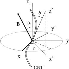
Figure 1: The position of the laboratory coordinate system $x$, $y$ and $z$, the local coordinate $x^{\prime}$, $y^{\prime}$ and $z^{\prime}$ related to CNT flexure and the angles between axes. The direction of a magnetic field B determines the angle $\alpha$.

where $\mu_{B}$ is the Bohr magneton, $\mathbf{S}$ an electron spin, $g_{\perp}=g_{xx}=g_{yy}$ and $g_{\shortparallel}=g_{zz}$ with the principal values of electron $g$-tensor $g_{xx}$, $g_{yy}$, $g_{zz}$. In the presence of flexural thermal vibrations, the system loses the axial symmetry. If the curvature induced by flexural deformation is small (compared to the CNT diameter), one can introduce local Cartesian axes $x^{\prime}$, $y^{\prime}$, $z^{\prime}$ at each point along the CNT (Fig. 1). The angle between the $z$ and $z^{\prime}$ axes is defined as $\theta=\theta(z)$. Then, the Zeeman Hamiltonian in the presence of flexural vibrations can be expressed in the local coordinate system (denoted as $H_{Z}^{\prime}$) by simple substitution $x$, $y$, $z$ $\rightarrow$ $x^{\prime}$, $y^{\prime}$, $z^{\prime}$ in Eq. (1) while retaining the same parameters $g_{\shortparallel}$ and $g_{\perp}$. When one transforms $H_{Z}^{\prime}$ back to the laboratory coordinate $x$, $y$, $z$, the corresponding Hamiltonian $H_{Z}$ shows explicit dependence on the angular displacement. To proceed further we fix the angle $\varphi$ between $x$-axis and $z-z^{\prime}$ plane and take into account the smallness of $\theta$. Keeping the linear terms on $\sin\theta$ , the Hamiltonian can be reduced to the form $H_{Z}=H_{Z}^{(0)}+H_{s-ph}$ with perturbation

$$H_{s-ph}=\Delta g\mu_{B}[(B_{x}S_{z}+B_{z}S_{x})\cos\varphi+(B_{y}S_{z}+B_{z}S_{y})\sin\varphi]\sin\theta,$$ (2)

where $\Delta g=g_{\shortparallel}-g_{\perp}$.

Equation (2) shows that fluctuations of $z^{\prime}$ axis leads to fluctuating effective field that can mediate a spin relaxation. The angular displacements $\theta$ and $\varphi$ are immediate from the transversal deformation $\mathbf{u}$, so that

$$\sin\theta\cos\varphi=\frac{du_{x}}{dz};\hskip 1.4457pt\sin\theta\sin\varphi=\frac{du_{y}}{dz}.$$ (3)

In turn, the $\mathbf{u=u(}z)$ can be expressed in terms of flexural modes. The latter are the two transversal acoustic modes that have orthogonal polarizations $\mathbf{e}_{1}\perp$ $\mathbf{e}_{2}$ (we fix their direction along $x$- and $y$- axes correspondingly) and possess a quadratic dispersion for mode frequency

$$\omega_{\varkappa,q}=\beta q^{2}$$ (4)

with wave number $q$ and polarization $\varkappa=x,y$.Mahan2002 Parameter $\beta$ in Eq. (4) is defined by the diameter $d_{t}$ of CNT and its elastic properties,

$$\beta=\lambda d_{t}v_{t},$$ (5)

where $\lambda=0.56$ (Ref.Mahan2002, ) and $v_{t}=1.4\hskip 1.4457pt10^{6}$ cm/s is a transverse sound velocity.Oshima88 The quadratic dispersion law (4) results in singularity in phonon low energy density of states that impacts the dependencies on magnetic field and temperature as it will be shown below.

If we represent the $\mathbf{u(}z)$ in second quantization form Kittel and substitute it to the Eq. (3) and then to Eq. (2), after some algebra one can find

$$H_{s-ph}=\Delta g\mu_{B}\sum_{\varkappa=x,y}\sum_{q}iqe^{iqz}\sqrt{\frac{\hbar}{2\varrho_{1}A_{0}\omega_{\varkappa,q}}}(B_{z}S_{\varkappa}+B_{\varkappa}S_{z})(a_{\varkappa,q}+a_{\varkappa,-q}^{\dagger}),$$ (6)

where $\varrho_{1}$ is a linear density of CNT with length $A_{0}$, $a_{\varkappa,q}^{\dagger}$ and $a_{\varkappa,q}$ the operators of creation and annihilation of the phonon with wave number $q$ and polarization $\varkappa$.

Hereinafter we use only matrix elements of spin operators that describe the spin-flip transitions between the eigenstates $\left|+\right\rangle$ and $\left|-\right\rangle$ of Hamiltonian $H_{Z}^{(0)}$(1). The diagonal matrix elements can also be responsible for the phase spin relaxation providing the finite phonon lifetime,SK07 we however skip this possibility assuming that phase spin relaxation is conditioned by spin-flip processes.

The symmetry imposes the independence of the problem on azimuth direction angle of a magnetic field. For definiteness sake we fix the $\mathbf{B}$ -direction so that $B_{x}=\sin\alpha$, $B_{y}=0$ and $B_{z}=\cos\alpha$, where $\alpha$ is a vectoral angle between $\mathbf{B}$ and the tube axis $z$ (Fig. 1). Thus diagonalization of $H_{Z}^{(0)}$ gives rise to the $\left|+\right\rangle=\left(\cos\frac{\alpha}{2},\sin\frac{\alpha}{2}\right)$ and $\left|-\right\rangle=\left(-\sin\frac{\alpha}{2},\cos\frac{\alpha}{2}\right)$. Doing so we ignore a small difference in $g_{\shortparallel}$ and $g_{\perp}$. As a result on can find $\left\langle-\left|B_{z}S_{x}+B_{x}S_{z}\right|+\right\rangle=\frac{1}{2}B\cos 2\alpha$ and $\left\langle-\left|B_{z}S_{y}+B_{y}S_{z}\right|+\right\rangle=\frac{i}{2}B\cos\alpha$.

The Eq. (6) is a basic equation that describes the electron spin interaction with flexural modes in CNT. It will be applied for analysis of spin-lattice relaxation in the cases of localized and delocalized electrons in next two sections.

III Spin relaxation of localized electrons

Consider a localized electron in the bias potential applied perpendicular to the semiconductor CNT. Parabolic shape for such potential is a reasonable approximation if we analyze only the ground electronic state.LossDiVincenzo ; KaneNature1998 That assumes quite low temperatures, $k_{B}T\ll\hbar\omega_{0}$, compared with energy space $\hbar\omega_{0}$ to the first excited state. Under these approximations the envelope wave function readsAndo05 $\Psi_{0}=\chi\psi_{T}(\xi)\psi_{L}(\eta)$, where $\xi$ and $\eta$ are the curvilinear coordinates associated with the circumference and longitudinal length of the deflection curve of CNT, $\chi$ is a two-fold amount for $\psi$-function amplitudes at the A and B atoms of a primitive cell. We consider small bends of CNT and join $\eta$ with $z$ axis so that longitudinal part of the $\Psi_{0}$ takes the formSapmaz06

$$\psi_{L}(z)=\sqrt{\frac{2}{\pi d_{0}}}e^{-z^{2}/d_{0}^{2}},$$ (7)

where $2d_{0}=2\sqrt{2\hbar/m^{\ast}\omega_{0}}$ is an extension of the electron localization, $m^{\ast}=2\hbar^{2}/3d_{t}\gamma$ is an effective mass of the semiconducting CNT, $\gamma$ is a transfer matrix element. The implicit forms of the $\chi$ and $\psi_{T}(\xi)$ are irrelevant to the problem under consideration. Besides, we ignore the modifications of the electronic states by the external magnetic field assuming that relevant parameterAndo05 $(d_{t}/2a_{H})^{2}$ is rather small ($a_{H}=\sqrt{c\hbar/eB}$ is the magnetic length).

The averaging of electron-phonon interaction (6) over the $\Psi_{0}$ can be reduced to the calculation of the form-factor $\Phi(q/q_{0})=\left\langle\psi_{L}(z)|e^{iqz}|\psi_{L}(z)\right\rangle$, where $q_{0}\equiv\sqrt{8}/d_{0}$ and

$$\Phi\left(x\right)=e^{-x^{2}}.$$ (8)

Thus, the Hamiltonian of spin-phonon interaction $V_{s-ph}=\left\langle\Psi_{0}|V|\Psi_{0}\right\rangle$ for localized electron can be presented in canonical form

$$H_{s-ph}=\sum_{\varkappa=x,y}\sum_{q}V^{\varkappa,q}(a_{\varkappa,q}+a_{\varkappa,-q}^{\dagger}),$$ (9)

where spin-depended operator is

$$V^{\varkappa,q}=\Delta g\mu_{B}iq\sqrt{\frac{\hbar}{2\varrho_{1}A_{0}\omega_{\varkappa,q}}}\Phi\left(q/q_{0}\right)(B_{z}S_{\varkappa}+B_{\varkappa}S_{z}).$$ (10)

We are looking for the rate of longitudinal spin relaxation $T_{1}^{-1}=w_{+-}+w_{-+}$, which can be evaluated in terms of probability of spin transition $w_{+-}$ ($w_{-+}$) from the spin states $\left|+\right\rangle$ ($\left|-\right\rangle$) to the state $\left|-\right\rangle$ ($\left|+\right\rangle$). In turn, the $w_{+-}$ and $w_{-+}$ can be found by straightforward application of the Fermi golden rule to the Eq. (9). The final result of such calculations takes the form

$$T_{1}^{-1}=\frac{2\pi}{\hbar^{2}}\sum_{\varkappa=x,y}\sum_{q}(2n_{\varkappa,q}+1)\left|V_{+-}^{\varkappa,q}\right|^{2}\delta(\omega_{Z}-\omega_{\varkappa,q}),$$ (11)

where $n_{\varkappa,q}=\left\langle a_{\varkappa,q}^{\dagger}a_{\varkappa,q}\right\rangle=1/\left[\exp(\omega_{\varkappa,q})-1\right]$ is the phonon population factor and $\hbar\omega_{Z}=g\mu_{B}B$ is a Zeeman splitting, a weak anisotropy of g-factor $g$ can be neglected here. The evaluation of the sum in Eq. (11) by means of Eq. (4) with matrix elements of operators in Eq. (10) leads the final result

$$T_{1}^{-1}=\left(\frac{\Delta g}{g}\right)^{2}\frac{\hbar\omega_{Z}^{3/2}}{16\varrho_{1}\beta^{3/2}}\;F(\alpha)\Phi\left(\sqrt{\frac{\omega_{Z}d_{0}^{2}}{4\beta}}\right)\coth\left(\frac{\hbar\omega_{Z}}{2k_{B}T}\right),$$ (12)

where $g\cong g_{\shortparallel},g_{\perp}$, the factor $F(\alpha)$ takes into account the angular dependence of longitudinal relaxation,

$$F(\alpha)=\frac{1}{2}\left(\cos^{2}2\alpha+\cos^{2}\alpha\right).$$ (13)

Equation (13) describes a prominent angular dependence of spin-relaxation rate in CNT. It reaches the maximal value $F(\alpha)=1$ at $\alpha=0$, i.e. a magnetic field applies parallel to the axis of CNT, and reduces this value up to $F(\alpha)=0.22$ at $\alpha=52.5^{\circ}$ (Fig. 2). In the case of perpendicular orientation, $\alpha=90^{\circ}$, only modes with $x$ polarization contribute to relaxation, i.e. $F(\alpha)=0.5$.

IV Spin relaxation of delocalized electrons

Let us consider the spin-flip relaxation for delocalized electrons in semiconductor CNT. This case is most relevant to the spintronic applications, so we extend the consideration up to room temperatures. Assuming small displacements $\mathbf{u}$ we describe the longitudinal component of orbital electronic states in the vicinity of the $K$ valley in terms of plane waves with wave number $k$ counted off from the $K$ point of the Brillouin zone, $\psi_{L}(z)=e^{ikz}/\sqrt{A_{0}}$. This approximation immediately results in momentum conservation when interaction with phonons describes the Hamiltonian (6), i.e. $\left\langle k^{\prime}|e^{iqz}|k\right\rangle=(2\pi/A_{0})\delta(q-k^{\prime}+k)$ and

$$\left\langle k^{\prime}|H_{s-ph}|k\right\rangle=\sum_{\varkappa=x,y}V_{k^{\prime}k}^{\varkappa}(a_{\varkappa,-\Delta k}+a_{\varkappa,\Delta k}^{\dagger}),$$ (14)

where $\Delta k=k^{\prime}-k$, and

$$V_{k^{\prime}k}^{\varkappa}=i\text{sign}(\Delta k)\frac{\Delta g\mu_{B}}{2\pi}\sqrt{\frac{\hbar}{2\varrho_{1}A_{0}\beta}}(B_{z}S_{\varkappa}+B_{\varkappa}S_{z}).$$ (15)

The electron scattering in the vicinity of the $K^{\prime}$ valley gives rise to the same results while intervalley scattering is negligible because it entails the excitation of phonons with giant $q$.

The probability $w_{+-}^{kk^{\prime}}$ of spin-flip $\left|+\right\rangle\rightarrow\left|-\right\rangle$ due to electron scattering $k\rightarrow k^{\prime}$ on the phonons can be found in terms of Fermi golden rule. The averaging over the phonon thermal distribution results in

$$w_{+-}^{kk^{\prime}}=C\left[n_{\Delta k}\delta\left(\Delta E-\hbar\omega_{Z}-\hbar\beta\Delta k^{2}\right)+\left(n_{\Delta k}+1\right)\delta\left(\Delta E-\hbar\omega_{Z}+\hbar\beta\Delta k^{2}\right)\right]$$ (16)

where $C=\pi F(\alpha)(\Delta g\mu_{B}B)^{2}/2\varrho_{1}A_{0}\beta$, $\Delta E=\hbar^{2}(k^{\prime}{}^{2}-k^{2})/2m^{\ast}$. Similarly one can obtain the probability of spin flop $w_{-+}^{kk^{\prime}}$. The net result for electron spin relaxation $\overline{w}_{+-}$ assumes the averaging of the $w_{+-}^{kk^{\prime}}$ over the electron initial state occupation numbers $f_{k}^{+}$ and summation over non-occupied final states $k^{\prime}\left|-\right\rangle$,

$$\overline{w}_{+-}=\sum_{k,k^{\prime}}f_{k}^{+}(1-f_{k^{\prime}}^{-})w_{-+}^{kk^{\prime}}.$$ (17)

The summation over $k$, $k^{\prime}$ has to be replaced by integration in the common fashion. In the case of non-degenerate electrons,

$$f_{k}^{+}=\frac{1}{A_{0}}\sqrt{\frac{2\pi\hbar^{2}}{m^{\ast}k_{B}T}}\exp\left(-\frac{\hbar^{2}k^{2}}{2m^{\ast}}\right).$$ (18)

One can see that the Eqs (16) - (18) are conveniently expressed in terms of new variables $u=k+k^{\prime}$ and $v=k-k^{\prime}$ so that arguments of $\delta$-functions in Eq. (16) transform to the linear form on $u$. The integration over $u$ in Eq. (17) becomes trivial and gives rise to final expression for the spin relaxation rate $T_{1}^{-1}=\overline{w}_{+,-}+\overline{w}_{-,+}$ in the form

$$T_{1}^{-1}=\frac{F(\alpha)}{\sqrt{8\pi}}\left(\frac{\Delta g}{g}\right)^{2}\frac{\sqrt{m^{\ast}(k_{B}T)^{3}}}{\hbar\varrho_{1}\beta}h^{2}\cosh\frac{h}{2}\cosh\frac{\varepsilon h}{2}I(h),$$ (19)

where we introduce the dimensionless parameters $h=\hbar\omega_{Z}/k_{B}T$ and $\varepsilon=2m^{\ast}\beta/\hbar$, and an integral function

$$I(h)=\int_{0}^{\infty}\exp\left(-\frac{1+\varepsilon^{2}}{4\varepsilon}x-h^{2}\frac{\varepsilon}{4x}\right)\frac{dx}{x\sinh(x/2)}.$$ (20)

Taking into account Eq. (5) and definition of $m^{\ast}$, parameter $\varepsilon$ can be estimated as a number $\varepsilon=0.02$ independent on $d_{t}$.

The integrant in Eq. (20) appears as a result of the change of variable $v$ by $x=\hbar\beta v^{2}/k_{B}T$. Asymptotic behavior of the Eq. (20) is $I(h\rightarrow 0)\rightarrow 8/\varepsilon h^{2}$, i.e. the integral diverges at zero magnetic field ($h\rightarrow 0$). Actually this singularity has not physical meaning. If electronic scattering is taking into account, the wave numbers $k$ and $k^{\prime}$ are not longer accurate quantum numbers and $\delta$-functions in the Eq. (16) transform to delta-like functions with finite width and maximum. This limits the value of integrant in Eq. (20) and function $I(h)$ at small $x$ and $h$ correspondingly. Similar situation was discussed in Refs Argyres ; SemenovHFI2007 . Practically, the singularity treatment means that once Zeeman energy $\hbar\omega_{Z}$ becomes of the order of electron energy broadening $\Gamma$, the integral will reach a saturation, i.e. if

$$\hbar\omega_{Z}\lesssim\Gamma,$$ (21)

then $I\left(\hbar\omega_{Z}/k_{B}T\right)\rightarrow I\left(\Gamma/k_{B}T\right)$. As a result, zero magnetic field quenches spin relaxation mechanism under consideration, $T_{1}^{-1}(\omega_{Z}\rightarrow 0)\sim\left(\hbar\omega_{Z}\right)^{2}I\left(\frac{\Gamma}{k_{B}T}\right)\rightarrow 0$. We will not consider this effect in more detail. Fig. 3 presents the function $h^{2}I(h)$ calculated with Eq. (20) without considering the effect of finite $\Gamma$. Note that the $h^{2}I(h)$ exponentially decreases in the limit of large $h$.

V Numerical evaluation and discussion

Equations (12) and (19) define the spin relaxation rate via flexural phonon modes for localized and delocalized electrons. Alternative approach based on the electron spin scattering on disordered nuclei spins $I=\frac{1}{2}$ of ${}^{13}C$ isotopes due to hyperfine interaction was done in the Ref.SemenovHFI2007, . Comparing these mechanisms is performed for chirality vector (8,4) (respectively CNT diameter and effective mass are $d_{t}=0.839$ nm and $m^{\ast}=0.186\hskip 1.4457ptm_{0}$, $m_{0}$ the free electron mass)SemenovHFI2007 with following parameters: $\Delta g=0.005$, $g=2.015$, g-factor $\varrho_{1}=\pi d_{t}\varrho_{2}$ where $\varrho_{2}=9.66\times 10^{-8}$ g/cm² is the mass of graphene sheet per unit area.Ando05 Hereinafter all calculations are performed at $\mathbf{B}$ directed along the tube axis, i.e. $\alpha=0$.

Figure 4 illustrates the temperature and magnetic field dependencies of spin relaxation rate of the electron localized at $2d_{0}=30$ nm. The temperature dependence is typical for one-phonon process of spin-lattice relaxation in semiconductor quantum dot.SK07 At relatively high temperatures ($k_{B}T>\hbar\omega_{Z}$) the population factor for resonant phonons  describes the direct process $T_{1}^{-1}\sim T$ while the temperature independent phonon radiation dominates at $k_{B}T<\hbar\omega_{Z}$. Magnetic field dependence runs from zero through the maximum, which is caused by form-factor at relatively short wavelength of resonant phonon. Dependence on CNT diameter (Fig. 5) stems from the explicit dependencies of form-factor, the $\beta$ [Eq. (5)] and $\rho_{1}$ on $d_{t}$. Both Figs. 4 and 5 display rather long (around few seconds) spin relaxation of localized electrons in CNT at low temperature that makes it attractive for quantum computing application.

The magnetic field and temperature dependencies of spin-relaxation rate calculated with Eq. (19) is shown in Fig. 6 for the delocalized electron (i.e., without taking into consideration the electron scattering effects). Some decreasing attributes to only low temperature relaxation in actual range of the magnetic fields while no significant dependence on ${\mathrm{B}}$ reveals the $T_{1}^{-1}$ starting with $T=40$ K. For the room temperature, Eq. (19) predicts the relaxation time about $T_{1}\simeq 30$ $\mu$s in the wide range of the magnetic fields. The $T_{1}^{-1}$ tends to increase as the temperature goes up while mechanism due to hyperfine interaction possesses the opposite tendency. The increase of the tube diameter suppresses spin relaxation in the case of both mechanisms (Fig. 7). Note that with the exception of very low magnetic field, which corresponds to Eq. (21), the spin relaxation via flexural modes dominates over the processes of electron scattering at nuclei spins. This deduction is based on the comparison of present results and theory developed in Ref. SemenovHFI2007, , where the constant of HFI has been specified, $a_{hf}/2\pi\hbar=-35.8$ MHz. Yazyev

VI Conclusions

A mechanism of electron spin relaxation in carbon nanotubes caused by anisotropy of g-tensor and flexural phonon modes is studied. Relaxation time for localized electron is estimated around a second at low temperature while the spin relaxation of delocalized electrons can reach few tens microseconds at room temperature. As it turned out the proposed mechanism is essentially more efficient than the processes of spin scattering due to hyperfine interaction with isotopes ¹³C. This holds true up to very weak magnetic fields when Zeeman splitting comes up with electron energy broadening. The mechanism reveals specific dependencies on magnetic field orientation (common for both localized and delocalized electrons) and on the magnetic field strength (with perceptible maximum for localized electron and almost flat dependence for delocalized one). Besides, in contrast to processes of scattering on nuclei spins, the temperature augmentation sufficiently increases relaxations rate. These particularities will facilitate the experimental recognition of the mechanism of spin-lattice relaxation in CNT.

Figure 2: Function graph of $F(\alpha)$, which defines the dependence of spin relaxation rate on the angle $\alpha$ between the direction of magnetic field and the axis of CNT for both localized and delocalized electrons.

Figure 3: Plot of function $h^{2}I(h)$, which appears in Eq. (19).

Figure 4: Calculated spin relaxation rates of localized electron in a (8,4) CNT as a function of magnetic field and temperature. Curves 1, 2, and 3 are obtained for $B=1T,$ $0.3T$, and $0.001T$ correspondingly. Curves 4 and 5 are plotted for $T=10$K and $1$K. The size of electron localization is $2d_{0}=30$ nm.

Figure 5: Calculated spin relaxation rates of a localized electron as a function of CNT diameter for different values of magnetic field and temperature and temperatures $T=1$K (left panel)and $T=10$ K (right panel). Curves 1, 2, and 3 correspond to $B=0.001T$, $1T$, and $3T$ respectively. The size of electron localization is $2d_{0}=30$ nm.

Figure 6: Calculated spin relaxation rates for mechanism caused by flexural modes (solid lines) and due to electron scattering on ¹³C isotopes (dashed line) for delocalized electron in a (8,4) CNT as a function of magnetic field at $T=4$K (left panel) and temperature (right panel). The curves 2, 3 and 4 are obtained for $B=0.05$T, $1$T, and $5$T correspondingly. Solid line 1 practically does not change in range of the magnetic field from $B=0.05$T up to $B=5$T.

Figure 7: Calculated spin relaxation rates of delocalized electron as a function of CNT diameter for different values of magnetic field and temperature. Contributions of both HFI (dashed line) and spin-phonon interaction (solid line) are presented for the purpose of comparison. Curves 1, 3, and 6 correspond to $B=0.05$T. Curves 2, 4, and 7 correspond to $B=2$T. Curve 5 does not change in the range of the magnetic field $B=0.05-2$T.

- (1) Carbon Nanotubes: Synthesis, Structure, Properties and Applications, ed. M. S. Dresselhaus, G. Dresselhaus, and P. Avouris (Springer, Berlin, 2000); M. S. Dresselhaus, G. Dresselhaus, and P. S. Eklund, Science of Fullerences and Carnon Nanotubs (Academic, New York. 1996).
- (2) T. Ando, J. Phys. Soc. Japan 74, 777 (2005).
- (3) See, for example, C. Dekker, Phys. Today 52, 22 (1999); T. W. Odom, J. L. Huang, P. Kim, and C. M. Lieber, J. Phys. Chem. B 104, 2794 (2000).
- (4) K. Tsukagoshi, B. W. Alphenaar, and H. Ago, Nature (London) 401, 572 (1999).
- (5) S. Sahoo, T. Kontos, and C. Schönenberger, Appl. Phys. Lett. 86, 112109 (2005).
- (6) H. Mehrez, J. Taylor, H. Guo, J. Wang, and C. Roland, Phys. Rev. Lett. 84, 2682 (2000).
- (7) C.-K. Yang, J. Zhao, and J. P. Lu, Phys. Rev. Lett. 90, 257203 (2003).
- (8) D. Loss and D. P. DiVincenzo, Phys. Rev. A 57, 120 (1998).
- (9) B. E. Kane, Nature (London) 393, 133-137 (1998).
- (10) Y. G. Semenov, K. W. Kim, G. J. Iafrate, Phys. Rev. B 75, 045429 (2007).
- (11) D. V. Bulaev and D. Loss, Phys. Rev. B 71, 205324 (2005).
- (12) G. D. Mahan, Phys. Rev. B 65, 235402 (2002).
- (13) C. Oshima, T. Aizawa, R. Souda, Y. Ishizawa, and Y. Sumiyoshi, Solid State Commun. 65, 1601 (1988).
- (14) C. Kittel, Quantum Theory of Solids (Wiley, New York, 1963).
- (15) Y. G. Semenov and K. W. Kim, Phys. Rev. B 75, 195342 (2007).
- (16) S. Sapmaz, P. J.-Herrero, L. P. Kouvenhoven, and H. S. J. van der Zant, Semicond. Sci. Technol., 21, S52 (2006).
- (17) P. N. Argyres, J. Phys. Chem. Solids 4, 19 (1958).
- (18) O. Chauvet, L. Forro, W. Bacsa, D. Ugarte, B. Doudin, and W. A. de Heer, Phys. Rev. B 52, R6963 (1995).
- (19) O. V. Yazyev, private communication. See also O. V. Yazyev and L. Helm, Phys. Rev. B 72, 245416 (2005).