0710.3162 [hep-th]
String junctions in curved backgrounds,
their stability and
dyon interactions in SYM
Konstadinos Sfetsos and Konstadinos Siampos
Department of Engineering Sciences, University of Patras,
26110 Patras, Greece
sfetsos@upatras.gr,
ksiampos@upatras.gr
Abstract
We provide a systematic construction of string junctions in curved backgrounds which are relevant in computing, within the gauge/gravity correspondence, the interaction energy of heavy dyons, notably of quark-monopole pairs, in strongly coupled SYM theories. To isolate the configurations of physical interest we examine their stability under small fluctuations and prove several general statements. We present all details, in several examples, involving non-extremal and multicenter D3-brane backgrounds as well as the Rindler space. We show that a string junction could be perturbatively stable even in branches that are not energetically the most favorable ones. We present a mechanical analog of this phenomenon.
1 Introduction
String junctions [2, 3] are of particular interest in string theory for several reasons: Due to their BPS nature they can be used to build supersymmetric string networks [4, 5, 6, 7, 8] and they are useful for the description of BPS states in SYM theories [9] and for applications to gauge symmetry enhancement in string theory [10]. The scattering of string modes at string junctions in flat spacetime has been analyzed in [11]. Particularly, important for the purposes in the present paper is the fact that since string junctions connect strings of different type they can be used, within the gauge/gravity correspondence [12], to compute the interaction energy of dyons and in particular of heavy quark-monopole pairs [13].
The purpose of the present paper is to formulate and construct the string junctions appropriate for computing the interaction potentials of heavy dyons at strong coupling, within the gauge/gravity correspondence. This is done for a large class of curved backgrounds away from the conformal point and with reduced or no supersymmetry at all. Having constructed string junction solutions does not imply that the corresponding dyon interaction potentials are physical. One has to at least investigate perturbative stability which will appropriately restrict the parametric space in which the solutions are physically relevant. Such investigations were exhaustively performed [14, 15] for single string solutions useful in computing the heavy quark-antiquark potential. Given these works and in comparison to them we will find that the stability analysis of junctions leads to expected as well as unexpected results, the latter being counterintuitive to stability arguments based on energy considerations.
The organization of this paper is as follows: In section 2 we formulate string junctions in a quite general class of curved backgrounds. We derive general formulae from which the interaction energy of a dyon pair is computed. In section 3 we consider in great detail the stability analysis under small fluctuations of these string junctions aiming at discovering the physically relevant regions. We pay particular attention to the precise formulation of the boundary and the matching conditions at the junction point and derive general statements that isolate the boundaries of stability for all types of perturbative fluctuations. In section 4, we present several examples of string junctions using D3-black branes and multicenter D3-brane solutions which within the AdS/CFT correspondence are relevant for SYM at finite temperature and at generic points in the Coulomb branch of the theory, respectively. In addition, we present the details of string junctions in Rindler space, given its relevance in a variety of black hole backgrounds near the horizon. In section 5, we apply the outcome of the general stability analysis of section 3 to the examples of section 4. We present our conclusions in section 5. In the appendix work out the stability of a classical mechanical system which also exhibits an unexpected perturbative stability similar to the one we found with string junctions.
2 The classical solutions
In this section we develop and present the general setup of the AdS/CFT calculation of the static potential of a heavy static dyon-dyon pair with general NS and RR charges. These computations involve three strings and therefore we will be based to the well-known results for the potential of heavy quark-antiquark pairs of [16] for the conformal case, as extended in [17] for general backgrounds, and to the computation of the interaction energy of a heavy quark-monopole pair in the conformal case [13].
We consider a general diagonal metric of Lorentzian signature of the form
| (2.1) |
Here, denotes the (cyclic) coordinate along which the spatial side of the Wilson loop extends, denotes the radial direction playing the rôle of an energy scale in the dual gauge theory and extending from the UV at down to the IR at some minimum value determined by the geometry, stands for a generic cyclic coordinate, stands for a generic coordinate on which the metric components may depend on and the omitted terms involve coordinates that fall into one of the two latter classes without mixing terms. It is convenient to introduce the functions
| (2.2) |
If the conformal limit can be taken (this is the case in all examples in the present paper except the one involving the Rindler space) we can approximate the metric by that for with radii (in string units) , with being the string coupling. In this limit we have the leading order expressions
| (2.3) |
A string junction consists of three co-planar strings joined at a point as depicted in Fig. 1. The string labelled as 1 has NS and RR charges, the second labelled as 2 has charges, whereas the third straight string labelled by 3 has due to the charge conservation at the junction point. From a microscopic point of view the strings that interact are the fundamental - and -string with charges and , respectively. Any other charge combination should be achievable by performing in this pair an transformation which gives the condition [10]. The first two strings end at the boundary of the space-time at , whereas the straight third string ends at the minimum value of the space-time allowed by the geometry. All three strings meet at the junction point at . Within the framework of the AdS/CFT correspondence, the interaction potential energy of the dyon is given by
| (2.4) |
where
| (2.5) |
is the Nambu–Goto action for a string propagating in the dual supergravity background whose endpoints trace a rectangular contour along one temporal and one space direction, and similar expressions hold for the strings 2 and 3. We will not consider a contribution from the Wess–Zumino terms either because these terms do not exist all or have vanishing contribution within our ansatz for solutions below.
We next fix reparametrization invariance for each string by choosing
| (2.6) |
we assume translational invariance along , and we consider the embedding
| (2.7) |
supplemented by the boundary condition
| (2.8) |
appropriate for a dyon placed at and a dyon placed at . The string with charges extending from the junction point to is straight as is always a solution of the equations of motion (see (2.11) below).
 |
In the ansatz (2.7), the constant value of the non-cyclic coordinate must be consistent with the corresponding equation of motion. This requires that [14]
| (2.9) |
For the ansatz given above, the Nambu–Goto action reads
| (2.10) |
where denotes the temporal extent of the Wilson loop, the prime denotes a derivative with respect to while and are the functions in (2) evaluated at the chosen constant value of . Similar actions are also considered for the string, as well as for the straight string. Independence of the Lagrangian density from implies that the associated momentum is conserved, leading to the equation
| (2.11) |
where are the values of at the turning point for each string, and is the classical solution with the two signs corresponding to the lower (string 1) and upper (string 2). The symbol (not to be confused with the forces in Fig. 1) stands for the function
| (2.12) |
Note that, for the junction point we have that . For the turning points we have that , but they are not necessarily larger than , since the strings 1 and 2 are not actually extending to their turning points. Integrating (2.11), we express the separation length as
| (2.13) |
Finally, inserting the solution for into (2.10) and subtracting the divergent self-energy contribution of disconnected worldsheets, we write the interaction energy of the junction as
| (2.14) |
Ideally, one would like to evaluate the integrals (2.13) and (2) exactly, solve (2.13) for and insert into (2) to obtain an expression for the energy in terms of the separation length and . Then, minimizing this expression with respect to the ’s we will obtain the expression of the in terms of the separation length , which is then identified with the interaction energy of the heavy dyon pair.
However, in practice this cannot be done exactly, except for the conformal case, and Eqs. (2.13) and (2) are to be regarded as parametric equations for and with parameters . A much easier way to find is to impose that the net force at the string junction is zero [3, 5, 11], an approach followed in the present context for the conformal case in [13]. The infinitesimal lengths squared along each string are
| (2.15) |
Hence from the action (2.10) we find that the tensions of the strings at the junction point are and similarly for the other two string that meet at the junction. The angles between the string and the axis at the junction point are computed from
| (2.16) |
where we used (2.11) and took into account that displacements along perpendicular axes are measured by a curved metric. The above explicitly shows that the angles depend on the parameters and . The forces exerted to each of the strings on the plane are
| (2.17) | |||
the first entry being the and the second the component. Demanding that the total force be zero one finds that the angles at the equilibrium point are given by
| (2.18) |
From these expressions the angles are determined in terms of the NS and RR charges of the strings and then from (2.16) one may express in terms of and the string charges. Recalling that is determined by , one ends with the interaction energy being solely a function of and of the strings’ charges as fixed parameters.
We can verify that the approach of fixing the parameters by utilizing the zero force condition at the junction point gives rise to a minimal energy. Since we can not solve (2.13) for in general, we shall recall that we have an implicit expression of in terms of , by inverting (2.13). Since we choose to minimize the energy with respect to , the physical length does not depend on them and we have
| (2.19) |
which can be used together with (2.16) to express the derivative of with respect to as
| (2.20) |
We have not used the no force condition to derive the above in the sense that the angles are not constant except for the equilibrium point. Next, using (2.20) and the zero force condition one can check, after careful algebraic manipulations, that
| (2.21) |
as advertized. Our proof is completely general within our ansatz (2.1) and no-where we did need to explicitly evaluate the various integrals by resorting to specific examples.111 The result is also valid even when in the upper limit of integration infinite is replaced by a finite value, as in the example of the Rindler space below. Had we done so, in the cases where this is possible, we would have ended up with complicated expressions and our proof would have been equivalent to proving certain identities involving, in general, special functions (for instance, for the conformal case see the app. of [13]).
Let us mention that the expression for the interaction energy in terms of length for the configuration of and dyons is invariant under the S–duality transformation , as it should be. However, this is not true for and separately as functions of the auxiliary parameter .
2.1 On the quark-monopole interaction
The most important case arises for the interaction potential of a quark with a monopole with charges and , respectively. In that case it is easily seen from (2) that . It will be useful for later purposes to consider the limit of . In that case the tension of the string corresponding to the monopole becomes very large, so that we expected that it stays almost straight, whereas in order for the forces to balance, the string should hit the straight string almost perpendicularly. This is indeed reflected in the expansions
| (2.22) |
Of course an equivalent expansion exists for , with and interchanged and . In the small string coupling limit we easily infer from (2.16) and (2.22) that the turning points of the strings 1 and 2 are
| (2.23) |
where is the largest root of the equation . In the examples we present in detail below, , except for one case in which it has a smaller value. Therefore the expressions for the separation length (2.13) and the energy (2) for the quark-monopole interaction, become
| (2.24) |
and
| (2.25) |
where we have defined as in (2.12) with replaced by . Thanks to the -duality invariance of the general results (2.13) and (2) identical expressions to (2.24) and (2.25) hold in the large string coupling expansion, where in the correction terms we just replace . Hence, in the limit of small and large string coupling, the energy and the length assume half of their corresponding values for the single string for the quark-antiquary system. We emphasize that this fact does note imply that the spectrum of small fluctuations around the each classical configuration will be the same. Actually we will explicitly demonstrate that the opposite is true, which implies that no matter how stiff two of the strings (the straight and one of the strings 1 or 2) become, its fluctuations do not decouple and affect those of the third string.
3 Stability analysis
We now turn to the stability analysis of these configurations, aiming at isolating in parametric space the physically stable regions and pointing out the similarities and differences with the similar analysis for string configurations dual to the quark-antiquark potential. The small fluctuations about the classical solutions we will discuss, fall into three types: (i) “transverse” fluctuations, referring to cyclic coordinates transverse to the dyon-dyon axis such as , (ii) “longitudinal” fluctuations, referring to the cyclic coordinate along the dyon-dyon axis, and (iii) “angular” fluctuations, referring to the special non-cyclic coordinate . In [14] general results for single string fluctuations of all of the above types for the class of backgrounds with metric (2.1) were derived and used to analyze the stability of heavy quark-antiquark potentials. These are certainly relevant for the investigations of the present paper, so that we review them below, but one has to be careful by paying particular attention to the matching conditions at the junction point of the three strings which affect the parametric space where the stability occurs, in crucial ways.
3.1 Small fluctuations
We parametrize the fluctuations about the equilibrium configuration, by perturbing the embedding according to
| (3.1) |
where the index refers to the three strings forming the junction. Note that we have kept the gauge choice (2.6) unperturbed by using worldsheet reparametrization invariance. We then calculate the Nambu–Goto action for this ansatz and we expand it in powers of the fluctuations. The zeroth-order term gives just the classical action and the first-order vanishes thanks to the classical equations of motion.222A careful treatment of the first-order terms gives rise to boundary terms. Demanding that they vanish turns out to be equivalent to the zero-force condition at the junction point. This can be shown quite straightforward for junctions in a flat spacetime before a gauge choice is made and reproduces the conditions found, for instance, in [11]. However, in curved spaces after the gauge choice is made, one obtains straightforwardly only the -component of the zero-force condition. Switching to the gauge one obtains the -component as well. The resulting expansion for the quadratic fluctuations for the string is written as [14]
where we have used, the condition (2.9) and all functions and their –derivatives are again evaluated at . Writing down the Euler–Lagrange equations for this action, using independence of the various functions from and setting
| (3.3) |
we find that for the strings 1 and 2 the linearized equations for the three types of fluctuations read
| (3.4) | |||
For the straight string the action for the quadratic fluctuations is
| (3.5) | |||||
from which we obtain the equations
| (3.6) | |||
Note that for the straight string the equations can be obtained by formally letting and in (3.4).
Hence determining the stability of the string configurations of interest has been reduced to a eigenvalue problem of the general Sturm–Liouville type
| (3.7) |
where the functions , and are read off from (3.1) and (3.6) and depend parametrically on through the function in (2.12), which in turn is determined by (2.16) in terms of the junction point and the NS and RR charges of the strings. Our aim is to find the range of values of for which is negative. In fact the extremal such value of (the minimum as it turns out) will be decided by determining the zero mode , which is an easier problem. Note also that, although it may seem so, the equations above for the three strings and for given type of fluctuations are not decoupled. The matching conditions at the junction point couple them in an essential manner. This equation can not be solved analytically in general, so that sometimes it is convenient to transform the Sturm–Liouville into a Schrödinger equation and use known approximating analytical methods that boil down to simple numerical problems.
3.2 Boundary and matching conditions
To fully specify our eigenvalue problem, we must impose boundary conditions on the fluctuations at the UV limit , at the IR limit , as well as matching conditions at the junction point at . The boundary condition at the UV are chosen to be
| (3.8) |
where is any of the fluctuations for the strings 1 and 2. These represent the fact that we keep the dyons at fixed points at the boundary. In the far IR at we simply demand, for the string 3 that extends also in there, finiteness of the solution and its -derivative. Otherwise, all perturbations might be driven away from small values.
We demand that the fluctuations as well as their variations in the quadratic actions should be equal at the junction point , so that the latter does not break. Moreover, we demand that the total boundary term resulting in deriving the classical equation of motions from the quadratic actions vanishes. These two requirements give rise to
| (3.9) |
where we have used (2.16) to simplify the second condition.
Identical conditions with those in (3.2) hold for the angular fluctuations as well
| (3.10) |
The appropriate boundary and matching conditions for the fluctuations should be found first in a coordinate system in which the classical solution does not change. This is simply given by [14]
| (3.11) |
and is easily checked that the classical solution is not perturbed at all. This redefinition does not affect the - and –fluctuations since they have trivial classical support and we keep only linear, in fluctuations, terms. At the junction point the fluctuations are continuous and this leads to a discontinuity for the fluctuations due to (3.11) for the strings 1 and 2. As before, we demand that the total boundary term resulting in deriving the classical equation of motions from the quadratic actions vanishes, keeping in mind that the variations of the ’s in their quadratic actions should be equal at the junction point. With the use of (2.16) we have the following conditions for the fluctuations
| (3.12) |
3.3 Zero modes
As we have noted we can obtain the boundary of stability in parametric space by studying the zero-mode problem. Hence, we examine closely the three distinct types of fluctuations.
3.3.1 Transverse zero modes
For the transverse fluctuations the zero mode solution obeying (3.8) for the strings 1 and 2 is
| (3.13) |
where the ’s are multiplicative constants. The zero mode solution for the straight string is
| (3.14) |
When we specialize this expression in our examples we will see that either and/or diverges when , so we choose in order for the solution and its derivative to remain finite. Thus and the zero mode solution becomes irrelevant for the stability analysis. From (3.2) and the zero force condition, one finds a linear homogeneous system of algebraic equations for and , whose determinant should vanish for non-zero solutions to exist. In this way we find the following condition
| (3.15) |
Since this condition cannot be satisfied and therefore the transverse zero modes do not exist, rendering the corresponding fluctuating modes as stable. Our finding is similar to the conclusion that the transverse fluctuations of the single string fluctuation corresponding to the potential of heavy quark-antiquark pairs are also stable [14].
3.3.2 Longitudinal zero modes
We next turn to the longitudinal fluctuations. The zero mode solution obeying (3.8) for the strings 1 and 2 is
| (3.16) |
where the ’s are multiplicative constants. The zero mode solution for the straight string is
| (3.17) |
As before, when we specialize this expression in our examples we will see that either and/or diverges when , so we choose in order for the solution and its derivative to remain finite. Therefore the zero mode fluctuation becomes irrelevant for the stability analysis. Similarly to before, from (3.12) and the zero force condition one finds the following relation
| (3.18) |
This is an equation for in terms of the string coupling and the strings’ charges, which can be solved numerically. We will denote its solution, whenever it exists, by . In general we will have expansions of the form
| (3.19) |
In the most important case of a quark-monopole interaction, -duality invariance of the result dictates that and therefore the two perturbative expansions above contain the same information. Namely, and all coefficients are equal, i.e. . Actually, then the critical value does not change significantly from its leading order values , the reason being that the small and large results actually coincide and therefore there is not much room for big changes in between. We show below that the leading term can be computed by (3.24) which is an approximative version of (3.18). In the examples below the leading order result for from (3.24) and that computed for using (3.18) differ by two to ten percent.
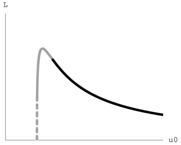
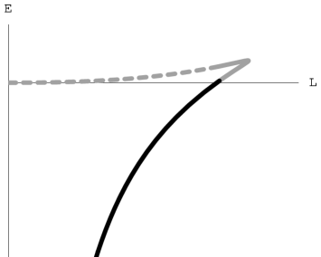
A natural question is whether or not the value of coincides with that corresponding to the maximum value of , labelled by if that exists, below which the energetically less favorable branch in the diagram starts (a typical case is presented in fig. 2).
 |
 |
| (a) | (b) |
This might have been expected since in [14, 15] it was shown quite generally that an instability of longitudinal fluctuations of a single string used to compute the heavy quark-antiquark potential, occurs precisely at the solutions of the equation (which is identical to ). In our case following similar manipulations as in [14] and using (2.16) at the equilibrium point where the ’s are constant, in order to find the derivatives of with respect to , we obtain
| (3.20) |
which are indeed proportional to each other and where we have defined333In cases, such as in Rindler space, where the upper limit of integration is finite, i.e. , then there appears an additional term in the expressions below given by computed at and also we replace infinity by in the upper limit of integration.
| (3.21) |
The value of for which (3.18) is satisfied is different from for which . In fact, in the examples we will explicitly work out, it occurs at smaller values, which implies that part of the upper branch of the solution is still perturbatively stable although energetically not favorable. However, the disconnected configuration becomes energetically favorable for all positive values of the energy. Thus part of the upper branch which is perturbatively stable is in fact metastable. The fact that can be demonstrated quite generally in the small coupling constant limit for the most significant case, namely for the quark-monopole system. We may show that
| (3.22) |
with an analogous expression for . From this we compute the leading term in an expansion of the values for which the maximum energy and length occur analogous to (3.19). Using (2.22), (2.23) and the general identity
| (3.23) |
proved by partial integration, we may show that the zero-mode condition (3.18) becomes
| (3.24) |
from which one computes the leading order value of in the expansion (3.19), namely . Coming from different conditions we have that generically and this explicitly demonstrates that the value for found by requiring maximum length and energy is different than the value of found by requiring the existence of a zero mode for the longitudinal fluctuations which signals perturbative instability of the system.
We note that the condition (3.24) can be directly obtained from the boundary conditions (3.12) specialized to the zero mode solution for the longitudinal fluctuations. In the derivation one should be careful and absorb a factor of into the overall amplitude of the string 2. In this way it becomes apparent that although in the small coupling limit the string 2 becomes stiff and approximately straight, its ultra small in strength fluctuations couple to those of the string 1. Similar considerations can be given for the higher modes as well. The above comments explain also why although in the limit (or ) the turning point (or ) and therefore the corresponding equation for the fluctuations (3.4) becomes the same as the equation that appears in the case of the single string for the quark-antiquark system [14], the conditions for the existence of the zero mode are different in the two cases. They are so due to the different boundary conditions.
Finally, we comment on whether or not the heavy dyon-dyon potentials as computed within supergravity using the AdS/CFT correspondence violate some general principles regarding the strength and sign of the corresponding force. For instance, for the quark-antiquark potential it turns out that the force should always be attractive with strength an ever non-increasing function of the separation distance [18]. This is a concavity condition for the quark-antiquark potential and implies that the upper branch in the plot should be disregarded, in full agreement with the results of [14, 15] employing perturbative stability. In our case, using (3.3.2), we can show that
| (3.25) |
which can be written in a symmetric way under an exchange of the strings 1 and 2 using the -component of the non-force condition. The expressions (3.25) for the dyon-dyon potential are analogous to those found in [17] for the quark-antiquark potential. Hence, the force is always attractive, but for the upper branch in the plot in which , has an increasing strength. On the other hand we have found that part of the upper branch is perturbatively stable, so that requiring concavity seems to be a stricter condition than perturbative stability. However, concavity is not a condition that gauge theory analysis of Wilson loops for heavy quark-monopole pairs requires. One can derive using reflection-positivity, that the energy of this pair is larger or equal than the average of the energies of the quark-antiquark and monopole-antimonopole systems.444We thank C. Bachas for providing this information. This condition is rather trivially satisfied in our case, provided we use the physical lower branches of the two pairs.
3.3.3 Angular zero modes
For the angular zero modes we cannot explicitly write down the solution for the zero mode due to the presence of the restoring force term in the corresponding Sturm–Liouville equation in the third lines of (3.1) and (3.6). Therefore, in this case we have to work out explicitly the result in the various examples we will present. As it was shown in previous work [14, 15] one can use approximate analytic methods in which the Schrödinger description of the differential equation (3.7) plays an important role.
4 Examples of classical string junction solutions
In this section, we study first the behavior of the dyon-dyon potentials emerging in Wilson-loop calculations for non-extremal and multicenter D3-brane backgrounds. Since we will work with the Nambu–Goto action, we need mention in the expressions below only the metric and not the self-dual five-form which is the only other non-trivial field present in our backgrounds. At the end we work out the example of the Rindler space which captures the behavior of black holes in various dimensions near the horizon.
4.1 Non-extremal D3-branes
We start by considering a background describing a stack of non-extremal D3-branes [19]. In the field-theory limit the metric reads
| (4.1) |
where the horizon is located at and the corresponding Hawking temperature is . This metric is just the direct product of –Schwarzschild with and it is dual to SYM at finite temperature. For the calculations that follow, it is convenient to switch to dimensionless variables by rescaling all quantities using the parameter . Setting and and introducing dimensionless length and energy parameters by
| (4.2) |
we see that all dependence on drops out so that we may set in what follows. The functions in (2) depend only on (reflecting the fact that all values of are equivalent) and are given by
| (4.3) |
In this case , coinciding with the location of the horizon. For the dyon-dyon potential we find that the separation length is given in terms of the junction point as
| (4.4) |
whereas the energy is given by
In the above is the Appell hypergeometric function and . From (2.16) one finds that the turning points of the two strings are given by
| (4.6) |
where the angles are given by (2), in terms of the strings’ charges. From (3.3.2) we have in this case
| (4.7) |
The function has a single global maximum for any value of the string coupling. Its location depends on the string coupling and we obtain the following expansion for the quark-monopole system
| (4.8) |
For , only the disconnected solution exists. For , Eq. (4.1) has two solutions for , corresponding to a short and a long string and, accordingly, is a double-valued function of . The behavior described above is shown in the plots of Fig. 2 and we see that it is very similar to the behavior of the and for the heavy quark-antiquark system [20]. However, as we have pointed out and we will see later in detail the upper branch, although energetically less favorable than the lower one, it is not unstable in its entirety. We note that the classical string junction in this case has also been examined in [21] where the behavior of fig. 2 was also noted.
4.2 Multicenter D3-branes on a sphere
We now proceed to the case of multicenter D3-brane distributions. These distributions [22, 23] constricted as extremal limit of rotating D3-brane solutions [24, 25] have been used in several studies for the Coulomb branch of SYM within the AdS/CFT correspondence, starting with the works of [17, 26]. Here, we will concentrate on the particularly interesting cases of uniform distributions of D3-branes on a three-sphere.
The field-theory limit of the metric for D3-branes uniformly distributed over a 3-sphere with radii reads
| (4.9) | |||||
where
| (4.10) |
It is convenient to switch to dimensionless variables by rescaling all quantities using the parameter . Setting and and introducing dimensionless length and energy parameters by
| (4.11) |
we see that all dependence on drops out so that we may set in what follows., we write the functions in (2) as
| (4.12) | |||
Therefore the conditions (2.9) are satisfied only for and . We examine these two cases in turn.
4.2.1 The trajectory corresponding to
In this case and the integrals for the dimensionless length and energy read
| (4.13) | |||||
and
where and are the incomplete elliptic integrals of the first, second and third kind respectively, while and are the corresponding complete ones and
| (4.15) |
From (2.16) one finds that
| (4.16) |
where the angles are given by (2). The function has a single global maximum depending on the string coupling . The situation is similar to the quark-antiquark potential in this background [17] and to the case of string junctions on black -branes in the present paper. The general behavior is shown in the plots of Fig. 2.
4.2.2 The trajectory corresponding to
In this case , but and the integrals for the dimensionless length and energy read
| (4.17) | |||||
and
where now
| (4.19) |
 |
 |
| (a) | (b) |
From (2.16) one finds that
| (4.20) |
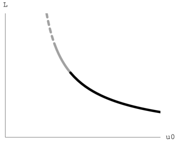
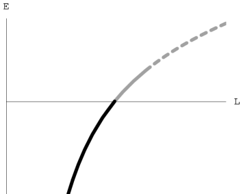
where angles are given by (2). In this case is a monotonously decreasing function which approaches infinity as and zero as and hence no maximal length exists, Eq. (4.17) has a single solution for given the length and consequently is a single-valued function of . This behavior is shown in Fig. 3. This confining behavior is similar to what was found for the quark-antiquark system in [17].
4.3 Rindler Space
Our next example is based on the Rindler space, which it is a portion of flat Minkowski space. In this space an observer experiences the Unruh effect, perceiving the inertial vacuum as a state populated by a thermal distribution of particles at a temperature , where is the surface gravity. Black hole solutions near the horizon behave like the Rindler space, so that the study of string in this background serves more general purposes. In [27, 15] the string configuration corresponding to an open string with its two endpoints located at the same radius (instead of ) we studied. Moreover, we have proven that this problem is exactly equivalent to the classical-mechanical problem of the shape of a soap film suspended between two circular rings and we have also performed a small fluctuations analysis around this classical configuration.
The metric for Rindler space has the form
| (4.21) |
where is the radial direction with the Rindler horizon corresponding to and is a generic spatial direction. It is natural to extend the computation of [15] to the case of sting junctions with the end points of strings 1 and 2 at and the third straight string stretching to . For convenience we pass to dimensionless units
| (4.22) |
and then we use the formalism of section 2 which readily applies to this setup. The length and the energy of the string are determined by Eqs. (2.13) and (2) (without the subtraction term for the energy and the upper limit in the integration changed to 1) which for our case read
| (4.23) |
and
| (4.24) | |||||
From (2.16) one finds that
| (4.25) |
where the angles are given by (2). The function has a single global maximum. Its location, depends on the string coupling . For small values of the latter we get the expansion
| (4.26) |
The situation is similar to that depicted in the plots of fig. 2.
5 Examples of stability analysis
In this section we apply the stability analysis developed in section 3 to the string solutions reviewed in section 4. We find that for the non-extremal D3-brane, the sphere with and the Rindler space we have a longitudinal instability corresponding to the upper branch of the energy curve, for the sphere with we have angular instabilities towards the IR, even though the potential has a single branch.
5.1 The conformal case
For completeness we consider first the conformal case, corresponding to the or limit of any of the above solutions. The classical string junction solution has been constructed in [13]. Since there is no -dependence, the fluctuations are equivalent to the transverse -fluctuations and therefore stable. On the other hand for the longitudinal fluctuations we have to solve (3.18). From (2.16) one finds that
| (5.1) |
where the angles are given by (2). Moreover we compute
| (5.2) |
Using the above, we may check that (3.18) has no solution for any value of string coupling , thus we verify that indeed string junctions are stable in the conformal case.
5.2 Non-extremal D3-branes
We proceed next to the case of non-extremal D3-branes, where we recall that the potential energy is a double-valued function of the separation length. As before, since there is no -dependence, the fluctuations are equivalent to the -fluctuations and stable. For the longitudinal fluctuations we have to solve (3.18), where
| (5.3) |
Equation (3.18) has a solution for any value of string coupling . This value , is smaller than the value in which the maximum of the length occurs. In the limit of small coupling constant for the quark-monopole system we have shown that we can approximate (3.18) by the condition (3.24) which in our case becomes
| (5.4) |
Its solution gives the leading order result for the critical value in which instability occurs
| (5.5) |
where we have included the first correction as well. This expansion is different than the expansion of in (4.8). Thus the whole upper branch is not entirely unstable, a behavior not expected from energetic considerations. Let’s compare the maximum length of the screened interaction for the cases of the quark-antiquark and the quark-monopole interactions. As varies from small to large values the maximum length is , whereas for the quark-antiquark pair . We see that the quark-monopole pair is screened twice as strong as the quark-antiquark pair. This is a general feature in all of the examples we encounter in this paper.
5.3 Multicenter D3-branes on a sphere
The results of the stability analysis for the two orientations for the sphere distribution are presented below.
5.3.1 The trajectory corresponding to
Angular fluctuations are stable due to the fact that, as in [14], we may transform, for each string separately, the problem into a Schrödinger equation with a positive potential for all values of . For the longitudinal fluctuations we have to solve (3.18), where
| (5.6) |
This has a solution for all values of the string coupling. In the limit of small string coupling for the quark-monopole system the condition (3.24) reads explicitly
| (5.7) |
giving the leading order result for the critical value in which instability occurs
| (5.8) |
Thus, part of the upper branch of the solution is perturbatively stable as in the case of the string junction based on the non-extremal D3-brane solution. As before, we compare the maximum length of the screened interaction for the cases of the quark-antiquark and the quark-monopole interactions. As varies from small to large values the maximum length in the quark-monopole interaction is , whereas for the quark-antiquark pair .
5.3.2 The trajectory corresponding to
Longitudinal fluctuations are stable since an explicit check of (3.18) shows that it has no solution for any value of string coupling . Alternatively, we may transform the problem into a Schrödinger problem as in [14] with an everywhere positive potential. For the angular fluctuations the potential is just constant
| (5.9) |
The change of variables for the two string is
| (5.10) |
where and are given by
| (5.11) |
The zero mode of the Schrödinger equation for the strings read
| (5.12) |
where are multiplicative constants. The straight string 3 plays a rôle in the boundary conditions, the reason being that the mass term is present in the equation for the angular fluctuations even for the zero mode. For the straight string we have two linear independent solutions and , where the appropriate change of variable is
| (5.13) |
We examine in detail the case where only is used and comment on the general linear combination later. From the matching conditions in (3.2) one finds the following condition
| (5.14) |
For the quark-monopole case we may use that , to simplify it a bit. Furthermore, in the small string coupling limit (5.14), becomes
| (5.15) |
which is a more explicit and easy to handle transcendental equation. Hence, the solution for the leading order critical values for which instability of the angular perturbations occur is
| (5.16) |
The confining behavior turns out to be unstable since (5.14) has a solution for any value of the string coupling . As varies from small to large values, the maximum length of the quark-monopole interaction is , whereas for the quark-antiquark pair .
Let’ s mention that, had we used the general solution of the Scrödinger equation, that is , we would have obtained similar results for any phase with the exception of for which case no instability occurs. Hence the above considerations and results are quite generic.
Finally let’s note that, in order keep the discussion at a reasonable length, we refrained from explicitly presenting the details for the other important uniform distribution of D3-branes, namely, that on a disc. We mention the end result: For the solution is stable against all types of small fluctuations, while for it is stable against longitudinal fluctuations and unstable against angular ones after a certain separation length. This behavior reveals the expected screening behavior which moreover is practically independent of the orientation of the string and similar to that for the case of the quark-antiquark potential studied in full detail in [14].
5.4 Rindler Space
Finally, we consider the case of the Rindler space. Fluctuations of the single string solution corresponding to the heavy quark-antiquark potential have been considered in [15, 27]. Turning to our case, we see from the form of the metric only the longitudinal fluctuations are relevant for our discussion, so that we have to solve (3.18), where
| (5.17) |
Equation (3.18) has a solution for all values of the string coupling and we have the same behavior as in fluctuations in the non–extremal D3–branes. For small values of the string coupling latter we get the expansion
| (5.18) |
We see that it is different from the expansion of in (4.26) corresponding to the maximum of the length and the energy. Hence, the behavior is similar to that represented in fig. 3.
6 Discussion
In this paper we have constructed string junctions on general backgrounds and used them to compute the interaction energy of heavy dyons at strong coupling within the AdS/CFT correspondence. The most important case is that of the quark-monopole pair for which we paid particular attention. Then we turned into the perturbative stability analysis of these solutions which is important to distinguish the physically relevant regions in which the potentials can be trusted. We formulated and further investigated general conditions for the existence of instabilities. Starting with the conformal case we indeed verified that there are no instabilities at the conformal point of SYM, as expected. Nevertheless, we emphasize here that in the -deformed conformal solution of [28], as well as for all backgrounds that asymptote this, there is an instability for certain angular fluctuations. The reason is identical to the case of a single string for the quark-antiquark potential that was found in [15] (see section 4.3.1) and occurs for values of the real deformation parameter (in the standard notation) larger than a certain critical value (we remark that the classical string junction of the -deformed background of the disc D3-brane distribution has been considered in [29] and should suffer from this instability).
We found that part of the branches of the potential energy versus length that could be disregarded on energetic considerations can be perturbatively stable. The reason is traced to the fact that the matching conditions at the junction point allow for interaction of all strings in the junction that enhances its stability. This is unlike the findings in [14, 15] for the quark-antiquark potential according to which the perturbative instability renders energetically unfavorable branches as unstable. We pointed out that this result is not in conflict with general considerations on the quark-monopole potential. For instance, there is no concavity condition as is in the case of the quark-antiquark potential. We found that the confining behavior of the dyon-potential in the Coulomb branch of the SYM with vacuum expectation values distributed uniformly on a sphere, is unstable. This is similar to the result of [14] for the seemingly confining behavior of the quark-antiquark potential for the same distribution. It is quite remarkable that demanding perturbative stability of the string configurations renders as physically unacceptable the confining behavior, which indeed is not expected from gauge theory considerations.
Our general formalism was based on a diagonal class of metrics (2.1). It can be extended to supergravity backgrounds in which off-diagonal metric elements appear and in which additional background form fields couple in the Wess–Zumino part of the string actions in the junction, in analogy with [15] for the quark-antiquark case. In particular, this will cover, within the AdS/CFT correspondence, interactions of moving dyons in hot quark-gluon plasmas. We expect that also in this case the associated energy will have two branches with the upper one being only partly unstable. The behavior found in [30], namely that the maximum length behaves for high enough velocity as is expected to persists with the overall numerical coefficient replaced by, roughly, its half.
It will be interested to extend our analysis to junctions involving more than three strings where we believe similar phenomena with the triple-junctions considered here will be found. A more interesting generalization is to consider systems of multiple external particles at finite temperature and examine to what extend they prefer, under small perturbations to split, with raising temperature, into smaller systems. This possibility was argued for, based on energy considerations, in [31] who examined in detail the interaction energy for the system of a quark, a monopole and a dyon.
Finally, it has been proposed that - and -superstrings could have been produced at the early Universe, then expanded at a cosmic size and that their network properties by forming junctions make them distinguishable [32] from gauge theory cosmic strings (see, for instance, [33]). The no-force condition for a stationary junction to form, gives rise to a locally flat space time [34], much-like the case of single cosmic strings [35]. Small fluctuations of cosmic string junctions on flat spacetime have been analyzed [36] in closed analogy with corresponding work on superstring junctions (see, for instance, [33]). In view of the above remarks it will be very interested to study the formation and stability of cosmic size string junctions in cosmological backgrounds, by adapting the results and techniques of the present paper, to such cases.
Acknowledgments
We would like to thank S. Avramis for useful discussions. We acknowledge support provided through the European Community’s program “Constituents, Fundamental Forces and Symmetries of the Universe” with contract MRTN-CT-2004-005104, the INTAS contract 03-51-6346 “Strings, branes and higher-spin gauge fields”, the Greek Ministry of Education programs with contract 89194. In addition, K. Siampos acknowledges support provided by the Greek State Scholarship Foundation (IKY).
Appendix A An analog from classical mechanics
Longitudinal string fluctuations exhibit a behavior which is not expected from the energetics of the configurations. However, this behavior can be found in the classical mechanics problem of determining the shape of a thin soap film stretched between two rings appropriately, modified to serve our purposes. We briefly review first the solution of the unmodified classical problem which is a catenary and can be found in standard textbooks [37]. In the notation of the present paper and of the appendix of [14] the cylindrically symmetric solution reads
| (A.1) |
in terms of the integration constant parameter . The potential energy and length of the soap film are given by the following expressions
| (A.2) |
Hence, is a double-valued function of with the energetically favorable branch having lower energy for a given distance, corresponding to a shallow catenary, whereas the upper branch corresponds to a deep catenary. There is also the Goldschmidt solution, with two disconnected soaps in the two rings with energy . Thus we have the same qualitative behavior as in the classical solution of the non–extremal D3–branes, depicted in fig. 2. The value of at the turning point is leading to the maximal length of . The Goldschmidt solution becomes energetically favorable at a higher value of , corresponding to a smaller value of . The perturbative small fluctuation analysis has been performed in [38] and in [14]. The small fluctuations stability analysis of this solution gives the expected result that the upper, energetically unfavorable, branch is perturbatively unstable.
We would like to add an extra term to the quadratic fluctuations (see Eq.(A-1) in appendix A of [14]) that, to leading order, would not affect the energy of the solutions and then check whether part of the upper branch becomes perturbatively stable due to this modification of the action. In order to fulfill the above requirement imagine that we first let the soap film assume its shape given by (A.1) and then we turn on the perturbation which we take it to be quadratic in the normal fluctuations of the soap film surface. The normal fluctuations decouple from the two tangential perturbations which moreover are trivial [14]. This will not affect the classical solution and its energy, but will certainly modify the stability analysis. There are several such terms that we may add. Here we choose to present the two most natural ones.
In the first we add a term to the potential that acts only at the minimum of the catenary at
| (A.3) |
where the factor is introduced for convenience. For the normal perturbations, we define , we separate variables according to
| (A.4) |
and eventually we end up with the Sturm– Liouville equation
| (A.5) |
subject to the following boundary conditions
| (A.6) |
representing fixed endpoints. Equation (A.5) can not be easily solved for non-vanishing values of , but we can obtain useful information for our stability problem by considering the zero–mode problem having . The transformation turns (A.5) to an associated Legendre equation with the general solution given by a linear combination of (they vanish identically unless ) and , with different coefficients to the regions left and right of . However, we know from the work in [14] that in the absence of the extra term (for ), only for a zero mode exists for the value we mentioned above. Since the modification is by an repulsive -function term the possibility of having zero mode solutions in the presence of it for , is definitely excluded. Hence we concentrate to the case with . The continuity of the solution at , the discontinuity of its derivative, as read off from (A.5), and the boundary conditions (A.6), give a linear homogeneous system for the four independent coefficients which in order to have non-trivial solution should have a vanishing determinant resulting to the condition
| (A.7) |
This equation has a solution for all , which varies monotonously from to 0, as . Importantly, the product and therefore the term (A.3) we have added, remain finite. For small and large values of we have the behaviors
| (A.8) |
and
| (A.9) |
An alternative to (A.3) potential term is
| (A.10) |
where the factor is, as before, introduced for convenience. In the Sturm–Liouville equation (A.5) we replace . The same transformation gives an associated Legendre equation with the general solution given by a linear combination of and , where . For identical reasons as before we concentrate to the case with and in fact refining the argument we should have that in order to find a normalizable zero mode. Imposing the boundary condition (A.6) and demanding that the determinant of the resulting linear homogeneous system for two independent coefficients has non-trivial solutions, we obtain the condition
| (A.11) |
This can only be solved numerically and as before the product remains finite. For small and large values of we have the behaviors
| (A.12) |
and
| (A.13) |
In both of the above examples we see that the critical value can get arbitrarily small, which implies that the entire upper, energetically less favorable branch corresponding to the deep catenary, can become perturbatively stable.
References
- [1]
- [2] O. Aharony, J. Sonnenschein and S. Yankielowicz, Nucl. Phys. B474 (1996) 309, hep-th/9603009.
- [3] J.H. Schwarz, Nucl. Phys. Proc. Suppl. 55B (1997) 1, hep-th/9607201.
- [4] K. Dasgupta and S. Mukhi, Phys. Lett. B423 (1998) 261, hep-th/9711094.
- [5] A. Sen, JHEP 9803 (1998) 005, hep-th/9711130].
- [6] S.J. Rey and J.T. Yee, Nucl. Phys. B526 (1998) 229, hep-th/9711202.
- [7] M. Krogh and S. Lee, Nucl. Phys. B516 (1998) 241, hep-th/9712050.
- [8] Y. Matsuo and K. Okuyama, Phys. Lett. B426 (1998) 294, hep-th/9712070.
- [9] O. Bergman, Nucl. Phys. B525 (1998) 104, hep-th/9712211.
- [10] M.R. Gaberdiel and B. Zwiebach, Nucl. Phys. B518 (1998) 151, hep-th/9709013.
- [11] C.G. Callan and L. Thorlacius, Nucl. Phys. B534 (1998) 121, hep-th/9803097.
- [12] J.M. Maldacena, Adv. Theor. Math. Phys. 2 (1998) 231, Int. J. Theor. Phys. 38 (1999) 1113, hep-th/9711200. S.S. Gubser, I.R. Klebanov and A.M. Polyakov, Phys. Lett. B428 (1998) 105, hep-th/9802109. E. Witten, Adv. Theor. Math. Phys. 2 (1998) 253, hep-th/9802150 and Adv. Theor. Math. Phys. 2 (1998) 505, hep-th/9803131.
- [13] J.A. Minahan, Adv. Theor. Math. Phys. 2 (1998) 559, hep-th/9803111.
- [14] S.D. Avramis, K. Sfetsos and K. Siampos, Nucl. Phys. B769 (2007) 44, hep-th/0612139.
- [15] S.D. Avramis, K. Sfetsos and K. Siampos, Nucl. Phys. B793 (2008) 1, arXiv:0706.2655 [hep-th].
- [16] J.M. Maldacena, Phys. Rev. Lett. 80 (1998) 4859, hep-th/9803002. S.J. Rey and J.T. Yee, Eur. Phys. J. C22 (2001) 379, hep-th/9803001.
- [17] A. Brandhuber and K. Sfetsos, Adv. Theor. Math. Phys. 3 (1999) 851, hep-th/9906201.
- [18] B. Baumgartner, H. Grosse and A. Martin, Nucl. Phys. B254 (1985) 528. C. Bachas, Phys. Rev. D33 (1986) 2723.
- [19] G.T. Horowitz and A. Strominger, Nucl. Phys. B360 (1991) 197.
- [20] S.J. Rey, S. Theisen and J.T. Yee, Nucl. Phys. B527 (1998) 171, hep-th/9803135. A. Brandhuber, N. Itzhaki, J. Sonnenschein and S. Yankielowicz, Phys. Lett. B434 (1998) 36, hep-th/9803137 and JHEP 9806 (1998) 001, hep-th/9803263.
- [21] D.K. Park, Nucl. Phys. B618 (2001) 157, hep-th/0105039.
- [22] P. Kraus, F. Larsen and S.P. Trivedi, JHEP 9903 (1999) 003, hep-th/9811120.
- [23] K. Sfetsos, JHEP 9901 (1999) 015, hep-th/9811167.
- [24] M. Cvetic and D. Youm, Nucl. Phys. B477 (1996) 449, hep-th/9605051.
- [25] J.G. Russo and K. Sfetsos, Adv. Theor. Math. Phys. 3 (1999) 131, hep-th/9901056.
- [26] D.Z. Freedman, S.S. Gubser, K. Pilch and N.P. Warner, JHEP 0007 (2000) 038, hep-th/9906194.
- [27] D. Berenstein and H.J. Chung, Aspects of open strings in Rindler Space, arXiv:0705.3110 [hep-th].
- [28] O. Lunin and J.M. Maldacena, JHEP 0505 (2005) 033, hep-th/0502086.
- [29] C. Ahn, Phys. Lett. B641 (2006) 481, hep-th/0605012.
- [30] H. Liu, K. Rajagopal and U.A. Wiedemann, Phys. Rev. Lett. 98 (2007) 182301, hep-ph/0607062, hep-ph/0607062.
- [31] U.H. Danielsson and A.P. Polychronakos, Phys. Lett. B434 (1998) 294, hep-th/9804141.
- [32] J. Polchinski, AIP Conf. Proc. 743 (2005) 331 [Int. J. Mod. Phys. A20 (2005) 3413] [arXiv:hep-th/0410082]. E.J. Copeland, R.C. Myers and J. Polchinski, JHEP 0406 (2004) 013, hep-th/0312067.
- [33] A. Vilenkin and E. Shellard, Cosmic strings and other gravitational defects, Cambridge University Press, 1994. M.B. Hindmarsh and T.W. B. Kibble, Rept. Prog. Phys. 58 (1995) 477, hep-ph/9411342.
- [34] R. Brandenberger, H. Firouzjahi and J. Karouby, Lensing and CMB Anisotropies by Cosmic Strings at a Junction, arXiv:0710.1636 [hep-th].
- [35] A. Vilenkin, Phys. Rev. D23 (1981) 852.
- [36] E.J. Copeland, T.W. B. Kibble and D.A. Steer, Phys. Rev. Lett. 97 (2006) 021602, hep-th/0601153 and Phys. Rev. D75 (2007) 065024, hep-th/0611243.
- [37] C. Caratheodory, Calculus of Variations and Partial Differential Equations of the First Order, American Mathematical Society, 1999. G.A. Bliss, Calculus of Variations, Chicago, IL: Open Court, 1925. R. Courant and H. Robbins, What is Mathematics?, Oxford University Press, Oxford, 1941. G.B. Arfken and H.J. Weber, Mathematical Methods for Physicists, 6th edition, 2005, Elsevier Academic Press.
- [38] L. Durand, Am. J. Phys. 49 (1981) 334.