The twist-3 parton distribution function $e^{a}(x)$ in large-$N_{c}$ chiral theory

Abstract

The chirally-odd twist-3 parton distribution function $e^{a}(x)$ of the nucleon is studied in the large-$N_{c}$ limit in the framework of the chiral quark-soliton model. It is demonstrated that in spite of properties not shared by other distribution functions, namely the appearance of a $\delta(x)$-singularity and quadratic divergences in $e^{a}(x)$, an equally reliable calculation is possible. Among the most remarkable results obtained in this work is the fact that the coefficient of the $\delta(x)$-singularity can be computed exactly in this model, avoiding involved numerics. Our results complete existing studies in literature.

I Introduction

The twist-3 parton distribution function $e^{a}(x)$ Jaffe:1991ra was so far subject to modest interest in literature, in spite of its remarkable theoretical properties, because of its chirally odd nature which makes it difficult to access in experiment. The probably most striking theoretical property is the existence of a $\delta$-function-type singularity at $x=0$ in $e^{a}(x)$ which follows from the QCD equations of motion Balitsky:1996uh ; Belitsky:1997ay ; Efremov:2002qh .

Since it is chirally odd $e^{a}(x)$ can contribute to an observable only in connection with another chirally odd object. For example, $e^{a}(x)$ and the chirally odd Collins fragmentation function $H_{1}^{\perp}$ Collins:1992kk contribute to an azimuthal asymmetry in semi-inclusive deeply inelastic scattering of longitudinally polarized electrons off unpolarized nucleons Levelt:1994np ; Mulders:1995dh which was measured Airapetian:1999tv ; Avakian:2003pk ; Airapetian:2006rx and used to extract first information on $e^{a}(x)$ Efremov:2002ut . Later it became clear that $e^{a}(x)$ and $H_{1}^{\perp}$ are not the only contribution to this observable Afanasev:2003ze ; Yuan:2003gu ; Bacchetta:2004zf ; Metz:2004je ; Bacchetta:2006tn . Studies of two-hadron production in semi-inclusive deeply inelastic scattering could provide a more direct and easier access to $e^{a}(x)$ Bacchetta:2003vn .

In experiment the $\delta(x)$-singularity could be observed only indirectly, namely as a discrepancy for the first moment of $e^{a}(x)$ between the theoretical result, which includes the point $x=0$, and an experimental result where only $x>0$ contribute Efremov:2002qh . A “direct observation” of the $\delta(x)$-contribution, however, is possible in models.

The appearance of a $\delta(x)$-singularity makes $e^{a}(x)$ a particularly interesting but, at the same time, also demanding object for model studies.

While there is no such singularity in bag Jaffe:1991ra ; Signal:1996ct or spectator Jakob:1997wg models, a $\delta(x)$-contribution in $e^{a}(x)$ was found in $(1+1)$-dimensional toy model or perturbative one-loop calculations Burkardt:1995ts ; Burkardt:2001iy , and in the chiral quark-soliton model ($\chi$QSM) Schweitzer:2003uy ; Wakamatsu:2003uu ; Ohnishi:2003mf . The latter is the ground for the present study.

The existence of a $\delta(x)$-contribution in $e^{a}(x)$ in the $\chi$QSM was proven independently in Schweitzer:2003uy ; Wakamatsu:2003uu . Moreover in Schweitzer:2003uy a first approximate calculation of $e^{a}(x)$ was presented and a method was suggested, how to compute in practice in this model a parton distribution function in which a $\delta(x)$-singularity appears. This method was explored to calculate $e^{a}(x)$ exactly in the $\chi$QSM in Ohnishi:2003mf .

The calculation of $e^{a}(x)$ in the $\chi$QSM is demanding not only because of the appearance of the $\delta(x)$-contribution. A further complication is due to the fact that $e^{a}(x)$ is quadratically UV-divergent, in contrast to the parton distribution functions studied so far which are UV-finite or at worst logarithmically divergent. For these reasons it is worthwhile to present an independent exact calculation of $e^{a}(x)$ in the $\chi$QSM. This is the purpose of the present study.

In order to supplement and complete previous works Schweitzer:2003uy ; Wakamatsu:2003uu ; Ohnishi:2003mf we shall devote particular effort to the demonstration that the involved numerics in this calculation is well under control. The tool we shall use for that is the so-called gradient expansion. This work, however, goes beyond a mere reexamination and confirmation of the previous studies Schweitzer:2003uy ; Ohnishi:2003mf . In fact, among the new insights, the most remarkable one is the observation that the result for the coefficient of the $\delta(x)$-term in $e^{a}(x)$, obtained by means of the gradient expansion in Schweitzer:2003uy , is exact.

This note is organized as follows. In Sec. II we review the general properties of $e^{a}(x)$. In Sec. III we introduce the $\chi$QSM, and discuss how $e^{a}(x)$ is described in this model. The Secs. IV, V and VI are devoted to the singlet flavour combination which is leading in the large-$N_{c}$ limit, and we discuss in detail respectively its singular and regular parts, and the origin of the $\delta(x)$-singularity. In Sec. VII we study the non-singlet flavour combination which is the subleading structure in the large-$N_{c}$ expansion. In Sec. VIII we summarize and discuss our results which we compare to previous studies in the $\chi$QSM and other models of $e^{a}(x)$ in Secs. IX and X, respectively. Sec. XI contains the conclusions.

II The distribution function $e^{a}(x)$

Let us first recall some general theoretical properties of $e^{a}(x)$, a more extensive review can be found in Ref. Efremov:2002qh . The twist-3 distribution functions $e^{q}(x)$ for quarks of flavour $q$ and $e^{\bar{q}}(x)$ for antiquarks of flavour $\bar{q}$ are defined as Jaffe:1991ra

$$e^{q}(x)=\frac{1}{2M_{\rm N}}\int\!\frac{{\rm d}\lambda}{2\pi}\,e^{i\lambda x}\,\langle N|\,\bar{\psi}_{q}(0)\,[0,\lambda n]\,\psi_{q}(\lambda n)\,|N\rangle\;,\;\;\;e^{\bar{q}}(x)=e^{q}(-x)\;,$$ (1)

with the light-like vector $n$ and $[0,\lambda n]$ denoting the gauge-link. The dependence on the renormalization scale $\mu$, which we do not indicate in (1) for brevity, was studied in Balitsky:1996uh ; Belitsky:1997ay .

The equations of motion of QCD allow to decompose $e^{q}(x)$ as Balitsky:1996uh ; Belitsky:1997ay ; Efremov:2002qh (in this work we shall consider $e^{q}(x)$ in the chiral limit, and limit ourselves to only indicate current quark mass effects)

$$e^{q}(x)=\frac{\delta(x)}{2M_{\rm N}}\,\langle N|\bar{\psi}_{q}(0)\psi_{q}(0)|N\rangle+e^{q}_{\rm tw3}(x)+{\cal O}\left(\frac{m_{q}}{M_{\rm N}}\right).$$ (2)

The contribution $e^{q}_{\rm tw3}(x)$ in Eq. (2) is a quark-gluon-quark correlation function, i.e. the actual “pure” twist-3 (“interaction dependent”) contribution to $e^{a}(x)$, and has a partonic interpretation as an interference between scattering from a coherent quark-gluon pair and from a single quark Jaffe:1991ra . Its first two moments vanish. Consequently, the first moment of $e^{q}(x)$ is saturated by the $\delta(x)$-contribution and the second is due to quark mass effects only

$$\int_{-1}^{1}{\rm d}x\;e^{q}(x) = \frac{1}{2M_{\rm N}}\langle N|\,\bar{\psi}_{q}(0)\psi_{q}(0)\,|N\rangle\;,$$ (3)

$$\int_{-1}^{1}{\rm d}x\;x\,e^{q}(x) = \frac{m_{q}}{M_{\rm N}}\;N_{q}\;.$$ (4)

In Eq. (4) $N_{q}$ denotes the number of the respective valence quarks (for proton $N_{u}=2$ and $N_{d}=1$).

The first moment (3) of the flavour singlet combination is related to the pion-nucleon sigma-term $\sigma_{\pi\rm N}$ as

$$\int_{-1}^{1}{\rm d}x\;(e^{u}+e^{d})(x)=\frac{\sigma_{\pi\rm N}}{m}\equiv\frac{\sigma(t)}{m}\biggl{|}_{t=0}\approx(5-15)\;,$$ (5)

where $m=\frac{1}{2}\,(m_{u}+m_{d})$ and $\sigma(t)$ denotes the scalar isoscalar nucleon form-factor which is known only at the Cheng-Dashen point $t=2m_{\pi}^{2}$ where it is related by low-energy theorems to pion-nucleon scattering amplitudes. Analyses yield $\sigma(2m_{\pi}^{2})=(56-88)\,{\rm MeV}$ Koch:1982pu ; Pavan:2001wz . The difference $\sigma(2m_{\pi}^{2})-\sigma(0)=14\,{\rm MeV}$ was obtained from a dispersion relation analysis Gasser:1990ce and a similar result was found in chiral perturbation theory calculations Becher:1999he . Thus $\sigma_{\pi\rm N}\approx(42-74)\;{\rm MeV}$ and with $m=(7\pm 2)\,{\rm MeV}$ Gasser:1982ap one obtains the result quoted in Eq. (5) which refers to the scale $\mu=1\,{\rm GeV}$.

The flavour non-singlet combination satisfies an equally interesting sum rule, namely

$$\int_{-1}^{1}{\rm d}x\;(e^{u}-e^{d})(x)=\frac{(M_{n}-M_{p})_{\rm hadr}}{m_{d}-m_{u}}\approx 0.4\;.$$ (6)

Here $(M_{n}-M_{p})_{\rm hadr}\approx 2\,{\rm MeV}$ Gasser:1982ap denotes the hadronic mass difference between neutron and proton, i.e.  the mass difference in the absence of electro-weak interactions. With $m_{d}-m_{u}\approx 5\,{\rm MeV}$ Gasser:1982ap one obtains the result quoted in Eq. (6) at a scale of $\mu=1\,{\rm GeV}$. It is important to keep in mind that the numbers in Eqs. (5, 6) are not due to the “valence” structure of $e^{q}(x)$, but solely due to the $\delta(x)$-contributions.

In the large-$N_{c}$ limit the behaviour of the different flavour combinations of $e^{a}(x)$ is as follows Efremov:2002qh ; Schweitzer:2003uy

$$(e^{u}+e^{d})(x) = N_{c}^{2}\>d_{+}(N_{c}x)\;,$$

$$(e^{u}-e^{d})(x) = N_{c}\,\>d_{-}(N_{c}x)\;,$$ (7)

where $d_{\pm}(y)$ are stable functions in the limit $N_{c}\to\infty$ for fixed arguments $y=N_{c}x$. This implies the following hierarchy

$$|(e^{u}+e^{d})(x)|\gg|(e^{u}-e^{d})(x)|$$ (8)

in the large-$N_{c}$ limit. Notice that the twist-2 distribution function $f_{1}^{a}(x)$ exhibits the analog flavour dependence. Noteworthy, $e^{q}(x)$ and $f_{1}^{q}(x)$ become equal in the non-relativistic limit Efremov:2002qh ; Schweitzer:2003uy .

III Chiral quark soliton model, its applications, limitations, and $e^{a}(x)$

The effective theory underlying the chiral quark soliton model ($\chi$QSM) Diakonov:1987ty was derived from the instanton model of the QCD vacuum Diakonov:1983hh ; Diakonov:1995qy , and is given by the partition function Diakonov:1986yh

$$Z_{\rm eff}=\int\!{\cal D}\psi\,{\cal D}\bar{\psi}\,{\cal D}U\,\exp\biggl{[}i\int\!\!{\rm d}^{4}x\;\bar{\psi}\,(i{\not\!\partial\,}-M\,U^{\gamma_{5}}-m)\psi\biggr{]},$$ (9)

where $U^{\gamma_{5}}=\exp(i\gamma_{5}\tau^{a}\pi^{a})$. $M$ denotes the dynamical quark mass due to the spontaneous breakdown of chiral symmetry, and $m$ is the current quark mass responsible for explicit chiral symmetry breaking effects. The effective theory (9) contains the Wess-Zumino term and the four-derivative Gasser-Leutwyler terms with correct coefficients. This effective theory provides an approximation to the dynamics of light quarks valid at low energies below

$$\rho_{\rm av}^{-1}\approx 600\,{\rm MeV},$$ (10)

where $\rho_{\rm av}$ is the average instanton size. Corrections to this picture are of the order $(M\rho_{\rm av})^{2}\sim 30\%$. It is important to remark that $(M\rho_{\rm av})^{2}$ is proportional to the parametrically small instanton packing fraction

$$(M\rho_{\rm av})^{2}\propto\biggl{(}\frac{\rho_{\rm av}}{R_{\rm av}}\biggr{)}^{\!4}\ll 1\;,$$ (11)

where $R_{\rm av}$ denotes the average distance between instantons. The numerical smallness of the parameter $\rho_{\rm av}/R_{\rm av}\sim\frac{1}{3}$ played an important role in the derivation of the effective theory (9) from the instanton vacuum model Diakonov:1983hh .

Let us briefly recall how the effective theory (9) describes nucleons Diakonov:1987ty . In the leading order of the large-$N_{c}$ limit the pion field is static and the soliton energy $E_{\rm sol}$ is a functional of this field given by

$$E_{\rm sol}[U]=N_{c}\biggl{(}E_{\rm lev}+\sum\limits_{E_{n}<0}(E_{n}-E_{n_{0}})\biggr{)}\biggr{|}_{\rm reg}\;.$$ (12)

The $E_{n}$ in (12) are the eigen-energies of the one-particle Hamiltonian

$$\hat{H}|n\rangle=E_{n}|n\rangle\;,\;\;\hat{H}=-i\gamma^{0}\gamma^{k}\partial_{k}+\gamma^{0}MU^{\gamma_{5}}+\gamma^{0}m\;,$$ (13)

and the $E_{n_{0}}$ of the free Hamiltonian which follows from (13) by replacing $U^{\gamma_{5}}\to 1$. The spectrum of the Hamiltonian (13) consists of an upper and a lower Dirac continuum, and — for a strong enough pion field — of a discrete bound state level of energy $E_{\rm lev}$. By occupying the discrete level and the states of the lower continuum each by $N_{c}$ quarks in an anti-symmetric colour state and subtracting the vacuum, one obtains a state with unity baryon number. The quantity $E_{\rm sol}[U]$ is logarithmically divergent and has to be regularized as indicated in (12). The minimization of $E_{\rm sol}[U]$ is performed for symmetry reasons in the so-called hedgehog Ansatz $\pi^{a}({\bf x})=e_{r}^{a}\;P(r)$ and determines the self-consistent soliton profile $P_{c}(r)$ and soliton field $U_{c}$. The nucleon mass $M_{\rm N}$ is given by $E_{\rm sol}[U_{c}]$.

Nucleon states with a definite momentum and quantum numbers are obtained by considering translational and rotational zero modes of the soliton. In order to include corrections in the $1/N_{c}$-expansion one considers time-dependent pion field fluctuations around the self-consistent solution. Hereby one restricts oneself to time-dependent rotations $U_{c}({\bf x})\to R(t)U_{c}({\bf x})R^{\dagger}(t)$, where the collective coordinate $R(t)$ is a rotation matrix in SU(2)-flavour space. In this approximation the integral over all pion field fluctuations in (9) is given by the path integral over the collective coordinates and solved to leading order in the collective angular velocity $\Omega\equiv-iR^{\dagger}\partial_{t}R$. The expansion in $\Omega$ is justified, since the corresponding soliton moment of inertia

$$I=\frac{N_{c}}{6}\,\begin{array}[]{c}{\displaystyle\sum}\\ \scriptstyle{n,\,\rm occ}\\ \scriptstyle{j,\,\rm non}\end{array}\frac{\langle n|\tau^{a}|j\rangle\langle j|\tau^{a}|n\rangle}{E_{j}-E_{n}}$$ (14)

is of ${\cal O}(N_{c})$ and thus large, such that the soliton rotates slowly. The sums in (14) go over occupied ”occ” states $n$ (non-occupied ”non” states $j$), i.e.  over states with $E_{n}\leq E_{\rm lev}$ ($E_{j}>E_{\rm lev}$). The $\chi$QSM provides a particular realization of the general large-$N_{c}$ picture of the nucleon Witten:1979kh .

With $M=350\,{\rm MeV}$ fixed from instanton phenomenology Diakonov:1983hh and the precise value of the cutoff (10) adjusted within the chosen regularization scheme to reproduce the experimental value of the pion decay constant, there are no free parameters in the $\chi$QSM. In this sense the model allows to evaluate in a parameter-free way nucleon matrix elements of QCD quark bilinear operators $\langle N|\bar{\psi}(z_{1})\Gamma\psi(z_{2})|N\rangle$ where $\Gamma$ is some Dirac- and flavour-matrix. In this way numerous baryon properties such as electromagnetic, axial or scalar form-factors, etc., were computed in the model and found to agree with data to within an accuracy of typically (10-30)$\%$ Christov:1995vm ; Diakonov:1988mg ; Schuren:1991sc ; Kubota:1999hx ; Schweitzer:2003sb ; Wakamatsu:2007uc ; Goeke:2007fp . (Notice that in some studies $M$ was varied, and e.g. for $M=420\,{\rm MeV}$ in the proper-time regularization some static properties were found to be better described Christov:1995vm . However, the dependence of the results on variations of $M$ is moderate, and within model accuracy.) An interesting recent application includes the extension of the model to the description of the implicit dependence of the nucleon mass on the pion mass in the regime studied in lattice QCD Goeke:2005fs ; Goeke:2007fq .

The model was also applied to studies of usual Diakonov:1996sr ; Diakonov:1997vc ; Weiss:1997rt ; Pobylitsa:1998tk ; Wakamatsu:1998rx ; Goeke:2000wv ; Schweitzer:2001sr and generalized Petrov:1998kf ; Schweitzer:2002nm ; Ossmann:2004bp ; Wakamatsu:2005vk twist-2 quark- and antiquark-distribution functions at a low scale of ${\cal O}(\rho_{\rm av}^{-1})$. The small parameter in Eq. (11) is of crucial importance for justifying the computation of twist-2 (generalized) parton distribution functions in the $\chi$QSM Diakonov:1995qy . To leading order of the instanton packing fraction (11) the model quarks can be identified with QCD quark degrees of freedom, while gluon degrees of freedom appear suppressed by this parameter Diakonov:1995qy . This is essential to guarantee a consistent description, and the model results satisfy all general QCD requirements such as sum rules, inequalities, polynomiality Diakonov:1996sr ; Diakonov:1997vc ; Weiss:1997rt ; Pobylitsa:1998tk ; Wakamatsu:1998rx ; Goeke:2000wv ; Schweitzer:2001sr ; Petrov:1998kf ; Schweitzer:2002nm ; Ossmann:2004bp ; Wakamatsu:2005vk and agree — as far as those quantities are known — to within (10-30)$\%$ with parameterizations GRV ; GRSV .

Is the model also applicable to studies of twist-3 distribution functions? The answer to this question cannot be found within the model itself, since twist-3 quantities can be rewritten by means of QCD equations of motion in terms of contributions in which gluon fields appear explicitly. Instead it is necessary to consider this question in the instanton vacuum model, i.e. in the theory from the model is derived.

The twist-3 distribution functions $g_{T}^{a}(x)$ and $h_{L}^{a}(x)$ were studied in the instanton vacuum model Balla:1997hf and it was found that the pure twist-3 parts in the Wandzura-Wilczek(-like) decompositions of these functions are strongly suppressed by powers of the instanton packing fraction (11). As $g_{T}^{a}(x)$ and $h_{L}^{a}(x)$ can be defined without the explicit appearance of gluon fields — just as $e^{a}(x)$ in Eq. (1) — these functions can in principle be computed in models without gluon degrees of freedom Jaffe:1991ra . In the $\chi$QSM this was done in Wakamatsu:2000ex and the pure twist-3 parts of $g_{T}^{a}(x)$ and $h_{L}^{a}(x)$ were found to be small. Thus, in these cases the $\chi$QSM respects the results of the instanton vacuum model, i.e.  of the theory from which it was derived.

It would be interesting to know whether calculations of $e^{a}(x)$ in the $\chi$QSM are similarly in agreement with the instanton vacuum model. Answering this questions is, however, beyond the scope of this work. Here we shall take the practical point of view of Ref. Jaffe:1991ra , and explore the special property of $e^{a}(x)$ that allows to define it in terms of quark fields only, without resorting explicitly to gluon degrees of freedom, which makes it possible to study this quantity in effective approaches with quark and antiquark degrees of freedom only.

In the large-$N_{c}$ limit different flavour combinations of nucleon quantities appear usually at different orders in the large-$N_{c}$ counting. This is also the case in the $\chi$QSM, which respects all large-$N_{c}$ counting rules. For $e^{a}(x)$ the isoscalar flavour combination is leading, and the isovector one appears only at subleading order in the $1/N_{c}$ expansion. The model expressions for the different flavour combinations of $e^{a}(x)$ in proton read Schweitzer:2003uy

$$(e^{u}+e^{d})(x) = \phantom{-\,}N_{c}M_{\rm N}\sum\limits_{n\,\rm occ}\langle n|\gamma^{0}\delta(xM_{\rm N}-\hat{p}^{3}-E_{n})|n\rangle_{\rm reg}$$ (15)

$$= -\,N_{c}M_{\rm N}\sum\limits_{n\,\rm non}\langle n|\gamma^{0}\delta(xM_{\rm N}-\hat{p}^{3}-E_{n})|n\rangle_{\rm reg}$$ (16)

$$(e^{u}-e^{d})(x) = \phantom{-\,}\frac{N_{c}M_{\rm N}}{12I}\!\!\begin{array}[]{c}{\displaystyle\sum}\\ \scriptstyle{n\,\rm occ}\\ \scriptstyle{j\,{\rm all},j\neq n}\end{array}\!\!\biggl{(}\frac{2}{E_{j}-E_{n}}-\frac{\partial\;\;}{\partial\,xM_{\rm N}}\biggr{)}\;\langle n|\tau^{a}|j\rangle\langle j|\tau^{a}\gamma^{0}\delta(xM_{\rm N}-\hat{p}^{3}-E_{n})|n\rangle$$ (20)

$$= -\,\frac{N_{c}M_{\rm N}}{12I}\!\!\begin{array}[]{c}{\displaystyle\sum}\\ \scriptstyle{n\,\rm non}\\ \scriptstyle{j\,{\rm all},j\neq n}\end{array}\!\!\biggl{(}\frac{2}{E_{j}-E_{n}}-\frac{\partial\;\;}{\partial\,xM_{\rm N}}\biggr{)}\;\langle n|\tau^{a}|j\rangle\langle j|\tau^{a}\gamma^{0}\delta(xM_{\rm N}-\hat{p}^{3}-E_{n})|n\rangle$$ (24)

where vacuum subtractions analog to (12) are understood.

The possibility of computing model expressions for parton distributions in the two different ways, by summing over occupied (15, 20) and non-occupied (16, 24) states is deeply connected to the analyticity properties of model expressions and founded on the locality of the model Diakonov:1996sr .

Therefore it is of importance to demonstrate explicitly that the equivalent formulae, (15, 16) and (20, 24), yield respectively the same results. This not only provides a very useful test of the numerics. The explicit demonstration of the “equivalence” of the different representations provides a crucial test for the internal, theoretical consistency of the model itself, and we shall devote much effort to this point.

IV Calculation of $(e^{u}+e^{d})(x)$

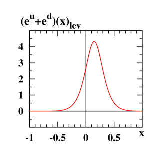
Figure 1: The contribution of the discrete level to $(e^{u}+e^{d})(x)$ as function of $x$.

The isoscalar combination $(e^{u}+e^{d})(x)$ contains a $\delta(x)$-singularity, as proven in Schweitzer:2003uy and independently shown in Wakamatsu:2003uu . A practical procedure to cope numerically with such a singularity in the $\chi$QSM was suggested in Schweitzer:2003uy , and used in Ohnishi:2003mf to confirm numerically the existence of the $\delta(x)$-singularity. In this Section we present an independent study, which will confirm the findings of Ref. Ohnishi:2003mf . Hereby we shall focus on the demonstration that the involved numerical calculation is well under control.

The contribution of the discrete level to $(e^{u}+e^{d})(x)$ as well as to any quantity in the model UV-finite. It can be computed by directly solving the eigenvalue problem (13) for the discrete level state Diakonov:1996sr , or by using the method described below. The result is shown in Fig. 1.

The continuum contribution can be computed in two ways, which follow from Eqs. (15, 16) (and to which we shall, for simplicity, continue referring as sums over occupied and non-occupied states), namely

$$(e^{u}+e^{d})(x)_{\rm cont,\,reg}=N_{c}M_{\rm N}\sum\limits_{E_{n}<0}\langle n|\gamma^{0}\delta(xM_{\rm N}-\hat{p}^{3}-E_{n})|n\rangle_{\rm reg}$$ , (25)

$$=-\,N_{c}M_{\rm N}\sum\limits_{E_{n}>0}\langle n|\gamma^{0}\delta(xM_{\rm N}-\hat{p}^{3}-E_{n})|n\rangle_{\rm reg}$$ . (26)

It is quadratically UV-divergent and has to be regularized, as indicated in (15, 16) and (25, 26). The Pauli-Villars subtraction method is the only regularization known in the $\chi$QSM which preserves all general properties of distribution functions (QCD sum rules, positivity, etc.) Diakonov:1996sr .

In order to regularize the continuum contribution and to ensure the equivalence of the summations over occupied and non-occupied states in Eqs. (25, 26), see Schweitzer:2003uy for a detailed discussion, two Pauli-Villars subtractions are necessary

$$(e^{u}+e^{d})(x)_{\rm cont,\,reg}=(e^{u}+e^{d})(x,M)_{\rm cont}-\alpha_{1}(e^{u}+e^{d})(x,M_{1})_{\rm cont}-\alpha_{2}(e^{u}+e^{d})(x,M_{2})_{\rm cont}$$ (27)

with

$$\alpha_{1}=\frac{M}{M_{1}}\;\frac{M_{2}^{2}-M^{2}}{M_{2}^{2}-M_{1}^{2}}\;\;,\;\;\;\alpha_{2}=-\frac{M}{M_{2}}\;\frac{M_{1}^{2}-M^{2}}{M_{2}^{2}-M_{1}^{2}}\;\;,\;\;\;M_{2}>M_{1}>M\;.$$ (28)

The values for the $M_{i}$ are fixed by regularizing the model expressions for the pion decay constant $f_{\pi}$ and the vacuum quark condensate $\langle\bar{\psi}\psi\rangle$ which are given in the effective theory (9) by the (Euclidean) loop integrals

$$f_{\pi}^{2}=\int\!\frac{{\rm d}^{4}p_{\mbox{\tiny E}}}{(2\pi)^{4}}\,\frac{4N_{c}M^{2}}{(p_{\mbox{\tiny E}}^{2}+M^{2})^{2}}\biggl{|}_{\rm reg}\;,\;\;\;\langle\bar{\psi}\psi\rangle\equiv\langle{\rm vac}|(\bar{\psi}_{u}\psi_{u}+\bar{\psi}_{d}\psi_{d})|{\rm vac}\rangle=-\int\!\frac{{\rm d}^{4}p_{\mbox{\tiny E}}}{(2\pi)^{4}}\,\frac{8N_{c}M}{p_{\mbox{\tiny E}}^{2}+M^{2}}\biggl{|}_{\rm reg}\;.\;\;\;$$ (29)

The model expression for the pion decay constant is regularized and its phenomenological value $f_{\pi}=93\,{\rm MeV}$ is reproduced by a single Pauli-Villars subtraction with $M_{1}=556\,{\rm MeV}$. Two subtractions analog to (27, 28) are needed to regularize the model expression for the quark vacuum condensate (29). In order to reproduce the phenomenological value $\langle\bar{\psi}\psi\rangle=-(280\pm 30)^{3}\,{\rm MeV}^{3}$ quoted in Gasser:1982ap one should use $M_{2}=(2.1^{+1.1}_{-0.7})\,{\rm GeV}$. For reasons which we will explain below a small value of $M_{2}$ is preferable, and we choose $M_{2}=986{\rm MeV}$ which yields $\langle\bar{\psi}\psi\rangle=-(220\,{\rm MeV})^{3}$. This is sufficiently close to the phenomenological value — considering the typical accuracy of the model.

In order to evaluate $(e^{u}+e^{d})(x)$ we use the following procedure Diakonov:1997vc . For the numerical calculation the Hamiltonian (13) is expressed and diagonalized in the basis of the eigenstates of the free Hamiltonian. The spectrum of (13) is discretized by placing the soliton in a finite but sufficiently large spherical box of the size $R_{\rm box}$ and imposing appropriate boundary conditions Kahana:1984be . The spectrum is made finite by cutting off quark momenta above some large numerical cutoff $\Lambda_{\rm num}$ chosen much larger than any other (physical or numerical) scale involved in the problem. We use $R_{\rm box}=(8-12)\,{\rm fm}$ and $\Lambda_{\rm num}=(8-9)\,{\rm GeV}$.

To compute the continuum contribution we introduce an intermediate regularization for any of the contributions in Eq. (27) schematically as

$$(e^{u}+e^{d})(x,M_{i})=N_{c}M_{\rm N}\biggl{[}\sum\limits_{n}\langle n|\gamma^{0}\delta(xM_{\rm N}-\hat{p}^{3}-E_{n})|n\rangle\;R(E_{n},\,\Lambda)\biggr{]}_{M_{i}}\;$$ (30)

where it is understood that the expression in squared brackets is to be evaluated with the Hamiltonian (13) if $M_{i}=M$, or with Hamiltonians analog to (13) but with $M$ replaced by $M_{1}$ or $M_{2}$, and where vacuum subtraction is implied. In (30) $R(\omega,\,\Lambda)$ is a smooth regulator function with $R(0,\,\Lambda)=1$ and $R(\omega,\,\Lambda)\to 0$ for $|\omega|\to\infty$. The intermediate cutoff $\Lambda$ must satisfy $M_{i}\ll\Lambda\ll\Lambda_{\rm num}$. It is due to this condition that we prefer a low value of $M_{2}$, see above. In practice we use $\Lambda\sim(3-6)\;{\rm GeV}$. The regulator function can be chosen to be of e.g. Gaussian or Wood-Saxon type. The dependence on $\Lambda$ and the choice of $R$ is removed at the end of the calculation by an extrapolation procedure.

It is convenient to turn (30) into a spherically symmetric form by replacing $\hat{p}^{3}\to{\bf u}\cdot\hat{\bf p}$ where ${\bf u}$ is a unit vector. (We recall that the 3-direction was singled out arbitrarily by choosing the spatial component of the light-like vector $n$ in (1) along that axis.) Averaging over the possible orientations of ${\bf u}$ yields

$$(e^{u}+e^{d})(x,M_{i})=N_{c}M_{\rm N}\biggl{[}\sum\limits_{n}\langle n|\gamma^{0}\;\frac{1}{2|\hat{\bf p}|}\,\Theta(|\hat{\bf p}|-|xM_{\rm N}-E_{n}|)|n\rangle\;R(E_{n},\,\Lambda)\biggr{]}_{M_{i}}\;.$$ (31)

As we work in a discrete basis the expression (31) is a discontinuous function of $x$ due to the appearance of the $\Theta$-function, and would become continuous only in the infinite volume limit. Rather than trying to take this limit numerically, which would be a time-consuming procedure, one may instead smear the expression in (31) by convoluting it with a narrow Gaussian as

$$(e^{u}+e^{d})(x,M_{i})=\frac{N_{c}M_{\rm N}}{\gamma\pi^{1/2}}\int{\rm d}x^{\prime}\,e^{-(x-x^{\prime})^{2}\gamma^{-2}}\;\biggl{[}\sum\limits_{n}\langle n|\gamma^{0}\;\frac{1}{2|\hat{\bf p}|}\,\Theta(|\hat{\bf p}|-|x^{\prime}M_{\rm N}-E_{n}|)|n\rangle\;R(E_{n},\,\Lambda)\biggr{]}_{M_{i}}\;.$$ (32)

In the limit $\gamma\to 0$ one recovers the original expression (31). The parameter $\gamma>0$ has to be chosen such that it is, on the one hand, sufficiently large compared to the typical splitting of energy levels in the discretized spectrum, and on the other hand, sufficiently small such that the “smeared function” is still a good approximation to the true result. For our box sizes $\gamma=0.1$ is adequate Diakonov:1997vc . In the end of the day the smearing can be removed by a deconvolution procedure, though in practice one finds that continuous functions are sufficiently well approximated by (32).

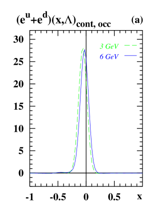
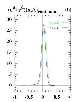
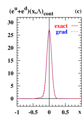
Figure 2: The continuum contribution to $(e^{u}+e^{d})(x)$ as function of $x$. (a) The result from the sum over occupied levels (25) for different values of the intermediate cutoff $\Lambda$. (c) The same as (b) but from the sum over non-occupied levels (26). (d) Solid line: the final result obtained after the extrapolation $\Lambda\to\infty$. Dotted line: the result from the gradient expansion Schweitzer:2003uy , see text.

It is precisely the smearing procedure which enables one to cope numerically with a $\delta$-function-type singularity. In fact, the smearing trick, turns the $\delta(x)$-contribution in $(e^{u}+e^{d})(x)$ into a narrow-Gausssian of a well-defined width $\gamma$ centered around $x=0$. Using the self-consistent profile from Weiss:1997rt which yields $1140\,{\rm MeV}$ for the soliton energy and the above described parameters we obtain for the regularized continuum contribution $(e^{u}+e^{d})(x,\Lambda)_{\rm cont}$ for the intermediate cutoffs $\Lambda=3$ and $6\,{\rm GeV}$ the results shown in Figs. 2a and b.

The results depend on whether one sums over occupied, Eq. (25), or non-occupied, Eq. (26), states and on the intermediate cutoff $\Lambda$. However, after extrapolating $\Lambda\to\infty$ both formulae (25) and (26) yield within a numerical accuracy of $1\%$ the same result, which is shown in Fig. 2c as solid line.

V The origin of the $\delta(x)$-singularity in $(e^{u}+e^{d})(x)$

Having convinced ourselves that one obtains for the continuum contribution of $(e^{u}+e^{d})(x)$ the same result, irrespective whether one computes it by means of (25) or (26), we have confidence in our numerical results, and are in the position to address the question: What precisely gives rise to the $\delta(x)$-singularity in $(e^{u}+e^{d})(x)$ in the $\chi$QSM?

As there is apparently no $\delta(x)$-term in the level part, see Fig. 1, one has to focus on the continuum contribution. The continuum contribution (25) or (26), is given in the gradient expansion by Schweitzer:2003uy

$$(e^{u}+e^{d})(x)_{\rm cont}=C\;\delta(x)+{\cal O}(\nabla U)\;,\;\;\;C=\langle\bar{\psi}\psi\rangle\int\!{\rm d}^{3}{\bf r}\;\biggl{(}\cos P(r)-1\biggr{)}\;,$$ (33)

where ${\cal O}(\nabla U)$ denotes terms which (i) contain one or more gradients of the chiral field $U$, i.e.  are suppressed in a chiral expansion, and (ii) are regular functions of $x$.

The result (33) is remarkable for two reasons. First, the coefficient $C$ of the $\delta(x)$-function can be computed exactly. Second, the quadratic and logarithmic divergences appearing in $C$ can be reexpressed in terms of $\langle\bar{\psi}\psi\rangle$ Schweitzer:2003uy .

It is is interesting to confront (33) which describes the singular part of $(e^{u}+e^{d})(x)$ in the gradient expansion exactly with our numerical result. For that we evaluate $C$ using the same Pauli-Villars masses, i.e.  $\langle\bar{\psi}\psi\rangle=-(220\,{\rm MeV})^{3}$, and the same self-consistent profile $P(r)$ as in the numerical calculation which yields

$$C_{\rm here}=4.88\;.$$ (34)

(The introduced index “here” reminds that this result holds for the Pauli-Villars masses used here, in this calculation.) Moreover, we smear the $\delta(x)$-function according to (32) with the same parameter $\gamma=0.1$ as used in the numerics. In this way we obtain the result shown as dashed line in Fig. 2c.

The impressive agreement in Fig. 2c fully confirms the findings of Ref. Schweitzer:2003uy that the $\delta(x)$-contribution in the $\chi$QSM originates solely from the leading order of the gradient expansion where it is related to the quark vacuum condensate. Fig. 2c also shows that the regular contribution to the continuum part of $(e^{u}+e^{d})(x)$ is small (on the scale in Fig. 2c). We observed similar agreements by varying the numerical parameters (Pauli-Villars masses $M_{i}$, profile $P(r)$, $\gamma$, etc.). These observations illustrate the utility of the gradient expansion as a powerful tool to control the numerics.

Let us report the following detail which further increases our faith into the quality of the numerics. In order to achieve the satisfactory agreement in Fig. 2c we considered the finite size of the spherical box used in the numerics, and integrated in (33) over the radial component $r=|{\bf r}|$ only up to $r=R_{\rm box}=12\,{\rm fm}$ which gave the result in (34). In the chiral limit the profile function behaves as $P(r)=A/r^{2}$ at large $r$, where $A$ is related to the isovector axial coupling constant $g_{A}$ by $A=(3g_{A})/(8\pi f_{\pi}^{2})$. In practice the asymptotics sets in already for $r\gtrsim 3\,{\rm fm}$ Weiss:1997rt . Thus, the finite size effect for the coefficient $C$ in (33) is

$$\delta C=\langle\bar{\psi}\psi\rangle\;4\pi\int_{R_{\rm box}}^{\infty}\!\!{\rm d}r\;r^{2}\biggl{(}\cos P(r)-1\biggr{)}=-\,\langle\bar{\psi}\psi\rangle\;\frac{2\pi\,A^{2}}{R_{\rm box}}\;.$$ (35)

The finite size effect slowly vanishes with increasing box size. For $R_{\rm box}=12\,{\rm fm}$ one has $\delta C_{\rm here}=0.196$, i.e. the result for $C_{\rm here}$ in (34) is about $4\%$ smaller compared to its infinite volume limit. Neglecting this effect would yield a clearly visible mismatch in Fig. 2c. Thus, as a byproduct we see that finite box size effects in our calculation are of the order of magnitude of a few percent, which is acceptable considering the typical model accuracy.

Thus, besides confirming numerically the presence of a $\delta(x)$-contribution in $(e^{u}+e^{d})(x)$ as was done previously in Ohnishi:2003mf , we furthermore have numerically confirmed the fact that the coefficient $C$ of the $\delta(x)$-function can be computed exactly using gradient expansion Schweitzer:2003uy . This is of importance because only the gradient expansion allows to relate $C$ to the quark vacuum condensate.

The exact prediction for the coefficient $C$ in the $\chi$QSM is therefore

$$C_{\rm exact}=10.5^{+3.7}_{-3.1}$$ (36)

using the self-consistent profile Weiss:1997rt and the phenomenological value $\langle\bar{\psi}\psi\rangle=-(280\pm 30)^{3}\,{\rm MeV}^{3}$ Gasser:1982ap whose uncertainty yields to the error shown in (36).

We remark that in Ohnishi:2003mf , where the Pauli-Villars masses were fixed to reproduce $\langle\bar{\psi}\psi\rangle=-(280\,{\rm MeV})^{3}$, the result $C\simeq 9.9$ was obtained numerically. This is in good agreement with the central value of (36) and the small discrepancy, apart from numerical uncertainties (finite box size effects), is due to the slightly different value of the constituent mass $M=375\,{\rm MeV}$ used in Ohnishi:2003mf , which yields a somehow different self-consistent profile. We checked that using larger values of $M_{2}\sim 1.5\,{\rm GeV}$ we are able to reproduce larger values of $C$. The price to pay for that is, however, a worse numerical stability because then the required hierarchy $M_{i}\ll\Lambda\ll\Lambda_{\rm num}$ holds less satisfactorily, unless one increases $\Lambda$ and $\Lambda_{\rm num}$ accordingly from which we refrained being limited by the computing resources available to us.

Having established the presence of a $\delta(x)$-type-singularity in $(e^{u}+e^{d})(x)$, confirming thereby the findings of Ohnishi:2003mf , we now turn to the task of computing the regular part of the continuum contribution.

VI Calculation of $x(e^{u}+e^{d})(x)$

Being interested in the regular part of the continuum contribution to $(e^{u}+e^{d})(x)$ the method of Sec. IV is not adequate. The smearing trick, which allows to visualize the delta-function, is of disadvantage in this case. It turns the $\delta(x)$-function into a Gaussian that penetrates into the regions $x\neq 0$ and dominates there over the regular part, Fig. 2c. Thus, a reliable computation of the regular part requires a different technic. Here we shall compute $x(e^{u}+e^{d})(x)$ where the $\delta(x)$ drops out. (Due to the smearing procedure (32) computing $x(e^{u}+e^{d})(x)$ is, of course, not the same as computing $(e^{u}+e^{d})(x)$ and multiplying the result by $x$.)

First we have to clarify how to regularize $x(e^{u}+e^{d})(x)$. It is worth to reconsider this point because $x(e^{u}+e^{d})(x)$ and $(e^{u}+e^{d})(x)$ differ by the appearance of a $\delta(x)$-term. As shown in Schweitzer:2003uy , the double subtraction (27, 28) is needed to make finite the coefficient of the $\delta(x)$-function. But is it also necessary to regularize $x(e^{u}+e^{d})(x)$? It is worth to reconsider this point: one could save a lot of computing time, if no or only one subtraction were necessary.

By going step by step through the Eqs. (32-40) of Ref. Schweitzer:2003uy , one believes, at a first impression, that a single subtraction (corresponding to (27, 28) for $M_{2}\to\infty$) is enough to remove from $x(e^{u}+e^{d})(x)$ a quadratic divergence and restore the equivalence of summations over occupied and non-occupied levels Schweitzer:2003uy . However, such a conclusion is premature and we show here that a double subtraction is adequate.

In order to illustrate why we integrate $x(e^{u}+e^{d})(x)$ from (25, 26) over $x$, explore the model equations of motion, and arrive at expressions for the continuum contribution to the second moment of $(e^{u}+e^{d})(x)$ which read Schweitzer:2003uy

$$\int{\rm d}x\,x(e^{u}+e^{d})(x)_{\rm cont} = \frac{N_{c}M}{2M_{\rm N}}\sum_{E_{n}<0}\langle n|(U+U^{\dagger})|n\rangle_{\rm reg}$$ (37)

$$= -\frac{N_{c}M}{2M_{\rm N}}\sum_{E_{n}>0}\langle n|(U+U^{\dagger})|n\rangle_{\rm reg}\;.$$ (38)

Clearly, the difference of the two expressions in (37) and (38) must be zero, i.e.  one expects

$$A_{\rm reg}\equiv\frac{N_{c}M}{2M_{\rm N}}\sum_{n\,\rm all}\langle n|(U+U^{\dagger})|n\rangle_{\rm reg}=\frac{N_{c}M}{M_{\rm N}}\;{\rm Sp}\,\Biggl{[}\frac{U+U^{\dagger}}{2}-1\Biggr{]}_{\rm reg}\stackrel{{\scriptstyle!}}{{=}}0\;.$$ (39)

Here ${\rm Sp}$ denotes the functional trace which can be saturated by any complete set of functions, ${\rm Sp}[\,\dots\,]=\sum_{n}\langle n|\dots|n\rangle$ being one example. Notice that the “$-1$” in Eq. (39) is due to the explicitly included vacuum subtraction.

In the numerical calculation the expression for $A_{\rm reg}$ is evaluated with an intermediate regularization, see Eq. (30), such that in the intermediate step we are interested in the following expression

$$A(\Lambda,M)=\frac{N_{c}M}{M_{\rm N}}\;{\rm Sp}\,\Biggl{[}\frac{U+U^{\dagger}}{2}\,R(H,\,\Lambda)-R(H_{0},\,\Lambda)\Biggr{]}\;.$$ (40)

We evaluate $A(\Lambda,M)$ in Eq. (40) in gradient expansion where $R(H,\,\Lambda)=R(H_{0},\,\Lambda)+{\cal O}(\nabla U)$ holds, and saturate ${\rm Sp}[\,\dots\,]=$ $\int\frac{{\rm d}^{3}{\bf k}}{(2\pi)^{3}}\langle{\bf k}|{\rm tr}\,\dots|{\bf k}\rangle$ in the spectrum of the free momentum operator where ${\rm tr}$ denotes the trace over Dirac- and flavour-indices. As positive and negative energies must be regularized equally, i.e. $R(\omega,\Lambda)=R(-\omega,\Lambda)$, we obtain:

$$A(\Lambda,M)=\frac{8N_{c}M}{M_{\rm N}}\;\int\!{\rm d}^{3}{\bf x}\,(\cos P(r)-1)\;\int\!\frac{{\rm d}^{3}{\bf k}}{(2\pi)^{3}}\,R(\sqrt{{\bf k}^{2}+M^{2}},\Lambda)\;.$$ (41)

We recognize, most easily by employing a definite regulator such as e.g. a simple Gaussian $R(\omega,\Lambda)=\exp(-\omega^{2}/\Lambda^{2})$, that $A(\Lambda,M)$ has a cubic and a linear divergence for $\Lambda\to\infty$. The double subtraction (27, 28) not only removes these divergences but also restores the equivalence of the summations over occupied or non-occupied states, i.e.

$$A_{\rm reg}\equiv\lim\limits_{\Lambda\to\infty}A(\Lambda)=0\;,\;\;\;\mbox{where}\;\;\;A(\Lambda)\equiv A(\Lambda,M)-\alpha_{1}A(\Lambda,M_{1})-\alpha_{2}A(\Lambda,M_{2})\;.$$ (42)

One can convince oneself similarly as done in Schweitzer:2003uy that higher orders in $\nabla U$ omitted in (41) do not spoil the above argumentation. Thus, $x(e^{u}+e^{d})(x)$ must be regularized exactly in the same way as $(e^{u}+e^{d})(x)$ according to (27, 28).

The reason why the calculation in Eqs. (32-40) of Schweitzer:2003uy lead us to the premature conclusion that a single subtraction could be sufficient is because here and in Schweitzer:2003uy different matrix elements were evaluated in gradient expansion, namely

$$\langle n|E_{n}\gamma^{0}|n\rangle\biggl{|}_{\mbox{\footnotesize used in \cite[cite]{\@@bibref{Authors Phrase1YearPhrase2}{Schweitzer:2003uy}{\@@citephrase{(}}{\@@citephrase{)}}}}}\;\;\stackrel{{\scriptstyle\rm eom}}{{=}}\;\frac{1}{2}\,\langle n|\{\hat{H},\gamma^{0}\}|n\rangle=\frac{1}{2}\,M\,\langle n|(U+U^{\dagger})|n\rangle\biggl{|}_{\mbox{\footnotesize used here}}$$ (43)

which are connected by equations of motion (eom). The latter are, of course, not respected in a truncated expansion. Another example that the gradient expansion yields results at variance with eom is documented in Sec. 7 of Ref. Diakonov:1996sr .

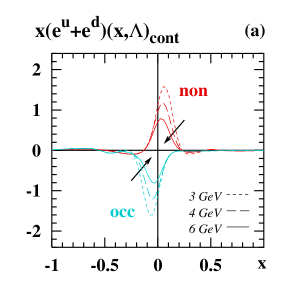
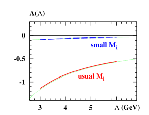
Figure 3: The continuum contribution to $x(e^{u}+e^{d})(x)$ as function of $x$ from sums over occupied (“occ”) and non-occupied (“non”) levels for different intermediate cutoffs $\Lambda$. The arrows indicate the tendency of the curves with increasing cutoff.

Figure 4: The difference $A(\Lambda)$ defined in (39) as function of the intermediate cutoff $\Lambda$. It must vanish for $\Lambda\to\infty$ according to (42). The thick curves are the numerical results. Solid: for “usual” Pauli-Villars masses used throughout. Dashed: for a set of smaller masses $M_{1}=389\,{\rm MeV}$ and $M_{2}=700\,{\rm MeV}$. The thin curves are the respective analytical results from Eq. (41).

Having clarified the issue of regularization we turn to the numerical evaluation. At first glance one may have the impression that different expressions exist, namely

$$x(e^{u}+e^{d})(x) = xM_{\rm N}N_{c}\sum\limits_{n\;\rm occ}\langle n|\gamma^{0}\delta(xM_{\rm N}-\hat{p}^{3}-E_{n})|n\rangle_{\rm reg}$$

$$= N_{c}\sum\limits_{n\;\rm occ}\langle n|\gamma^{0}\delta(xM_{\rm N}-\hat{p}^{3}-E_{n})\,(\hat{p}^{3}+E_{n})\,|n\rangle_{\rm reg}$$

and analog expressions with summations over non-occupied states. However, it is gratifying to observe that after averaging over directions either of these expressions just yields $x$ times the result in Eq. (31).

The numerical procedure of Sec. IV yields for $x(e^{u}+e^{d})(x,\Lambda)_{\rm cont}$ the results shown in Fig. 4. We make two interesting observations. First, compared to the huge effect of the smeared out $\delta(x)$-function in Fig. 2 the regular contribution is small. Second, the results for the sums over positive and negative energy states exhibit a tendency with increasing intermediate cutoff $\Lambda$ to converge slowly towards a common result. However, this convergence is remarkably slow, and the numerical stability of a $\Lambda\to\infty$ extrapolation is poor, especially for small $|x|\lesssim 0.2$.

The slow convergence can be understood as follows. We compute the moment $\int{\rm d}x\,x(e^{u}+e^{d})(x)_{\rm cont}$ summing over respectively occupied, Eq. (37), and non-occupied, Eq. (38), states, and take the difference. This yields the $A(\Lambda)$ defined in Eq. (42), which is expected to be zero in the limit $\Lambda\to 0$. The numerical results for $A(\Lambda)$ for $3\,{\rm GeV}\leq\Lambda\leq 6\,{\rm GeV}$ are shown in Fig. 4. We see that $A(\Lambda)$ tends to zero with increasing $\Lambda$ but very slowly. (We checked that one obtains within few percent the same result from integrating the curves for $x(e^{u}+e^{d})(x)_{\rm cont}$ in Fig. 4.)

This slow vanishing of the “anomaly” (in the sense of Goeke:2000wv ) $A(\Lambda)$ is, in fact, precisely what we expect. In order to see that, we evaluate the theoretical expression (41) for $A(\Lambda)$ in the same way as done in the numerics, namely for the Wood-Saxon regulator

$$R(\omega,\Lambda)=\frac{1}{1+\exp[(|\omega|-\Lambda)/\varepsilon]}$$ (45)

with the box-size dependent width $\varepsilon=4/R_{\rm box}$ (here $R_{\rm box}=12\,{\rm fm}$), and integrate in spherical coordinates over ${\bf k}$ up to $|{\bf k}|\leq\Lambda_{\rm num}=8.9\,{\rm GeV}$. The result is shown in Fig. 4 as dashed line, and we observe again an impressive agreement of the analytical and numerical results.

To test further the theoretical result (41) we repeated the calculation with $M_{1}=389\,{\rm MeV}$ and $M_{2}=700\,{\rm MeV}$. With smaller (compared to the “usual” ones fixed in the sequence of Eq. (29) and used throughout) Pauli-Villars masses one subtracts “more”. (The opposite is evident, for $M_{1,2}\to\infty$ one recovers unregularized, divergent expressions.) Therefore, continuum contributions and consequently $A(\Lambda)$ are smaller. Also in this case the analytical and numerical results agree remarkably, see Fig. 4.

It happens that $A(\Lambda)$ is much larger then the continuum contribution whose computation it hampers, namely (in the numerator of the undesired, anomalous terms cancel out)

$$\left|\frac{\int{\rm d}x\,x(e^{u}+e^{d})(x,\Lambda)_{\rm cont,\,occ}-\int{\rm d}x\,x(e^{u}+e^{d})(x,\Lambda)_{\rm cont,\,non}}{\int{\rm d}x\,x(e^{u}+e^{d})(x,\Lambda)_{\rm cont,\,occ}+\int{\rm d}x\,x(e^{u}+e^{d})(x,\Lambda)_{\rm cont,\,non}}\right|\gtrsim\cases{10&for usual Pauli-Villars masses\cr 3&for small Pauli-Villars masses}$$ (46)

for $3\,{\rm GeV}\leq\Lambda\leq 6\,{\rm GeV}$. The result (46) indicates that, the better the condition $M_{i}\ll\Lambda\ll\Lambda_{\rm num}$ is realized, the less the undesired anomalous difference is disturbing. Thus, were we able to use intermediate cutoffs satisfying more convincingly the condition $\Lambda\gg M_{i}$, it would be possible to perform reliably the extrapolation $\Lambda\to\infty$. However, here we are restricted, since a numerical cutoff $\Lambda_{\rm num}$ of substantially more than $10\,{\rm GeV}$ would require unacceptably long computing times. Unfortunately, this means that with justifiable effort one cannot establish the equivalence of summations over occupied and non-occupied levels.

The calculation in Eqs. (32-40) of Schweitzer:2003uy reveals how this contribution, which only slowly vanishes with increasing $\Lambda$, is distributed in $x$. The anomalous terms appear at $x<0$ ($x>0$) when computing $x(e^{u}+e^{d})(x,\Lambda,M_{i})$ from occupied (non-occupied) states. Due to the smearing procedure, however, the effects of the anomalous terms penetrate also in the respectively opposite $x$-regions, and yield the picture in Fig. 4.

¿From this observation it is clear how one can evaluate $x(e^{u}+e^{d})(x)$. We have to switch off the smearing, and for $x>0$ ($x<0$) we have to sum over occupied (non-occupied) states.

The observation that for $x>0$ ($x<0$) the sums over occupied (non-occupied) states converge faster than in the opposite $x$-regions was already noticed in Diakonov:1997vc . Still, in all examples encountered so far, the convergence in those slower-convergence-$x$-regions was fast enough in order to establish reliably the equivalence of results from summations over occupied and non-occupied states Diakonov:1997vc ; Weiss:1997rt ; Pobylitsa:1998tk ; Goeke:2000wv ; Schweitzer:2001sr ; Ossmann:2004bp . Here we face for the first time the situation where this is not possible, which is not surprizing as it is also the first time one has to deal with Pauli-Villars-masses of ${\cal O}(1\,{\rm GeV})$, and we are forced to give up this strong test of the numerical results.

The price to pay for giving up the smearing step (32) is less serious. One may turn discontinuous results into final, continuous ones, see below.

Fig. 5a shows the results for the continuum contribution to the antiquark distribution, $x(e^{\bar{u}}+e^{\bar{d}})(x)_{\rm cont,\,non}$ (i.e. $x(e^{u}+e^{d})(x)_{\rm cont}$ at negative $x$) obtained from the sum over non-occupied states without smearing, for $\gamma\to 0$ in (32). The discountinuous nature of the curve is apparent (we connected the points to guide the eye). It is remarkable that our results practically do not depend on the intermediate cutoff $\Lambda$. In other words, we observe a very fast convergence in $\Lambda$. It is clear that whatever procedure we use to “smooth” the curve, it will introduce larger numerical uncertainties then the extrapolation in $\Lambda$, and therefore refrained from performing the latter. The solid curve in Fig. 5a shows the final, smoothened curve obtained from fitting the discontinuous curves.

Fig. 5b shows the corresponding results for $x(e^{u}+e^{d})(x)_{\rm cont,\,occ}$ obtained from the sum over occupied states. Also here we observe a stable convergence in $\Lambda$, except for very small $x\sim 0.05$, where anyway the finite box method is not reliable, and the large-$N_{c}$ approach not applicable Diakonov:1996sr ; Diakonov:1997vc . The solid curve in Fig. 5b shows the final result obtained from fitting the discontinuous curves. (Since the continuum contribution to the quark distribution is far smaller than to the antiquark distribution, we computed it with a more coarse-grained resolution in $x$.)

What about the respective slow-convergence-$x$-regions? Here, without smearing, one observes fluctuations similar to that in Fig. 5, but two orders of magnitude larger, which are due to the anomalous terms, see the discussion above.

Having switched of smearing, we could have equally computed $(e^{u}+e^{d})(x)$ (since now computing $x(e^{u}+e^{d})(x)$ or computing $(e^{u}+e^{d})(x)$ and multiplying by $x$, of course, commutes). Still it is preferable to calculate $x(e^{u}+e^{d})(x)$, and the reason is evident from Fig. 5. With increasing $x$ the $\Theta$-functions in (31) allow to include more discrete states, and the fluctuations due to the discrete basis diminish. And vice versa, at small $x$ only few long-wave-length states contribute, which enhances the fluctuations (and is the reason why here one is particularly sensitive to details of the finite box method, as mentioned above). Weighting the function by $x$ suppresses the fluctuations in the small-$x$ region yielding a less fluctuating curve which can be “smoothened” more reliably, as is demonstrated by Fig. 5.

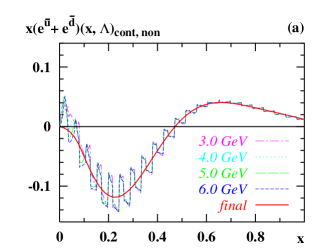
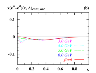
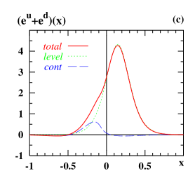
Figure 5: The regular continuum contributions to (a) $x(e^{\bar{u}}+e^{\bar{d}})(x)$, and (b) $x(e^{u}+e^{d})(x)$ as functions of $x$ for the intermediate cutoffs $\Lambda=3,\,4,\,5$ and $6\,{\rm GeV}$, and the respective final, smoothened results. (c) The total result for the regular part of $(e^{u}+e^{d})(x)$ as function of $x$, and how it is decomposed of the discrete level and continuum contributions.

The final result for the regular part of $(e^{u}+e^{d})(x)$ is shown in Fig. 5c. For completeness we show how it is composed of the contributions from the discrete level, Fig. 1, and the continuum contribution, Figs. 5a and b. (In the smoothening step yielding the final (solid) curves in Figs. 5a and b we have build in the constrain that the regular part to the continuum contribution behaves as $(e^{u}+e^{d})(x)_{\rm cont}\to{\rm const}\,$ for $x\to 0$.)

As can be seen from Fig. 5c, the regular continuum contribution to $(e^{u}+e^{d})(x)$ is small compared to the discrete level contribution which dominates the final result. Although we could not check the equivalence of the regular continuum results from summations over occupied and non-occupied states, we still were able to clearly demonstrate that the numerical calculation is well under control, which gives confidence into the final results.

VII Calculation of $(e^{u}-e^{d})(x)$

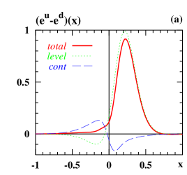
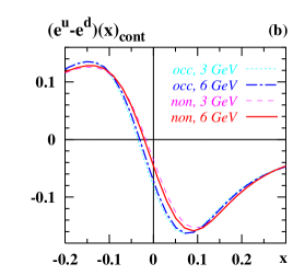
Figure 6: (a) The total result for $(e^{u}-e^{d})(x)$ as function of $x$, and how it is decomposed from the discrete level and continuum contributions. (b) A detail on how the final result for the continuum contribution in Fig. 6a comes about: $(e^{u}-e^{d})(x,\Lambda)_{\rm cont}$ as function of $x$ for different intermediate cutoffs from sums over respectively the occupied and non-occupied states.

The flavour non-singlet combination $(e^{u}-e^{d})(x)$ appears only at subleading order in the $1/N_{c}$ expansion, when one includes “rotational” corrections. This flavour combination is UV-finite and does not need to be regularized. Fig. 6a shows the final result for $(e^{u}-e^{d})(x)$. It is also shown how the total result is decomposed of respectively the discrete level and continuum contributions.

We observe a fast and stable convergence of the continuum contribution $(e^{u}-e^{d})(x,\Lambda)_{\rm cont}$ with increasing intermediate cutoff $\Lambda$. This is demonstrated in Fig. 6b where only the region of strongest $\Lambda$-dependence around $|x|<0.3$ is shown. Notice that the different curves in Fig. 6b would be nearly indistinguishable on the scale of Fig. 6a. After the extrapolation $\Lambda\to\infty$ one obtains from the sums over respectively over occupied and non-occupied states, Eqs. (20) and (24), results which coincide to within an accuracy of about $1\%$.

The final result for $(e^{u}-e^{d})(x)$ shown in Fig. 6 reveals that it is a regular function of $x$. In particular, no $\delta(x)$-type singularity appears in this flavour combination.

In order to separate consistently different flavours, $e^{u}(x)$ and $e^{d}(x)$, it would be necessary to consider also rotational corrections to the leading large-$N_{c}$ structure $(e^{u}+e^{d})(x)$. Applying straight-forwardly the procedure described in Sec. III which lead to the expressions (15-24) one obtains rotational corrections to $(e^{u}+e^{d})(x)$ consisting only of incomplete double sums. This is a general feature encountered whenever one considers $1/N_{c}$-corrections in the model to those parton distribution functions which appear already at leading order of the large-$N_{c}$ expansion Schweitzer:2001sr . Below, when discussing the final results for $e^{a}(x)$, we shall follow the suggestion Wakamatsu:1998rx ; Ohnishi:2003mf to discard such terms.

VIII Discussion of results for $e^{a}(x)$ and sum rules

It is interesting to observe that $e^{a}(x)$ clearly respects the large-$N_{c}$ predictions for the flavour dependence, Eq. (II). The “large” flavour combination $(e^{u}+e^{d})(x)$ is indeed much larger than the “small” flavour combination $(e^{u}-e^{d})(x)$, see Fig. 8a. As a consequence one finds $e^{u}(x)\approx e^{d}(x)$ within an accuracy of about $30\,\%$, see Fig. 8b, which is precisely what one generically expects from next-to-leading order corrections in an $1/N_{c}$-expansion with $N_{c}=3$. The large-$N_{c}$ predictions are even more convincingly realized in the case of antiquarks, see Fig. 8c.

In order to gain some more intuition on the model results for $e^{a}(x)$ it is instructive to compare them to $f_{1}^{a}(x)$ computed in the same model Weiss:1997rt ; Pobylitsa:1998tk . The $\chi$QSM results for $f_{1}^{a}(x)$ agree to within an accuracy of about $30\%$ with parameterizations performed at comparably low scales GRV ; GRSV .

Figs. 8a-d show $xe^{a}(x)$ in comparison to $xf_{1}^{a}(x)$ for $a=u,\,d,\,\bar{u},\,\bar{d}$ at the low scale of the model. (In this figure it can be seen best that in the model parton distribution functions have a non-zero support also for $x>1$ where, however, they are proportional to $\exp(-{\rm const}\,N_{c}x)$ Diakonov:1996sr . Since our results refer to the large-$N_{c}$ limit, there is conceptually no problem. In practice, even for $N_{c}=3$ the distribution functions are negligibly small for $x>1$, see Fig. 8.)

It is remarkable that the $e^{a}(x)$ are sizeable only for $x\lesssim 0.5$, in contrast to the $f_{1}^{a}(x)$ which extend also to larger values of $x$. In the region of $x\lesssim 0.5$ the quark distributions $e^{q}(x)$ are about half the magnitude of the $f_{1}^{q}(x)$. However, the antiquark distributions $e^{\bar{q}}(x)$ and $f_{1}^{\bar{q}}(x)$ are of comparable magnitude.

This comparison is interesting also because it was shown that in the non-relativistic limit $e^{q}(x)$ and $f_{1}^{q}(x)$ coincide Efremov:2002qh ; Schweitzer:2003uy . In the $\chi$QSM, which is a relativistic model, one is far away from a non-relativistic scenario, see Figs. 8a and b.

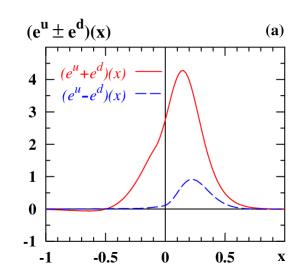
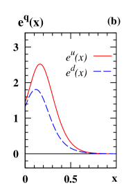
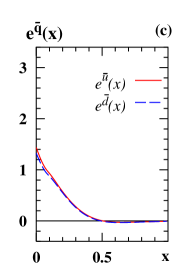
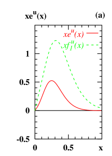
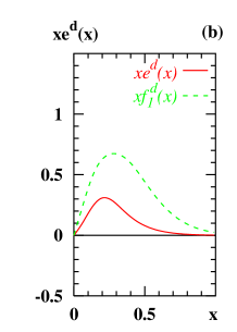
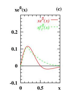
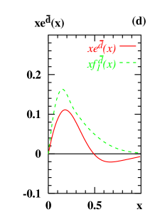
Figure 7: (a) Comparison of $(e^{u}+e^{d})(x)$ and $(e^{u}-e^{d})(x)$ as functions of $x$. (No attempt is made to indicate the $\delta(x)$-contribution in the flavour singlet case.) (b) The quark distributions $e^{u}(x)$ and $e^{d}(x)$. (c) The antiquark distributions $e^{\bar{u}}(x)$ and $e^{\bar{d}}(x)$.

Figure 8: The different flavours of $xe^{a}(x)$ as functions of $x$ in comparison to $xf_{1}^{a}(x)$ from the same model, Refs. Weiss:1997rt ; Pobylitsa:1998tk .

Next let us discuss the sum rules (5, 6) which were analytically proven to be satisfied in the model in Refs. Schweitzer:2003uy ; Wakamatsu:2003uu ; Ohnishi:2003mf . For the first moments we obtain here

$$\int_{-1}^{1}\!{\rm d}x\;(e^{u}+e^{d})(x)=1.76_{\rm lev}+0.11_{\rm cont,\,reg}+(4.88+0.196)_{\rm cont,\,sing}=6.95\,,$$ (47)

$$\int_{-1}^{1}\!{\rm d}x\;(e^{u}-e^{d})(x)=0.303_{\rm lev}+0.001_{\rm cont}=0.30\,,$$ (48)

where we indicate how the numbers are composed of respectively the discrete level, and the regular and singular continuum contributions (the last corrected for the finite box size effects we know, see Sec. V). The results are in agreement with phenomenology, see (5, 6). Notice, that the result in (47) is strongly sensitive to details of regularization. With the exact result for the coefficient $C$ we obtain $\int{\rm d}x\,(e^{u}+e^{d})(x)\simeq 12$, see Sec. V.

While the sum rules (5, 6) are formally satisfied in the model Schweitzer:2003uy ; Wakamatsu:2003uu ; Ohnishi:2003mf and numerically in satisfactory agreement with phenomenology one must admit a shortcoming. In QCD the sum rules (5, 6) are saturated solely by the $\delta(x)$-contribution, see Sec. II. In contrast to that in the model about $20\,\%$ of the result in (47) are due to the regular part of $(e^{u}+e^{d})(x)$, while the total result in (48) is due to the regular (and only) part of $(e^{u}-e^{d})(x)$.

Another shortcoming is that in the chiral limit to which our results refer the second moments (4) for $(e^{u}\pm e^{d})(x)$ vanish in QCD. Instead, we obtain in the model

$$\int_{-1}^{1}\!{\rm d}x\;x(e^{u}+e^{d})(x)=0.258_{\rm lev}-0.024_{\rm cont}=0.23\,,$$ (49)

$$\int_{-1}^{1}\!{\rm d}x\;x(e^{u}-e^{d})(x)=0.089_{\rm lev}-0.019_{\rm cont}=0.07\,.$$ (50)

These two shortcomings have the same origin.

Both, the fact that the sum rule (3) is saturated solely by the $\delta(x)$-contribution and the sum rule (4), follow from applying explicitly the QCD equations of motion. At this point the $\chi$QSM and actually any model is overburdened. Effective model approaches do not respect the QCD equations of motion, rather they satisfy the respective model equations of motion. Therefore it is not surprizing to observe such sum rules not to be satisfied literally. Still, one may explore model equations of motions and reinterpret the sum rules (3, 4) in the model terminology Schweitzer:2003uy ; Ohnishi:2003mf .

IX Comparison to previous calculations in the $\chi$QSM

The first (approximate) calculation of $e^{a}(x)$ in the $\chi$QSM was reported in Schweitzer:2003uy . There the regular part of $(e^{u}+e^{d})(x)$ was approximated by the discrete level contribution, and rotational corrections were discarded. The accuracy of these approximations was estimated to be within $30\,\%$. In fact, the (regular) continuum contributions are small compared to the respective discrete level contributions, see Figs. 5c and 6a, and the rotational correction $(e^{u}-e^{d})(x)\ll(e^{u}+e^{d})(x)$, see Sec. VIII. Thus, the estimates of Schweitzer:2003uy did indeed approximate $e^{a}(x)$ within the claimed accuracy. Of course, this became clear only after exact calculations were presented.

The first exact calculation of $e^{a}(x)$ in the $\chi$QSM was presented in Ohnishi:2003mf , and the present work confirms the results obtained there. The main quantitative difference between our work and Ohnishi:2003mf is that there it was possible to handle much larger Pauli-Villars masses (which requires, see Sec. IV, more computing power available in Ohnishi:2003mf ).

The choice of Pauli-Villars masses is relevant for the continuum contribution $(e^{u}+e^{d})(x)$. As a consequence of the larger Pauli-Villars masses in Ohnishi:2003mf an about two times larger coefficient of the $\delta(x)$-contribution was obtained. But the results for the regular contribution to $e^{a}(x)$ obtained here and in Ohnishi:2003mf practically agree. In fact, these results are strongly dominated by the discrete level contributions, see Figs. 5c and 6a, and at this point the slightly different value of the constituent mass $M=375\,{\rm MeV}$ used in Ohnishi:2003mf (compared to $M=350\,{\rm MeV}$ used here) is more decisive than the different choice of Pauli-Villars masses.

The present work extends in several aspects Ref. Ohnishi:2003mf , which was up to now the most detailed and complete study of $e^{a}(x)$ in this model.

• We have shown that the coefficient $C$ of the $\delta(x)$-term in $(e^{u}+e^{d})(x)$ can be determined exactly by means of an analytical calculation Schweitzer:2003uy .

• We have determined finite box size corrections for the coefficient $C$ of the $\delta(x)$-term in $(e^{u}+e^{d})(x)$.

• We demonstrated the equivalence of results obtained from summations over occupied and non-occupied states, wherever possible. (In Ohnishi:2003mf the equivalence was demonstrated only for the coefficient $C$.)

• Where this was not possible, namely for the regular continuum part of $(e^{u}+e^{d})(x)$, we were able to explain why, and to demonstrate that nevertheless the involved numerics is under analytical control.

In view of the complexity of the task — to deal numerically with a $\delta(x)$-term, to use a double Pauli-Villars subtraction with large Pauli-Villars masses — the present work provides an important supplement to Refs. Schweitzer:2003uy ; Wakamatsu:2003uu ; Ohnishi:2003mf .

X Comparison to results from other models

The distribution function $e^{a}(x)$ was studied also in other non-perturbative model-approaches, such as bag Jaffe:1991ra ; Signal:1996ct or spectator Jakob:1997wg models, as well as in 1+1 dimensional toy-models or perturbative one-loop model calculations Burkardt:1995ts ; Burkardt:2001iy . In Fig. 9 we compare our results to the MIT bag model calculation Jaffe:1991ra and the spectator model Jakob:1997wg .

In the bag model version used in Jaffe:1991ra the nucleon is assumed to consist of 3 non-interacting, massless quarks confined to the interior of a 3D spherical cavity (“bag”) by imposing appropriate covariant boundary conditions which model confinement and mimic gluonic effects. The model is relativistic. The flavour dependence is due to the assumed SU(2)${}_{\rm flavour}\times$SU(2)_spin spin-flavour-symmetry of the quark wave functions such that $e^{u}(x)=2\,{\rm e}(x)$ and $e^{d}(x)={\rm e}(x)$, and analogously for antiquarks, with ${\rm e}(x)$ as introduced in Jaffe:1991ra . There is no $\delta(x)$-contribution in the bag model, and since the quarks are massless, the $e^{a}(x)$ computed in Jaffe:1991ra correspond to $e^{a}_{\rm tw3}(x)$ in Eq. (2). Interestingly, the pure twist-3 (“interaction-dependent”) nature of this contribution is reflected in the bag model by the fact that $e^{a}(x)$ is due to bag-boundary effects. The sum rules (3, 4) are not satisfied in the bag model because the QCD equations of motion are modified in the bag Jaffe:1991ra , c.f. the discussion in the $\chi$QSM in Sec. VIII.

The bag gives also rise to antiquark distributions, however, to unphysical ones since the unpolarized antiquark distributions in the bag model violate positivity, i.e. in this model $f_{1}^{\bar{q}}(x)<0$ is found. Only valence quark distributions are considered to be physical Jaffe:1974nj . Keeping this mind, we plot also $e^{\bar{q}}(x)$ from the bag model in Fig. 9c and d.

In spectator models parton distribution functions are modelled by introducing a unity in the shape of $\sum_{n}|n\rangle\,\langle n|=1$ into the definition, here Eq. (1), where $\{|n\rangle\}$ is a complete set of intermediate states, and modelling this complete set of states by e.g. a diquark state. Hereby the diquark state can be taken to be, e.g., in a spin 0 or spin 1 state, which is referred to as respectively scalar and vector diquark. Both were considered in Jakob:1997wg which yields, in spite of the SU(2)${}_{\rm flavour}\times$SU(2)_spin spin-flavour-symmetry assumed also there, to a non-trivial flavour dependence in Figs. 9a, b. Antiquark distributions can be included by introducing more complex intermediate spectator states, but were not considered in Jakob:1997wg . Also the spectator model does not respect the sum rules (3, 4).

When comparing the different models of $e^{a}(x)$ in Fig. 9 one has to keep in mind that the low scales in the various models differ somehow. Bag model results refer to a scale of about $0.4\,{\rm GeV}$, spectator model results to about $0.5\,{\rm GeV}$, and the scale of $\chi$QSM results is roughly $0.6\,{\rm GeV}$, see Eq. (10).

The three models agree on that $e^{u}(x)$ is positive and sizeable for $x\lesssim 0.5$, see Fig. 9a, while $e^{d}(x)$ appears to be smaller (and exhibits in the spectator model even a remarkable zero around $x\sim 0.3$), see Fig. 9b. The $e^{\bar{q}}(x)$ are much larger in the $\chi$QSM model than in the bag model, see Figs. 9c and d. Only in the $\chi$QSM there is a $\delta(x)$-contribution at $x=0$ (no attempt was made to indicate this singularity in Fig. 9).

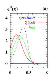
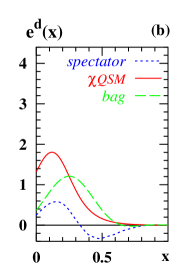
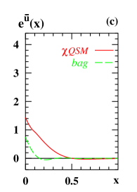
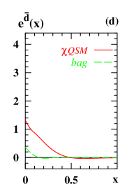
Figure 9: Comparison of predictions for $e^{a}(x)$ from different models. Solid line: $\chi$QSM, computed in this work. Dashed line: bag model Jaffe:1991ra . Dotted line: spectator model Jakob:1997wg .

XI Conclusions

A study of the distribution functions $e^{a}(x)$ in the $\chi$QSM was presented which completes previous works Schweitzer:2003uy ; Wakamatsu:2003uu ; Ohnishi:2003mf . Two particular features not encountered before in calculations of other parton distribution functions complicate the computation of $e^{a}(x)$ in the $\chi$QSM: the appearances of a $\delta(x)$-singularity and of quadratic UV-divergences whose regularization requires a double Pauli-Villars subtraction with a large second Pauli-Villars mass $M_{2}={\cal O}(1\,{\rm GeV})$. We have demonstrated in detail that in spite of these complications a reliable, controlled numerical calculation is possible. Our results confirm qualitatively and quantitatively previous calculations of $e^{a}(x)$ in the $\chi$QSM Schweitzer:2003uy ; Wakamatsu:2003uu ; Ohnishi:2003mf .

Moreover, our study reveals several interesting results. We have demonstrated that the coefficient $C$ of the $\delta(x)$-singularity in $(e^{u}+e^{d})(x)$ can be calculated analytically in the model Schweitzer:2003uy . As far we are aware this the only case where it is possible to compute exactly a (though admittedly unusual) contribution to a parton distribution function in the $\chi$QSM. This means that the coefficient $C$ of the $\delta(x)$-term is exactly proportional to the quark vacuum condensate, and thus ultimately connected to chiral symmetry breaking Schweitzer:2003uy .

Another interesting, but more technical byproduct of our study is that we have been able to quantify exactly the finite-box-size corrections to a quantity in the model, namely to the coefficient $C$ (which are of the order of few $\%$). This is also, to best of our knowledge, unique in the model.

The $\chi$QSM predicts $e^{u}(x)$ to be positive and sizeable — reaching half the size of $f_{1}^{u}(x)$ — in the region of $x\lesssim 0.5$, and $e^{d}(x)$ somehow smaller. Remarkably, in this region of $x$ the $e^{\bar{q}}(x)$ appear to be of similar magnitude as the $f_{1}^{\bar{q}}(x)$. Our predictions for the quark distributions $e^{q}(x)$ are in rough qualitative agreement with results from bag Jaffe:1991ra ; Signal:1996ct or spectator Jakob:1997wg models in which, however, no $\delta(x)$-contribution appears.

Here, following the practical point of view of Ref. Jaffe:1991ra , we computed $e^{a}(x)$ benefiting from a special property of this twist-3 quantity, which allows to define it in terms of quark fields only, and thus makes possible studies in models without explicit gluon degrees of freedom Jaffe:1991ra . However, by means of QCD equations of motion $e^{a}(x)$ can be reexpressed such that they explicitly depend on gluon fields. The question whether quark models, like the $\chi$QSM, are nevertheless able to provide useful estimates for $e^{a}(x)$, at least in certain regions of $x$, can be clarified only by experiment.