The High Density Region of QCD from an Effective Model

Abstract:

We study the high density region of QCD within an effective model obtained in the frame of the hopping parameter expansion and choosing Polyakov-type loops as the main dynamical variables representing the fermionic matter. This model still shows the so-called sign problem, a difficulty peculiar to non-zero chemical potential, but it permits the development of algorithms which ensure a good overlap of the simulated Monte Carlo ensemble with the true one.

We review the main features of the model and present results concerning the dependence of various observables on the chemical potential and on the temperature, in particular of the charge density and the Polykov loop susceptibility, which may be used to characterize the various phases expected at high baryonic density. In this way, we obtain information about the phase structure of the model and the corresponding phase transitions and cross over regions, which can be considered as hints about the behaviour of non-zero density QCD.

DFTT 24/2007

1 Introduction

The exploration of the phase diagram of QCD at non-zero baryon density is a challenging and interesting problem. In particular, it has been emphasized that quark matter at extreme high density may behave as a color superconductor and it is also expected that the phase diagram in the temperature-density plane shows multiple phases separated by various transition lines but very little is known about their exact position and nature. Lattice calculations, using different approaches that try to evade the sign problem generated by the non-zero chemical potential, have been mostly implemented at high temperature and small baryon density, where they agree reasonably well with each other. In this region there is good evidence for the presence of a crossover instead of a sharp deconfining transition. At large $\mu$ (baryon density), however, there are only few numerical results which need to be corroborated by using different methods. See [1] for a review.

The purpose of this work is to get further insight about the phase structure of high density, strongly interacting matter using an effective model. In the spirit of the $\mu=0$ quenched approximation a ‘non-zero density quenched approximation’ for $\mu>0$ based on the double limit $M\rightarrow\infty,\,\mu\rightarrow\infty,\,\zeta\equiv{\rm exp}\,(\mu-\ln M):$ fixed [2, 3] has been considered. This implements a static, charged background, which influences the gluonic dynamics [3, 4]. The present model [5] represents a systematic extension of the above considerations: the gluonic vacuum is enriched by the effects of dynamical quarks of large (but not infinite) mass, providing a large net baryonic charge. In [6, 7, 8] we explore the phase structure of the model, as a first step in understanding the properties of such a background.

2 QCD at Large Chemical Potential

We use the QCD grand canonical partition function with Wilson fermions at $\mu>0$ defined as:

$$\!\!\!\!\!\!\!\!\!\!\!\!\!\!\!{\cal Z}(\beta,\kappa,\gamma_{G},\gamma_{F},\mu)=\int[DU]\,{\rm e\,}^{-S_{G}(\beta,\gamma_{G},\{U\})}{\cal Z}_{F}({{\kappa}},\gamma_{F},\mu,\{U\})\,,$$ (1)

$$\!\!\!\!\!\!\!\!\!\!\!\!\!\!\!S_{G}(\beta,\gamma_{G},\{U\})=-\frac{\beta}{N_{c}}\,Re\,{\rm Tr\,}\,\left(\frac{1}{\gamma_{G}}\,\sum_{j>i=1}^{3}\,P_{ij}+\gamma_{G}\,\sum_{i}\,P_{i4}\right)\,,$$ (2)

$$\!\!\!\!\!\!\!\!\!\!\!\!\!\!\!{\cal Z}(\beta,\kappa,\mu)=\int[DU]\,{\rm e\,}^{-S_{G}(\beta,\{U\})}{\cal Z}_{F}({{\kappa}},\mu,\{U\})\,,{\cal Z}_{F}({{\kappa}},\mu,\{U\})={\rm Det\,}W({{\kappa}},\mu,\{U\})\,,$$ (3)

$$\begin{split}W_{ff^{\prime}}&=\delta_{ff^{\prime}}[1-\kappa_{f}\,\sum_{i=1}^{3}\left(\Gamma_{+i}\,U_{i}\,T_{i}+\Gamma_{-i}\,T^{*}_{i}\,U^{*}_{i}\right)-\kappa_{f}\,\left({\rm e\,}^{\mu_{f}}\,\Gamma_{+4}\,U_{4}\,T_{4}+{\rm e\,}^{-\mu_{f}}\,\Gamma_{-4}\,T^{*}_{4}\,U^{*}_{4}\right)]\,,\\ \Gamma_{\pm\mu}&=1\pm\gamma_{\mu},\ \ \gamma_{\mu}=\gamma_{\mu}^{*},\ \gamma_{\mu}^{2}=1\,\,,\kappa=\frac{1}{2(M+3+\cosh\mu)}=\frac{1}{2(M_{0}+4)}\,,\end{split}$$

where we used $S_{G}$ for Wilson’s plaquette $(P)$ action and used a certain definition of the Wilson term in $W$. Here $M$ is the ‘bare mass’, $M_{0}$ the bare mass at $\mu=0$, $f$ is the flavor index, $U_{\mu}$ the link variables and $T_{\mu}$ lattice translations. A non-zero physical temperature $T$ is introduced as $aT=\frac{\gamma_{phys}}{N_{\tau}}$, where $\gamma_{phys}$ is the physical cutoff anisotropy defined by an appropriate renormalization of the coupling anisotropies, and $N_{\tau}$ the ‘length’ of the (periodic) temporal lattice size.

Figure 1: Periodic lattice, loops, temporal gauge. In the maximal temporal gauge also the links of the basis line are fixed to 1 up to the rightmost one.

At large $\mu$ the behavior of QCD quantities may however be dominated by certain factors in the fermionic determinant which lead to a simpler model that is actually easier to simulate. The model we study is based on an analytic expansion of QCD (the hopping parameter expansion) up to second order in $\kappa$ (see [8] for details) and its main ingredient are Polyakov-type loops (see fig. 1), capturing the effect of heavy quarks with low mobility. The model still has a sign problem, being the fermionic determinant complex at $\mu\neq 0$, but being based on the variables which are especially sensitive to the physics of dense baryonic matter it allows for reweighting algorithms which ensure a good overlap of the Monte Carlo ensemble with the true one.

We use the Wilson action and Wilson fermions within a reweighting procedure. The updating is performed with a local Boltzmann factor which only leads to a redefinition of the “rest plaquette”:

$$B_{0}(\{U\})\equiv\prod_{Plaq}e^{\frac{\beta}{3}Re{\rm Tr\,}Plaq}\prod_{\vec{x}}\exp\bigg{\{}2CRe{\rm Tr\,}\bigg{[}{\cal P}_{\vec{x}}+\kappa^{2}\sum_{i,t,t^{\prime}}{\cal P}^{0,1}_{\vec{x},i,t,t^{\prime}}\bigg{]}\bigg{\}}\,.$$ (4)

The weight (global, vectorizable) is

$$w(\{U\})\equiv\prod_{\vec{x}}\exp\bigg{\{}\!\!-2\,C\,Re{\rm Tr\,}\bigg{[}{\cal P}_{\vec{x}}+\kappa^{2}\sum_{i,t,t^{\prime}}P^{0,1}_{\vec{x},i,t,t^{\prime}}\bigg{]}\bigg{\}}{\cal Z}^{[2]}_{F}(\{U\})\,,$$ (5)

such that the ’Boltzmann factor’ becomes,

$$w\,B_{0}\,=\,B\,\equiv\prod_{Plaq}e^{\frac{\beta}{3}Re{\rm Tr\,}Plaq}\,{\cal Z}^{[2]}_{F}(\{U\})\,.$$ (6)

Averages are calculated by reweighting according to, $B=B_{0}w_{0}$ and $\langle O\rangle=\frac{\langle w_{0}O\rangle_{0}}{\langle w_{0}\rangle_{0}}$.

We have employed the Cabibbo-Marinari heat-bath procedure mixed with over-relaxation. This updating already takes into account part of the $\mu>0$ effects and the generated ensemble can thus have a better overlap with the true one than an updating at $\mu=0$. One can also use an improved $B_{0}$, to be taken care of by a supplementary Metropolis check. Notice that extracting a factor like $B_{0}$ may also improve convergence of full QCD simulations at $\mu>0$.

We measure several observables under the variation of $\mu$ and $T$, to check the properties of the different phases for small $T$ and large $\mu$. In the following we specialize to $N_{c}=3$. The observables are: the Polyakov loop ($\langle P\rangle$) and its susceptibility ($\chi_{P}$)

$$\langle P\rangle=\langle\frac{1}{3\,N_{\sigma}^{3}}\sum_{\vec{x}}{\rm Tr\,}{\cal P}_{\vec{x}}\rangle=\langle\frac{1}{N_{\sigma}^{3}}\sum_{\vec{x}}P_{\vec{x}}\rangle\,,\qquad\chi_{P}=\sum_{\vec{y}}\left(\langle P_{\vec{x}}\,P_{\vec{y}}\rangle-\langle P_{\vec{x}}\rangle\langle P_{\vec{y}}\rangle\right)\,,$$ (7)

the (dimensionless) baryonic number density $n_{B}=\sum_{f}\frac{n_{b,f}}{T^{3}}$, with the corresponding susceptibility. To check the character of the conjectured third phase we also measure (but we do not report the corresponding results here) the spatial and temporal plaquettes, the topological charge, topological charge susceptibility and the diquark-diquark correlators (see [8] for details).

The simulations are mainly done on lattice $6^{4}$ for $n_{f}=1,3$ degenerate flavors (any mixture of flavors can be implemented). The $\kappa$ dependence has been analyzed in [5]. Here we set $\kappa=0.12$ (rather “small” bare mass $M_{0}=0.167$) which drives the $1/M^{2}$ effects in the baryonic density to about $50\%$. The task we have set to ourselves is primarily to explore the phase structure of the model at large chemical potential and “small” temperature and we accordingly vary $\mu$ and $\beta$.

3 Results and Discussions

Figure 2: Comparison with strong coupling at $\beta=3$ (left plot) and $\beta=5$ (center plot), $4^{4}$ lattice. Full symbols denote $ReP$, empty symbols $ReP^{\ast}$, the lines show the corresponding strong coupling results. On the right is reported the mean field phase diagram (abscissa $\mu$, ordinate $\gamma=N_{\tau}\,a\,T$).

As a first orientation about the behavior of the model we consider the strong coupling/hopping parameter expansion, which also serve as a check of the Monte Carlo results. In fig. 2 we compare the Monte Carlo results of the Polyakov loop and its adjoint on $4^{4}$ and $6^{4}$ lattices, for $\kappa=0.12$, one flavor and different values of $\beta$, with $P^{[2]}$ and $P^{\ast[2]}$ (where $[2]$ means second order in the strong coupling expansion, see [8] for details). The agreement is good for the $4^{4}$ lattice and $\beta=3$, while for $\beta=5$ there are already significant deviations which show strong effects at large $\mu$ even at moderate $\beta$ that may indicate possible phase transitions. But the agreement between Monte Carlo and strong coupling results is sufficient to validate the simulations.

We also performed mean field calculations using a temporal gauge fixing [8] and introducing two different mean field variables for the spatial component ($u$) and the temporal component ($v$) of the gauge field. They give some qualitative insight into the phase structure of the model to which Monte Carlo simulations can be compared. In fig. 2 we give an illustrative example, taken with $\beta=4$ and $N_{\tau}=6$. It shows a large ‘confinement’ region for small $T$ and $\mu$ corresponding to the trivial fixed point mentioned above with both mean fields $u$ and $v$ vanishing. For larger $T$ or $\mu$ one crosses into a deconfined regime with both mean fields $u,v>0$. In the lower right corner there appears in addition an intermediate phase with $u=0,\ v>0$. The field $v$ is close to its maximal value 1 wherever it is nonzero, whereas $u$ has smaller, varying values, depending on the region.

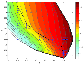
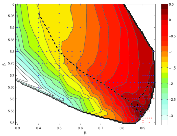
Figure 3: Left: Landscape of the baryonic density. Right: Landscape of the baryon density susceptibility. The color scale (right) is based on $\log_{10}(n_{B})$.

The algorithm works reasonably well over a large range of parameters even at small temperature. The model permits to vary $\mu$, $\kappa$, $\beta$ as independent parameters and it is reasonably cheap to measure various correlations. In fig. 3 we show the “landscape” of the real part of the baryon density $n_{B}$ (while the imaginary part is compatible with zero inside the statistical errors). The main variation is an exponential growth with $\mu$ indicating that we do not see yet saturation effects. This masks to a certain extent the finer structure. A clearer view of the situation is provided by looking at the “landscape” of the susceptibility of the baryon density (fig 3). A ridge is clearly visible, highlighted by a dashed black line. A second line (dashed) is explained later. We found it therefore advantageous to look at the Polyakov loops and their susceptibility. In fig. 4 we show the Polyakov loop susceptibility vs. $\beta$ at fixed $\mu$ and on the bottom vs. $\mu$ at fixed $\beta$ and, in fig 5 (right) the corresponding landscape. The plots of the Polyakov loop susceptibility show quite clearly maxima indicating possible transitions or crossovers. In the landscape fig. 5, one of these maxima shows up as a well defined ridge, indicated by a dashed black line. It shows only a moderate slop in $\mu$, which explains why the maxima are more pronounced when we vary $\beta$ at fixed $\mu$ than vice versa.

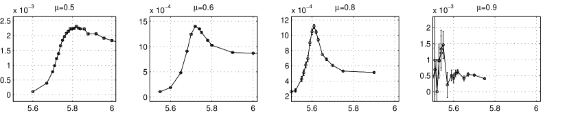
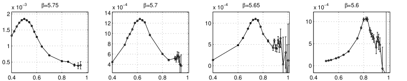
Figure 4: Polyakov loop susceptibility vs. $\beta$ at fixed $\mu$ (top) and vs. $\mu$ at fixed $\beta$ (bottom).

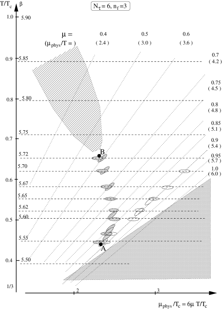
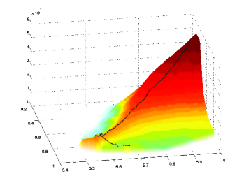
Figure 5: Left: the phase diagram in the $\beta$ (or $T/T_{c}$) - $\mu_{phys}/T_{c}$ QCD plane. The dotted straight lines correspond to constant $\mu$, the dashed ones to constant $\beta$. Right: landscape of the Polyakov loop susceptibility (top) and its 3d view (bottom). The color scale is based on $\log_{10}(\chi_{P})$.

The broadening of this ridge at small $\mu$ as well as of the maximum in Fig. 4 is responsible for the loss of a sharp transition signal at small $\mu$. These figures clearly show that the transition at fixed $\mu=0.50$ is less steep than the one at $\mu=0.80$. Presumably at $\mu<\sim 0.6$ we are dealing with a crossover, whereas at large $\mu$ the signal is more compatible with a real phase transition. Notice that changing $\beta$ at fixed $\mu$, we cross the transition line at a more oblique angle at smaller $\mu$, but the broadening of the ridge and loss of a transition signal is a genuine effect, as can be seen from fig. 5. A second ridge branching off from this main ridge at large $\mu$, highlighted by a dotted line is suggested by looking at the level lines in fig. 5 and corresponds to the second maximum suggested at large $\mu$ in fig. 4. This may indicate the appearance of the new phase at large $\mu$ and small $T/T_{c}$ discussed above.

We used the results for the Polyakov loop susceptibility to estimate the possible position of the transition points in the $\beta$ vs. $\mu$ plane (see [8] for details); to go half way toward a possible physical interpretation the positions determined in this way are indicated by the blobs in the diagram $T/T_{c}$ vs. $\mu_{phys}/T_{c}$ of fig. 5, where $\mu_{phys}=\mu/a(\beta)=N_{\tau}\mu T$. The shaded blobs correspond to the rather unambiguous ‘deconfining’ signal observed for $\mu>\sim 0.6$ ($\beta<\sim 5.72$). The ‘transition’ line suggested by this signal starts at the lower point A on the figure, located at $\beta\simeq 5.55,\,\mu\simeq 0.88$, i.e., with our rough estimation $\mu_{phys}/T_{c}\simeq 2.4,\,T/T_{c}\simeq 0.45$ (below which we could no longer obtain reliable data) and ends at the point B located near $\beta\simeq 5.72,\,\mu\simeq 0.6$, i.e., with our rough estimation $\mu_{phys}/T_{c}\simeq 2.3,\,T/T_{c}\simeq 0.65$. Above this point the signal becomes ambiguous.

The picture emerging from the data is thus the following: for $\mu<0.5-0.6$ ($\mu_{phys}/T\sim 3$) there is only a broad crossover, while for $0.6<\mu<0.9$ ($3.6<\mu_{phys}/T<5.3$) there is evidence of a sharper crossover or transition at a value $\mu_{c}$ depending on $\beta$. Moreover, for $\mu\simeq 0.9$ there is some evidence of the presence of the second transition even though this evidence is much weaker than the other one because at larger values of $\mu$ the fermion determinant strongly oscillates and, indeed, the usual sign problem manifest its effects.

To summarize our results, the phase structure found by the numerical simulations for $n_{f}=3$ is shown in fig. 5. The signal for the deconfining transition (or narrow crossover) on the line connecting A and B is rather good and it also appears that at small $\mu$ (above B) the transition is smoothed out in accordance with the expectations from full QCD simulations [1, 9]. A second transition at large $\mu$ could only be identified tentatively. In this region, the diquark susceptibility grows strongly [8]. This region needs further study to reach a conclusion, but it is interesting that the general picture shows qualitative agreement with the one found in the mean field approximation.

We can consider this model as an evolved ‘quenched approximation’ in the presence of charged matter. Then this study would give us information about the modified gluon dynamics of the SU(3) theory in this situation. It would then be natural to think of it as providing a heavy, dense, charged background for propagation of light quarks and calculate light hadron spectra and other hadronic properties under such conditions. This could also help fixing a scale controlling the behavior of the light matter. Work in progress goes in this direction.

References

- [1] F. Karsch, J. Phys. Conf. Ser. 46 (2006) 122 [hep-lat/0608003]; Nucl. Phys. A783 (2007) 13 [hep-ph/0610024].
- [2] I. Bender, T. Hashimoto, F. Karsch, V. Linke, A. Nakamura, M. Plewnia, I.-O. Stamatescu, W. Wetzel, Nucl. Phys. Proc. Suppl. 26 (1992) 323.
- [3] J. Engels, O. Kaczmarek, F. Karsch, E. Laermann, Nucl. Phys. B558 (1999) 307 [hep-lat/9903030].
- [4] T. C. Blum, J. E. Hetrick and D. Toussaint, Phys. Rev. Lett. 76 (1996) 1019 [hep-lat/9509002]; O. Kaczmarek, Ph.D. Thesis, Bielefeld 2000; A. Yamaguchi, Nucl. Phys. Proc. Suppl. 106 (2002) 465.
- [5] G. Aarts O. Kaczmarek, F. Karsch, I.-O. Stamatescu, Nucl. Phys. Proc.Suppl. 106 (2002) 456 [hep-lat/0110145].
- [6] R. Hofmann and I.-O. Stamatescu, Nucl. Phys. Proc. Suppl. 129 (2004) 623 [hep-lat/0309179].
- [7] R. De Pietri, A. Feo, I.-O. Stamatescu, E. Seiler, PoS LAT2005 (2006) 170 [hep-lat/0509167].
- [8] R. De Pietri, A. Feo, E. Seiler, I.-O. Stamatescu, arXiv:0705.3420 [hep-lat], to appear in Phys. Rev. D.
- [9] Y. Aoki, Z. Fodor, S. D. Katz and K. K. Szabo, Phys. Lett. B643 (2006) 46 [hep-lat/0609068].