Pair correlations in sandpile model: a check of logarithmic conformal field theory

Abstract

We compute the correlations of two height variables in the two-dimensional Abelian sandpile model. We extend the known result for two minimal heights to the case when one of the heights is bigger than one. We find that the most dominant correlation $\log r/r^{4}$ exactly fits the prediction obtained within the logarithmic conformal approach.

Conformal field theory has proved to be extraordinarily powerful in the description of universality classes of equilibrium critical models in two dimensions cft . Critical exponents, correlation functions, finite-size scaling, perturbations and boundary conditions, among others, have all been studied within the conformal approach, and thoroughly (and successfully) compared with numerical data.

More recently, increased interest has been turned toward logarithmic conformal theories, as a larger class of conformal theories, interesting in its own right, but also as a description of certain non-equilibrium lattice models. In particular, dense polymers polym ; log , sandpile models sand ; jpr and percolation perc ; log are lattice realizations of logarithmic conformal theories. An infinite series of such lattice models have been defined in log .

The logarithmic theories are however much lesser understood than the more usual, non-logarithmic ones. This is due to their higher level of complexity, which somehow reflect the complexity of the associated lattice models. Indeed the models mentioned above all have intrinsic non-local features. In this respect, it may appear to be strange, if not miraculous, that a lattice model with non-local variables can be described, in the scaling limit, by a local field theory. The only trace the lattice non-localities leave in the continuum local theory seems to be the presence of logarithms in correlation functions.

It is therefore essential to check that the logarithmic conformal description is indeed appropriate for these models, as extensively as it has been done for equilibrium critical phenomena (see for instance henkel ).

It is our purpose in this Letter to take further steps in this necessary procedure, in the context of the two-dimensional Abelian sandpile model. A certain number of checks have been carried out for this model (see sand ), but the one we propose here is more crucial because it deals with microscopic variables which are manisfestly non-local, and for which the logarithmic conformal theory makes a very definite prediction. It therefore exposes in the clearest possible way the non-local features of the model.

Namely, we compute, in the infinite discrete plane, the 2-site correlations $P_{1i}(r)-P_{1}P_{i}$ of two height variables, one of which being equal to 1, the other, $h_{i}$, being equal to 2, 3 or 4 (here $P_{i}$ is the 1-site probability on the infinite plane). Conformal field theory predicts that the dominant term of these is given by jpr

$$P_{1i}(r)-P_{1}P_{i}=c_{i}{\log r\over r^{4}}+\ldots,$$ (1)

with known coefficients $c_{i}$. New and explicit lattice calculations, to be detailed below, fully confirm these results, and exactly reproduces the coefficients $c_{i}$.

Logarithmic conformal theory also predicts that the 2-site correlations $P_{ij}(r)-P_{i}P_{j}$ of two heights bigger or equal to 2 decay like ${\log^{2}r/r^{4}}$, but the explicit lattice calculation of these remains out of range for the moment.

I The sandpile model and logarithmic conformal theory

We briefly recall the sandpile model introduced by Bak, Tang and Wiesenfeld in btw (see ipd for further details).

Every site $i$ of a finite rectangular grid $\mathcal{L}$ is assigned a height variable $h_{i}$, taking the four values $1,2,3$ and 4. A configuration $\mathcal{C}$ is the set of values $\{h_{i}\}$ for all sites. A discrete stochastic dynamics is defined on the set of configurations. If $\mathcal{C}_{t}$ is the configuration at time $t$, the height at a random site $i$ of $\mathcal{C}_{t}$ is incremented by 1, $h_{i}\to h_{i}+1$, making a new configuration $\mathcal{C}^{\prime}_{t}$. If the (new) height $h_{i}$ in $\mathcal{C}^{\prime}_{t}$ is smaller or equal to 4, one simply sets $\mathcal{C}_{t+1}=\mathcal{C}^{\prime}_{t}$. If not, all sites $j$ such that their height variables $h_{j}$ exceed 4 topple, a process by which $h_{j}$ is decreased by 4, and the height of all the nearest neighbours of $j$ are increased by 1. That is, when the site $j$ topples, the heights are updated according to

$$h_{i}\to h_{i}-\Delta_{ji},$$ (2)

with $\Delta$ the discrete Laplacian, $\Delta_{ii}=4$, $\Delta_{ij}=-1$ for nearest neighbour sites, and $\Delta_{ij}=0$ otherwise. This toppling process stops when all height variables are between 1 and 4; the configuration so obtained defines $\mathcal{C}_{t+1}$.

The boundary sites are dissipative, because a toppling there evacuates one or two grains of sand, which we imagine are collected in a sink site, connected to all dissipative sites. The presence of dissipative sites is essential for the dynamics to be well-defined, since it makes sure that the toppling process stops in a finite time.

When the dynamics is run over long periods, the sandpile builds up, being subjected to avalanches spanning large portions of the system. This correlates the height variables over very large distances, and makes the system critical in the thermodynamic limit.

It turns out that, when the dynamics is run for long enough, and no matter what the initial configuration is, the sandpile enters a stationary regime, in which only special configurations occur with equal probability, the so-called recurrent configurations ddhar . The recurrent set ${\cal R}$ forms a small fraction of all configurations, since

$$|{\cal R}|=\det\Delta\simeq(3.21)^{N},$$ (3)

where $N$ is the number of sites. So the asymptotic state of the sandpile is controlled by a unique invariant distribution $P_{\mathcal{L}}^{*}$, uniform on the set ${\cal R}$ of recurrent configurations, and zero on the non-recurrent (transient) ones. In the infinite volume limit, the invariant measure $P^{*}_{\mathcal{L}}$ is believed to become a conformal field theoretic measure.

To be recurrent, the height values of a configuration must satisfy certain global conditions ddhar , leading to non-local features. For what follows, it will be enough to know that the recurrent configurations are in one-to-one correspondence with oriented spanning trees on $\mathcal{L}^{\star}$, the original lattice $\mathcal{L}$ supplemented with the sink site. This change of variables, more convenient to perform actual calculations, also yields a different lighting on the non-localities of the model.

Spanning trees are acyclic configurations of arrows: at each site $i$ of $\mathcal{L}$, there is an outgoing arrow, pointing to any one of its $\Delta_{ii}$ neighbours (if $i$ is dissipative, the arrow can point to the sink site). A configuration of arrows defines a spanning tree if it contains no loop. By construction, the paths formed by the arrows all lead to the sink site $\star$, which is the root of the tree.

The mapping between recurrent configurations and trees is complicated and non-local; however the spanning trees provide an equivalent description. The global conditions that the heights of recurrent configurations have to satisfy are encoded in the property of arrow configurations of containing no loop, also a global constraint. The invariant measure $P^{*}_{\mathcal{L}}$ becomes simply a uniform distribution on the spanning trees.

Height values at a given site can be related to properties of spanning trees. To do so, one defines the notion of predecessor: a site $j$ is a predecessor of $i$ if the unique path from $j$ to the root passes through $i$. Then it has been shown Priez that the trees in which the site $i$ (not on the boundary) has exactly $a-1$ predecessors among its nearest neighbours correspond to configurations where $h_{i}\geq a$, for $a=1,2,3$ or 4. So configurations with $h_{i}=1$ are associated with trees which have a leaf at $i$; this is a local property which may be verified by looking at the neighbourhood of $i$ only. In contrast, heights 2, 3 and 4 correspond to non-local properties in terms of the trees.

Using this correspondence, joint probabilities for heights $P[h_{i}=a,h_{j}=b,\ldots]$ can be related to the fractions of trees satisfying certain conditions regarding the number of predecessors of $i,j,\ldots$ among their nearest neighbours. However, because of the remark we have just made, probabilities with heights 1 only are considerably easier than those involving higher heights. So far, the only probabilities involving higher heights in the bulk which have been computed are the 1-site probabilities $P[h_{i}=a]$ on the upper-half plane jpr . They provided enough input to assess the conformal nature of the four height variables in the scaling limit.

The logarithmic conformal theory, relevant to the sandpile model, has central charge $c=-2$. Among the distinctive features of a logarithmic theory is the presence of reducible yet indecomposable Virasoro representations; this property in turn introduces logarithms in their correlators lcft .

The fields describing the scaling limit of the four lattice height variables $\delta(h_{z}-i)-P_{i}$, which we call $h_{i}(z)$, have been determined in jpr . As hinted by the remarks made above, the height 1 field is very different from the other heights’ fields. It turns out that $h_{1}$ is a primary field with conformal weights $(1,1)$, while the other three, $h_{2},h_{3}$ and $h_{4}$, are all related to a single field, identified with the logarithmic partner of $h_{1}$. More precisely, if $h_{1}$ is the primary field normalized as the height 1 variable on the lattice, then $h_{2}$ satisfies the triangular relations,

$$L_{0}h_{2}=h_{2}-{1\over 2}h_{1},\quad L_{1}h_{2}=\rho,\quad L_{-1}\rho=-{1\over 4}h_{1},$$ (4)

where $\rho$ is a (0,1) field. In fact, $h_{1}$ and $h_{2}$ are members of the non-chiral version of the indecomposable representation called ${\cal R}_{2,1}$ in gk2 . The last two fields are linear combinations, $h_{3}=\alpha_{3}h_{2}+\beta_{3}h_{1}$, $h_{4}=\alpha_{4}h_{2}+\beta_{4}h_{1}$, and may also be viewed as logarithmic partners of $h_{1}$. The coefficients $\alpha_{i},\beta_{i}$ are such that $h_{3}$ and $h_{4}$, like $h_{1}$ and $h_{2}$, have the same normalization as their lattice counterparts; their exact values are known jpr .

The identification of the height fields makes it possible to compute correlations. In particular the joint probabilities for two height variables on the infinite plane $\mathbb{Z}^{2}$ correspond, in the scaling limit, to 3-point correlators in the conformal theory,

$$P_{ij}(z_{1},z_{2})-P_{i}P_{j}=\langle h_{i}(z_{1})h_{j}(z_{2})\omega(\infty)\rangle,$$ (5)

where $\omega$ is a weight (0,0) conformal field, logarithmic partner of the identity jpr . Indeed the infinite plane should be thought of as the limit of a growing finite grid, which has dissipation located along the boundary. In the infinite volume limit, the boundaries, and with them, the dissipation, are sent off to infinity. The field $\omega$ precisely realizes the insertion of dissipation at infinity, required for the sandpile model to be well-defined.

The 3-point correlators have been computed in jpr , and take the general form ($z_{12}\equiv z_{1}-z_{2}$)

$$\langle h_{i}(z_{1})h_{j}(z_{2})\omega(\infty)\rangle={A_{ij}+B_{ij}\log|z_{12}|+C_{ij}\log^{2}|z_{12}|\over|z_{12}|^{4}},$$ (6)

where $C_{ij}=0$ if $\min(i,j)=1$, and moreover $B_{11}=0$ and $A_{11}=-P_{1}^{2}/2$ Dhar , so that, depending on $i$ and $j$, one, two or three terms in the numerator are present. The coefficient of the dominant term, i.e. the largest power of $\log|z_{12}|$, could be determined exactly, and yields the dominant contribution of the 2-site probabilities jpr

$$P_{1i}(r)-P_{1}P_{i} \simeq -{\alpha_{i}P_{1}^{2}\over 2r^{4}}\log r,\qquad i>1,$$ (7)

$$P_{ij}(r)-P_{i}P_{j} \simeq -{\alpha_{i}\alpha_{j}P_{1}^{2}\over 2r^{4}}\log^{2}r,\qquad i,j>1,$$ (8)

where $P_{1}=2(\pi-2)/\pi^{3}$, as first computed in Dhar , and

$$\alpha_{2}=1,\quad\alpha_{3}={8-\pi\over 2(\pi-2)},\quad\alpha_{4}=-{\pi+4\over 2(\pi-2)}.$$ (9)

II Calculations on the lattice

It has been shown in Dhar and Priez (see also jpr for details) that height probabilities $P_{i}$ in the ASM can be reduced to the computation of determinants of discrete Laplacian matrices perturbed by a number of defects. The resulting matrices $\Delta^{\prime}=\Delta+B$ differ from the regular Laplacian by a defect matrix $B$, with $B=0$ except for a finite number of elements. Given a lattice point $t_{0}$, non-zero elements of $B$ related to $t_{0}$ can be marked by arrows at adjacent bonds (Fig.1).

Figure 1: Non-zero elements of $B$ related to $t_{0}$ (arrowed bonds) for (a) $\Delta^{\prime}=\Delta+B_{1}$, (b) $\Delta^{\prime}=\Delta_{\text{local}}$ and (c) $\Delta^{\prime}=\Delta_{\text{loop}}$. The bond $[t_{0},t_{4}]$ in $\Delta_{\text{loop}}$ is weighted by $-\varepsilon$.

For instance, the non-zero part of the matrix $B=B_{1}$ used for the evaluation of $P_{1}$ (Fig.1a) is

$$B_{1}={\small\left(\begin{array}[]{ccccc}-3&1&1&1\\ 1&-1&0&0\\ 1&0&-1&0\\ 1&0&0&-1\\ \end{array}\right)},$$ (10)

where rows and columns are labeled by $t_{0}$, $t_{2}$, $t_{3}$, $t_{4}$. The probability to have a height $1$ at $t_{0}$ is then Dhar

$$P_{1}=\frac{\det(\Delta+B_{1})}{\det\Delta}=\det({\mathbb{I}}+B_{1}G),$$ (11)

where $G=\Delta^{-1}$. The explicit form of the translation invariant Green function on the plane, $G(\vec{r})\equiv G_{\vec{r},\vec{0}}=G_{0,0}+g_{p,q}$ for $\vec{r}=(p,q)$,

$$g_{p,q}=\frac{1}{8\pi^{2}}\int\!\!\!\!\int_{-\pi}^{\pi}\frac{e^{ip\alpha}e^{iq\beta}-1}{2-\cos\alpha-\cos\beta}{\rm d}\alpha{\rm d}\beta,$$ (12)

implies $P_{1}=2(\pi-2)/\pi^{3}$.

The probability to have a height $2$ can be written Priez as

$$P_{2} = P_{1}+\frac{4\det\Delta_{\text{local}}}{\det\Delta}+\lim_{\varepsilon\to\infty}\frac{4\det\Delta_{\text{loop}}}{\varepsilon\det\Delta}+$$ (13)

$$+ \sum_{[a,b,c]}\lim_{\varepsilon\to\infty}\frac{2\det\Delta_{\Theta}}{\varepsilon^{3}\det\Delta},$$

where the defect matrices related to $\Delta_{\text{local}}$ and $\Delta_{\text{loop}}$ are shown in Fig.1b-c, and that related to $\Delta_{\Theta}$ is on the left side of Fig.2. The matrix $\Delta_{\Theta}$ differs from $\Delta$ by the removed bond $[j_{0},j_{3}]$ and three additional matrix elements (bonds) weighted by $-\varepsilon$ between the sites $j_{0}$, $j_{2}$, $j_{4}$ and a triplet of neighbouring sites $[a,b,c]$, whose position and orientation (see Fig.3) are to be summed over the whole lattice, with the restriction that the group $[a,b,c]$ does not overlap with $j_{0}$, $j_{2}$, $j_{3}$, $j_{4}$.

Figure 2: Structure of matrix $\Delta_{1\Theta}$. On the left side, the defects are the removed bond $[j_{3},j_{0}]$ and three additional bonds $[j_{4},b]$, $[j_{0},c]$, $[j_{2},a]$ with weight $-\varepsilon$. The right part shows the same defect as in Fig.1a.

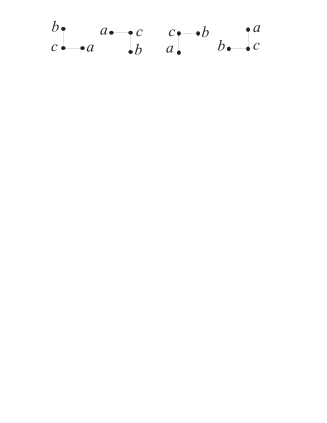
Figure 3: Four possible orientations of the group $[a,b,c]$.

The 2-site probability $P_{12}$ combines the defect of $\Delta_{1}$ with those of $\Delta_{\text{local}}$, $\Delta_{\text{loop}}$ and $\Delta_{\Theta}$. Simple calculations show that the matrices $\Delta_{\text{local}}$ and $\Delta_{\text{loop}}$ contribute a term $1/r^{4}$ to the asymptotics of $P_{12}(r)$ for large $r$, and are therefore subdominant. Thus the leading contribution comes from the matrix $\Delta_{1\Theta}$ combining the defects of $\Delta_{1}$ and $\Delta_{\Theta}$, as shown in Fig.2. The correlation function $P_{1\Theta}(r)$ is

$$P_{1\Theta}(r)={\sum_{[a,b,c]}}^{\prime}\lim_{\varepsilon\to\infty}\frac{2\det\Delta_{1\Theta}}{\varepsilon^{3}\det\Delta},$$ (14)

where the prime means that the sum excludes the terms where at least one edge in the group $[a,b,c]$ overlaps a deleted edge adjacent to $t_{0}$. The ten forbidden positions are shown in Fig.4.

Figure 4: Forbidden positions of the group [a,b,c].

The ratios of determinants in Eq.(14) are computed as $\det({\mathbb{I}}+B_{1\Theta}G)$, like Eq.(11), where the non-zero part of $B_{1\Theta}=\Delta_{1\Theta}-\Delta$ is a $8\times 9$ block diagonal matrix. The first block is

$$B_{\Theta}={\small\left(\begin{array}[]{ccccc}1&-1&0&0&0\\ 0&0&-\varepsilon&0&0\\ 0&0&0&-\varepsilon&0\\ 0&0&0&0&-\varepsilon\\ \end{array}\right)},$$ (15)

with rows $j_{3},j_{0},j_{2},j_{4}$ and columns $j_{0},j_{3},c,a,b$, while the second block is $B_{1}$ in Eq.(10). For large $r\gg 1$, we can replace all Green functions containing $r$ by their asymptotic value,

$$g_{p,q}=-\frac{\ln(p^{2}+q^{2})}{4\pi}-\frac{1}{\pi}\left(\frac{\gamma}{2}+\frac{3}{4}\log 2\right),$$ (16)

where $p^{2}+q^{2}\gg 1$ and $\gamma=0.57721\ldots$ is the Euler constant. Expanding the determinants in Eq.(14), we obtain, for the sum over the forbidden positions,

$$F(r)=\frac{2(\pi-2)^{2}}{\pi^{6}}\frac{\log r}{r^{4}}+O\left(\frac{1}{r^{4}}\right).$$ (17)

We can now write the desired correlation in the form

$$P_{1\Theta}(r)-P_{1}P_{\Theta}=2\left(\sum_{\vec{s}}\mathcal{U}_{r}(\vec{s})-F(r)\right),$$ (18)

where the sum is taken over all lattice points $\vec{s}=(k,l)$ and $P_{\Theta}$ is the last term in Eq.(13). The function $\mathcal{U}_{r}(\vec{s})$ behaves as $r^{-4}$, if $s>r\gg 1$ and as $s^{-4}r^{-4}\log r$, if $r\gg 1$, $s\gg 1$, $s<r$. In the region $r\gg 1$ and $s<r$, we have

$$\mathcal{U}_{r}(\vec{s})=Q_{k,l}\frac{\log r}{r^{4}}+O\left(\frac{1}{r^{4}}\right),$$ (19)

where we find, after some algebra,

$$Q_{k,l} = \frac{(\pi-2)^{2}}{4\pi^{6}}\Bigl{(}g_{k-1,l-1}-4g_{k-1,l}+g_{k-1,l+1}$$ (20)

$$- g_{k,l-2}+4g_{k,l}-g_{k,l+2}-g_{k+1,l-1}$$

$$+ 4g_{k+1,l}-g_{k+1,l+1}-2g_{k+2,l}\Bigr{)}.$$

The summation over all $k$, $l$ yields

$$\sum_{k=-\infty}^{+\infty}\sum_{l=-\infty}^{+\infty}Q_{k,l}=\frac{(\pi-2)^{2}}{\pi^{6}}.$$ (21)

Finally, we obtain

$$P_{1\Theta}(r)-P_{1}P_{\Theta}=-\frac{2(\pi-2)^{2}}{\pi^{6}}\frac{\log r}{r^{4}}+O\left(\frac{1}{r^{4}}\right),$$ (22)

which coincides with the LCFT prediction (7) for $i=2$. Similar calculations for $P_{13}(r)$ and $P_{14}(r)$ fully confirms the results (7) with the correct values of the coefficients.

Despite a very specific form of $\Delta_{\Theta}$, the correlation functions $P_{1i}(r)$, $i=2,3,4,$ are the first example where the logarithmic corrections to pair correlations can be computed explicitly.

References

- (1) P. Di Francesco, P. Mathieu and D. Sénéchal, Conformal Field Theory, Springer Verlag, New York 1996.
- (2) H. Saleur, Nucl. Phys. B 382, 486 (1992); E.V. Ivashkevich, J. Phys. A 32, 1691 (1999); P.A. Pearce and J. Rasmussen, J. Stat. Mech. P02015 (2007).
- (3) P.A. Pearce, J. Rasmussen and J.-B. Zuber, J. Stat. Mech. P11017 (2006); N. Read and H. Saleur, Nucl. Phys. B 777, 316 (2007).
- (4) S. Mahieu and P. Ruelle, Phys. Rev. E 64, 066130 (2001); P. Ruelle, Phys. Lett. B 539, 172 (2002); M. Jeng, Phys. Rev. E 69, 051302 (2004); G. Piroux and P. Ruelle, J. Stat Mech. P10005 (2004); M. Jeng, Phys. Rev. E 71, 036153 (2005); E 71, 016140 (2005); G. Piroux and P. Ruelle, J. Phys. A: Math. Gen. 38, 1451 (2005); S. Moghimi-Araghi, M.A. Rajabpour and S. Rouhani, Nucl. Phys. B 718, 362 (2005).
- (5) G. Piroux and P.Ruelle, Phys. Lett. B 607, 188 (2005); M. Jeng, G. Piroux and P. Ruelle, J. Stat. Mech. P10015 (2006).
- (6) M.A. Flohr and A. Müller-Lohmann, J. Stat. Mech. P12006 (2005); P04002 (2006); P.A. Pearce and J. Rasmussen, J. Stat. Mech. P09002 (2007); P. Mathieu and D. Ridout, arXiv:0707.0802.
- (7) M. Henkel, Conformal Invariance and Critical Phenomena, Springer Verlag, New York 1999.
- (8) P. Bak, C. Tang and K. Wiesenfeld, Phys. Rev. Lett. 59, 381 (1987).
- (9) E.V. Ivashkevich and V.B. Priezzhev, Physica A 254, 97 (1994); D. Dhar, Physica A 369, 29 (2006).
- (10) D. Dhar, Phys. Rev. Lett. 64, 1613 (1990).
- (11) V.B.Priezzhev, J. Stat. Phys 74, 955 (1994).
- (12) V. Gurarie, Nucl. Phys. B 410, 535 (1993); M.A. Flohr, Int. J. Mod. Phys. A 18, 4497 (2003); M.R. Gaberdiel, Int. J. Mod. Phys. A 18, 4593 (2003).
- (13) M. R. Gaberdiel and H. G. Kausch, Nucl. Phys. B 477, 293 (1996); M. R. Gaberdiel and H. G. Kausch, Nucl. Phys. B 538, 631 (1999).
- (14) S.N. Majumdar and D. Dhar, J. Phys. A: Math. Gen. 24 L357-L362 (1991).