Theoretical progress on $\pi\pi$ scattering lengths and phases

Abstract:

$\pi\pi$ scattering at low energy is sensitive to the structure of the QCD vacuum. I review the calculations of the $\pi\pi$ scattering lengths and phases, and group them in three cathegories: 1. those based on very general theoretical constraints (like dispersion relations and crossing symmetry) and phenomenology, 2. those which in addition make explicit use of chiral symmetry, 3. the first-principle ones, done with lattice QCD. I then compare these to the experimental results. Thanks to recent progress in all these and in the experimental determination of the scattering lengths we are improving substantially our knowledge of the QCD vacuum.

1 Introduction

According to the standard view, the pions become massless in the chiral limit, because they play the role of the Goldstone bosons of spontaneous chiral symmetry breaking. The strength of the interaction among Goldstone bosons vanishes with the square of their momentum and with a calculable coefficient (the inverse of the decay constant squared). If one moves away from the chiral limit, the strength of the interaction does not vanish when they are at rest, but for small quark masses it must be proportional to them. The coefficient of this term is also calculable and is given by the quark condensate (divided by the decay constant to the fourth power). These few statements summarize what was known about $\pi\pi$ scattering already more than 40 years ago, when Weinberg calculated the amplitude using current algebra [1]:

$$A(s,t,u)=\frac{s-M^{2}}{F^{2}}+\mathcal{O}(p^{4})\;\;,$$ (1)

where $A(s,t,u)\equiv\mathcal{M}(\pi^{+}\pi^{-}\to\pi^{0}\pi^{0})$ is the isospin invariant $\pi\pi$ scattering amplitude, $M^{2}\equiv B(m_{u}+m_{d})$, with $B=-\langle\bar{q}q\rangle/F^{2}$, is the leading term in the quark mass expansion of the pion mass squared, $M_{\pi}^{2}=M^{2}+\mathcal{O}(m_{q}^{2})$, and $F$ the pion decay constant in the chiral limit, $F_{\pi}=F+\mathcal{O}(m_{q})$. As indicated by the $\mathcal{O}(p^{4})$ symbol, the result of Weinberg is the leading term in the chiral expansion. Formula (1) clearly illustrate the importance of studying $\pi\pi$ scattering: Weinberg’s calculation heavily relies on a theoretical picture about the vacuum of QCD. The latter is difficult to rigorously prove theoretically (indeed, until we can prove it, this picture only has the status of a reasonable, sound assumption), and very difficult to test experimentally. In $\pi\pi$ scattering we are now able to do it.

This took quite some efforts, however, both on the theoretical and on the experimental side. On the theory side, one had to show that the beautiful relation between the scattering lengths, the quark masses, the quark condensate and the pion decay constant given by Eq. (1), valid at leading order of the chiral expansion, does not get washed out by higher order corrections. Not only a next-to-leading (NLO) [2], but also a NNLO calculation [3] were necessary to reach the required level of confidence. On the experimental side, for many years the only known reliable method to measure the $\pi\pi$ scattering lengths was through final state interactions in $K_{e4}$ decays [4]. It is worth stressing that this channel is quite rare (BR$\sim 10^{-5}$), and that the effect due to the $\pi\pi$ rescattering in the final state is rather subtle. The first measurement by the Geneva-Saclay collaboration [5] was based on about 30000 events, came only about ten years after Weinberg prediction (with which it disagreed!) and could only reach a precision of about 20% on the S-wave, isospin zero scattering length $a_{0}^{0}$. It took more than twenty years to see an improvement (by more than a factor of ten in the statistics) of that experiment, by the E865 collaboration at Brookhaven [6]. Today we are in the lucky situation of having not only yet another improvement in statistics by another experiment, NA48 (with the advantage of having also different systematics), but also two completely different ways to measure the $\pi\pi$ scattering lengths: the one pursued by DIRAC at CERN relies on the measurement of the lifetime of pionium, whereas the one pursued again by the NA48 Collaboration, also at CERN, on a very precise measurement of a small cusp in the spectrum of the center of mass energy of the two neutral pions in $K^{\pm}\to\pi^{\pm}\pi^{0}\pi^{0}$ decays.

A detailed knowledge of the $\pi\pi$ scattering amplitude is also important for many other hadronic processes, whenever pions in the final state play a role. Two examples of this are the determination of the $\sigma$ resonance parameters [7] (for a recent discussion of this issue and reference to the earlier literature see Ref. [8]), and the evaluation of the hadronic contributions to the $g-2$ of the muon [9].

Since a few years, there is a new player on the $\pi\pi$ scattering arena, lattice QCD. Various groups have calculated the isospin two, $S$ wave scattering length $a^{2}_{0}$ in the quenched approximation and the first calculations with dynamical fermions [10] and reasonably low quark masses have recently become available [11]. In addition, on the lattice one can explicitly see how both the pion mass and decay constant behave as one decreases the quark masses, and so directly test our picture of the QCD vacuum as one approaches the chiral limit. Using chiral perturbation theory (CHPT) one can translate this information into values of the scattering lengths and check whether all these informations merge into a coherent picture.

The rest of the paper is organized as follows: in the next section I will discuss dispersion relations and in particular the Roy equations and some phenomenological analyses based on them. These analyses rely on theory only as far as unitarity and analyticity (and partly crossing symmetry) are concerned, and use also data as input, but do not make any use of chiral symmetry. In the following section I will then discuss the improvement in precision which one obtains if one uses chiral symmetry. Section 4 gives an overview of the recent progress in related lattice calculations. I conclude and summarize in the final section.

2 Theoretical calculations which do not make use of chiral symmetry

In the early days of the study of strong interactions it was quickly realized that perturbative methods could not be applied. In order to tackle the problem in some more useful way, people tried to exploit the general properties of the $S$ matrix, like analyticity and unitarity and its possible symmetries. In $\pi\pi$ scattering this activity culminated in the formulation of an (infinite) set of coupled dispersion relations for all the partial waves, which incorporated analyticity and unitarity and (partially) crossing symmetry, by S. M. Roy [12]. The dispersion relations are double subtracted, and the two subtraction constants may be identified with the two $S$ wave scattering lengths, $a_{0}^{0}$ and $a^{2}_{0}$. Soon after the formulation of the equations different groups started to work on their numerical solution [13, 14] (and others on their mathematical properties, see e.g. [15], but we will not dwell on this point here). The outcome of these analyses was that at low energy the essential parameters are the two scattering lengths: given some reasonable input for the imaginary parts above a certain energy (called the matching point), the solution of the Roy equations uniquely fixes the partial waves below this energy in terms of the two scattering lengths. Notice that since at low energy only the $S$ and $P$ waves have imaginary parts significantly different from zero, the Roy equations can be solved effectively only for these, and become a set of three coupled integral equations. Of course the solutions do still depend on the input on the imaginary parts of the higher waves, but these are not particularly important and can be kept fixed (with the corresponding uncertainties properly taken into account). In such a setting if the uncertainty in the input would shrink to zero, the partial waves below the matching point would only depend on the two scattering lengths.

After about twenty years of inactivity in this field, in view of new experiments about $\pi\pi$ scattering, the study of the numerical solutions of Roy equations has been taken up again by a few groups [16, 17, 18, 19]. The results of the early analyses could be reproduced and the newly built machineries were ready to incorporate new experimental results. The logical flow of these analyses is as follows: take the input for the imaginary parts above the matching point with generous uncertainties. At this stage $a_{0}^{0}$ and $a_{0}^{2}$ are still completely free, apart from a loose correlation which takes the form of a rather wide band, called the universal band in the $(a_{0}^{0},a_{0}^{2})$ plane, see Fig. 1, left panel.

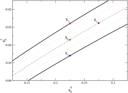
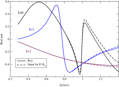
Figure 1: Left panel: universal band. Right panel: solution corresponding to the point $S_{0}$ at the center of the universal band. The matching point in this figure is $0.8$ GeV. Both figures are from Ref. [16].

If one knew exactly the input for the imaginary part of the exotic $S$ wave, one could not freely choose $a_{0}^{2}$: in order to have a smooth transition at the matching point, without unphysical cusps, $a_{0}^{2}$ has to be appropriately tuned. In this situation, the universal band would shrink to a line. Its width reflects the uncertainties in the experimental input for the exotic $S$ wave [20, 21] (for details about this point, cf. Ref. [16]). Unfortunately it is rather unlikely that we will see an improvement of this input – in the foreseeable future the universal band will stay as it is.

To any point inside the universal band there corresponds an exact solution of the Roy equations, as shown in Fig.1, right panel. Such a solution can be compared to any data set on the $\pi\pi$ scattering amplitude below the matching point. One can then vary the two scattering lengths and evaluate the $\chi^{2}$ corresponding to each point inside the universal band. The minimum of the $\chi^{2}$ identifies the value of the two scattering lengths that a certain data set prefers. Such an analysis has been done in the early days in Refs. [13, 14], and more recently repeated in Refs. [16, 17]. The latter two analyses agree as far as the solutions of the Roy equations are concerned – any difference in the conclusions arises from the use of different sets of data, but this is much less significant than the check provided by two completely independent analysis of the Roy equations.

This theoretical work is very important, but it is clear that by doing this one simply relates different data sets rather than making a genuine theoretical prediction: analyticity, unitarity and crossing symmetry do not fully constrain the $\pi\pi$ scattering amplitude at low energy, but imply that any measurement thereof can be translated into a measurement of the two $S$ wave scattering lengths, and this is what such an analysis concretely implements.

Kaminksi, Lesniak and Loiseau [18] have used the solution of the Roy equations in order to resolve an ambiguity in the extraction of the $\pi\pi$ scattering amplitude from $\pi N\to\pi\pi N$ data, and have so provided another example of how useful it is to take into account analyticity, unitarity and crossing symmetry in the data analysis. In this manner they have also obtained ranges for the scattering lengths, which we will compare to other analyses below.

A different approach has been followed by Peláez and Ynduráin [22]. They use a parametrization for each partial wave which is simple and respects analyticity in certain low energy regions, and fit data with these. They then check a posteriori whether forward dispersion relations are satisfied, and use this information to improve their fits. In a later work with Kaminski, [19] they have concentrated on the region above the $K\bar{K}$ threshold and reevaluated the dispersion relations. In comparison to other analyses, these works do not fully exploit analyticity and crossing symmetry. Moreover, there are some difference as far as the high-energy behaviour (described à la Regge) of the $\pi\pi$ scattering is concerned. The latter, however, has a limited influence in the low energy region (as shown in [23] in reply to the criticism raised in [24]). The main difference between this analysis and the other ones concerns the behaviour of the $S0$ wave in the region between $0.5$ GeV and the and $K\bar{K}$ threshold, where these authors claim that both data as well as dispersion relations would like to have a broad structure which they call a “shoulder”. As discussed by Leutwyler [25], this shoulder is in contrast with the Roy equations.

	no chiral symmetry			with chiral symm.
	DFGS [17]	KLL [18]	PY [22]	CGL [26]
$a_{0}^{0}$	$0.228\pm 0.032$	$0.224\pm 0.013$	$0.230\pm 0.015$	$0.220\pm 0.005$
$-10\cdot a_{0}^{2}$	$0.382\pm 0.038$	$0.343\pm 0.036$	$0.480\pm 0.046$	$0.444\pm 0.010$
$(\delta_{0}^{0}-\delta_{0}^{2})_{|}{{}_{s=M_{K}^{2}}}$	$47.1^{\circ}$	$37^{\circ}-\delta_{0}^{2}(M_{K}^{2})<49^{\circ}$	$52.9^{\circ}\pm 1.6^{\circ}$	$47.7^{\circ}\pm 1.5^{\circ}$

Table 1: Comparison of the numbers for the $S$-wave scattering lengths and the phase difference $\delta_{0}^{0}-\delta_{0}^{2}$ at $s=M_{K}^{2}$ for the theoretical analyses discussed here.

A comparison of the numbers for the $S$-wave scattering lengths and of the phase difference $\delta_{0}^{0}(M_{K}^{2})-\delta_{0}^{2}(M_{K}^{2})$ of the analyses just discussed is given in Table 1. The last column contains the result obtained when using chiral symmetry, which will be discussed in the next section. The main difference between the first three columns and the last one concerns the size of the error bars – chiral symmetry leads to a substantial increase of the precision. The analyses which do not make use of chiral symmetry agree among themselves as far as the central value of $a_{0}^{0}$ is concerned. The central values of $a_{0}^{2}$ show a larger scatter, which simply reflects the meagre experimental information about this quantity. Finally, the last row shows that the analysis of Peláez and Ynduráin has a higher $\delta_{0}^{0}$ phase around the $K$ mass. Direct extraction of the phase difference $\delta_{0}^{0}(M_{K}^{2})-\delta_{0}^{2}(M_{K}^{2})$ from $K\to 2\pi$ decays actually indicate an even larger value. After applying isospin breaking corrections, Cirigliano et al. [27] find $(\delta_{0}^{0}-\delta_{0}^{2})_{|}{{}_{s=M_{K}^{2}}}=(60.8\pm 4)^{\circ}$. The recent update of the measurement of $\Gamma(K_{S}\to\pi^{+}\pi^{-}(\gamma))/\Gamma(K_{S}\to\pi^{0}\pi^{0})$ by KLOE [28] pushes this number down by about three degrees. Notice that the isospin breaking correction is in this case very large, about $12^{\circ}$ [27] – its evaluation is far from straightforward, and despite the careful analysis of Cirigliano et al. the outcome is puzzling. Understanding the clash between the value extracted from $K\to 2\pi$ and all other experimental and theoretical analyses remains an open, very important problem.

In all these analyses, input on the $\pi\pi$ scattering amplitude at intermediate energies is essential. This is obtained from different experiments by also using some convenient parametrizations which incorporate at least partially the properties of analyticity and unitarity. Until some years ago this input came mostly from $\pi N\to\pi\pi N$ scattering experiments [30, 31, 32, 33]. More recently, production of two (or more) pions in hadronic decays of heavier states have also become important, in particular for what concerns the resonances in the region around $1$ GeV, like the $f_{0}(980)$, which has been studied in detail at BES [34] and at KLOE [35], see also [36, 37, 38].

3 Theoretical calculations which rely on chiral symmetry

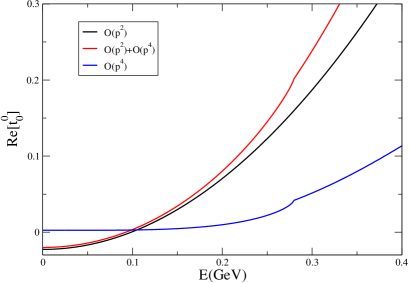
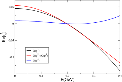
Figure 2: Behaviour of the $I=0$ (left panel) and $I=2$ $S$ waves in the region around threshold.

The Roy equations allow to translate any experimental information on $\pi\pi$ scattering at low energy into information on the scattering lengths. But one can also reverse the argument: if one has a theory which predicts the scattering lengths, one can combine this with the Roy equations and extend the prediction to the whole region below 1 GeV. As we have mentioned in the introduction, chiral symmetry does lead to predictions about the scattering lengths. The leading order calculation of Weinberg gives (after one substitutes $M^{2}$ and $F$ with $M_{\pi}^{2}$ and $F_{\pi}$, respectively)

$$a_{0}^{0}=\frac{7M_{\pi}^{2}}{32\pi F_{\pi}^{2}}=0.16\;,\qquad a_{0}^{2}=-\frac{M_{\pi}^{2}}{16\pi F_{\pi}^{2}}=-0.045\;\;.$$ (2)

The theoretical uncertainties of this prediction cannot be estimated until one evaluates the next term in the series. This was done by Gasser and Leutwyler in 1984 [2], and some ten years later even the correction one order higher has been evaluated [3]. Numerically the series behaves as follows:

$$a_{0}^{0}\stackrel{{\scriptstyle p^{2}}}{{=}}0.156\stackrel{{\scriptstyle p^{4}}}{{\to}}0.200\stackrel{{\scriptstyle p^{6}}}{{\to}}0.216\;,\qquad a_{0}^{2}\stackrel{{\scriptstyle p^{2}}}{{=}}-0.0454\stackrel{{\scriptstyle p^{4}}}{{\to}}-0.0445\stackrel{{\scriptstyle p^{6}}}{{\to}}-0.0445\;\;,$$ (3)

and shows a rather slow convergence in the $I=0$ channel. The reason for this slow convergence is understood and has to do with a rather hefty chiral log:

$$a_{0}^{0}=\frac{7M_{\pi}^{2}}{32\pi F_{\pi}^{2}}\left[1+\frac{9}{2}\ell_{\chi}+\ldots\right]\;,\qquad a_{0}^{2}=-\frac{M_{\pi}^{2}}{16\pi F_{\pi}^{2}}\left[1-\frac{3}{2}\ell_{\chi}+\ldots\right]$$ (4)

where $\ell_{\chi}=\frac{M_{\pi}^{2}}{16\pi^{2}F_{\pi}^{2}}\ln\frac{\mu^{2}}{M_{\pi}^{2}}$ which in turn is due to a strong rescattering of pions in this channel. The large corrections are unitarity effects, as it is also very well illustrated in Fig. 2: the correction of order $p^{4}$ shows a strong curvature below threshold and a sizeable cusp at threshold in the $I=0$ channel, but is very flat below and does not have a visible cusp at threshold in the $I=2$ channel. Around $s=0$, however, both corrections are very small.

This observation is crucial if one wants to combine the chiral prediction and the dispersive analysis: choosing the two scattering lengths as subtraction constants is convenient for discussing the physics, but it is not the only possible choice. One could as well subtract the amplitudes in the region below threshold. Doing this has the advantage that if one uses the chiral input there, this converges much better and gives stability to the whole machinery. Indeed, after subtracting below threshold, and evaluating the scattering lengths with the help of the Roy equations [26], the behaviour of the series improves drastically:

$$a_{0}^{0}\stackrel{{\scriptstyle p^{2}}}{{=}}0.197\stackrel{{\scriptstyle p^{4}}}{{\to}}0.2195\stackrel{{\scriptstyle p^{6}}}{{\to}}0.220\qquad a_{0}^{2}\stackrel{{\scriptstyle p^{2}}}{{=}}-0.0402\stackrel{{\scriptstyle p^{4}}}{{\to}}-0.0446\stackrel{{\scriptstyle p^{4}}}{{\to}}-0.0444\;\;.$$ (5)

Within this framework, the evaluation of the uncertainty can be done reliably, and gives

$$a_{0}^{0} = \;\;\,0.220\pm 0.001+0.027\Delta_{r^{2}}-0.0017\Delta\ell_{3}$$

$$10\cdot a_{0}^{2} = -0.444\pm 0.003-0.04\Delta_{r^{2}}-0.004\Delta\ell_{3}$$ (6)

where $\bar{\ell}_{3}=2.9+\Delta\ell_{3}$, is the low-energy constant which determines the next-to-leading quark mass dependence of the pion mass:

$$M_{\pi}^{2}=M^{2}\left(1-\frac{M^{2}}{32\pi^{2}F^{2}}\bar{\ell}_{3}+O(M^{4})\right)$$ (7)

and $\Delta_{r^{2}}$ is the relative uncertainty in the scalar radius of the pion, $\langle r^{2}\rangle_{s}=0.61\,\mathrm{fm}^{2}\cdot(1+\Delta_{r^{2}})$. The scalar radius strongly depends on the low energy constant $\bar{\ell}_{4}$, which determines the leading quark mass dependence of the pion decay constant:

$$F_{\pi}=F\left(1+\frac{M^{2}}{16\pi^{2}F^{2}}\bar{\ell}_{4}+O(M^{4})\right)\;.$$ (8)

Adding errors in quadrature and using the estimates $\Delta_{r^{2}}=6.5\%$ (which, together with the central value quoted above, corresponds to $\bar{\ell}_{4}=4.4\pm 0.2$), $\Delta\ell_{3}=2.4$ yields [26]

$$a_{0}^{0}=0.220\pm 0.005\;,\qquad a_{0}^{2}=-0.0444\pm 0.001\;,\qquad a_{0}^{0}-a_{0}^{2}=\;\;\,0.265\pm 0.004\;.$$ (9)

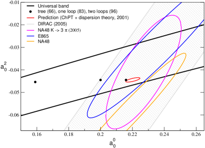
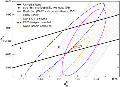
Figure 3: Comparison of the theoretical predictions of the scattering lengths and their measurements. On the left the blue and orange ellipses are obtained from the uncorrected $K_{e4}$ and on the right those after isospin corrections (cf. Ref. [40])

The experimental determinations of the scattering lengths have been amply discussed at this conference [39]. The comparison between the experimental numbers and the theoretical predictions is shown in Fig. 3. On the left panel the ellipses corresponding to the $K_{e4}$ data sets have been obtained with the raw data, whereas on the right panel the isospin breaking correction to the phase as extracted from $K_{e4}$ data, which has been evaluated and discussed in Ref. [40], has been applied. The figure shows that the latter isospin breaking correction is important at the current level of precision of the experiments. The disagreement at the level of 1.5 $\sigma$’s between the recent NA48 determination and the theoretical prediction disappears once this correction is taken into account. On the other hand, the perfect agreement seen on the left panel between the E865 determination and the theoretical prediction, becomes marginal, at the level of one sigma. In either case there is some tension between the E865 and the NA48 $K_{e4}$ data, which should be better understood This issue is discussed in detail in the contribution of Bloch-Devaux [39].

4 Lattice calculations

Lattice calculations relevant for $\pi\pi$ scattering can be grouped into two classes: those which determine the quark mass dependence of $M_{\pi}$ and $F_{\pi}$ and thereby determine the constants $\bar{\ell}_{3}$ and $\bar{\ell}_{4}$; and those which determine directly the scattering lengths. There are only two calculations of $a^{2}_{0}$ available until now with dynamical fermions, one of them is performed on a background containing only two dynamical quarks [10], while the more recent one by the NPLQCD collaboration is performed on a background of three flavours of staggered quarks [11] (on configurations generated by the MILC collaboration and made openly accessible). The latter calculation was done with a rather low pion mass, reaching values just below 300 MeV, such that an extrapolation down to physical pion masses becomes reliable. Their latest result reads

$$a_{0}^{2}=-0.04330\pm 0.00042$$ (10)

in excellent agreement with the chiral prediction (9), as it is also seen on Fig. 4. The CP-PACS calculation, on the other hand has been made for a value of the pion mass above 500 MeV, where contact with chiral perturbation theory, or an extrapolation to the physical value of the pion mass can hardly be possible. For the earlier literature on the subject, in particular on the quenched calculations, we refer the reader to Ref. [11].

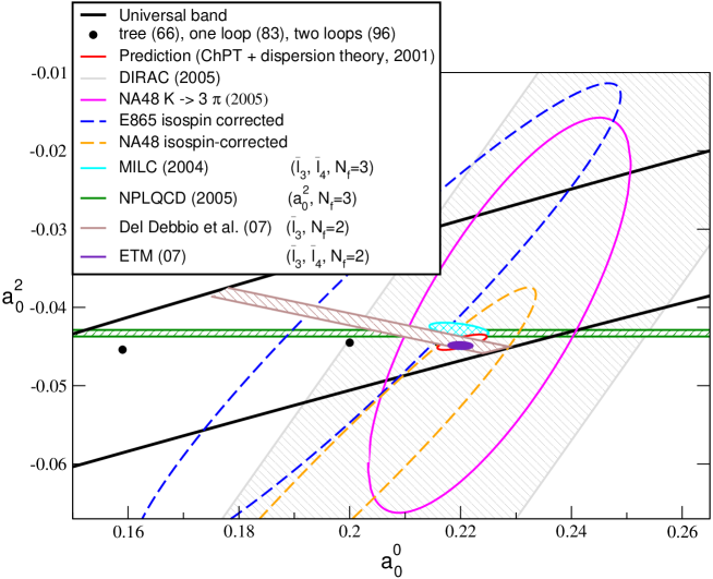
Figure 4: Same as Fig. 3, right panel, but including also lattice results.

The determination of the quark mass dependence of the pion mass and decay constant with dynamical fermions and for low pion masses has been performed by several groups. Published results are available from the MILC collaboration [41], from Del Debbio et al. [42] and from the ETM collaboration [43]. Only the first calculation has been done with a background of three dynamical flavours (of staggered quarks and employing the fourth root trick), whereas the last two have two light quarks in the sea (with a Wilson and twisted mass formulation, respectively). A summary of their numerical results is given in Table 2.

	MILC [41]	Del Debbio et al. [42]	ETM [43]
$\bar{\ell}_{3}$	$0.6\pm 1.2$	$3.5\pm 0.5\pm 0.1$	$3.65\pm 0.12$
$\bar{\ell}_{4}$	$3.9\pm 0.5$		$4.52\pm 0.06$

Table 2: Lattice determinations of the low energy constants $\bar{\ell}_{3}$ and $\bar{\ell}_{4}$.

The agreement with the phenomenological estimates is remarkable. It is important to stress the improvement in precision that the lattice approach offers for these constants, in particular for $\bar{\ell}_{3}$. In the long run the lattice method is without competition for this particular constant, and will compete with the phenomenological determination of others (notice that the errors given by the ETM collaboration do not include systematic effects – these have been estimated by the other two groups).

5 Summary and conclusions

The $\pi\pi$ scattering amplitude at low energy is one of the rare physical quantities that we can calculate with a high precision and that at the same time can be measured with a comparable precision. In addition, the comparison is very instructive, because we can relate the theoretical predictions made within the effective field theory framework to properties of the vacuum state of QCD. The recent progress in lattice calculations makes this issue even more interesting, because it allows us to compare experimental numbers directly to the result of first principle calculations, which only take as input the Lagrangian of QCD. All this is very well represented by Fig. 4, which shows (albeit in rather compressed form) the convergence of all these different informations. The figure also shows that we have room for improvement, especially on the experimental side, and possibly for surprises. It will be interesting to see how this picture will look like at the next Kaon conference.

References

- [1] S. Weinberg, Phys. Rev. Lett. 17 (1966) 616.
- [2] J. Gasser and H. Leutwyler, Annals Phys. 158 (1984) 142.
- [3] J. Bijnens, G. Colangelo, G. Ecker, J. Gasser and M. E. Sainio, Phys. Lett. B 374 (1996) 210 [arXiv:hep-ph/9511397].
- [4] N. Cabibbo and A. Maksymowicz, Phys. Rev. 137 (1965) B438
- [5] L. Rosselet et al., Phys. Rev. D 15 (1977) 574.
- [6] S. Pislak et al. [BNL-E865 Collaboration], Phys. Rev. Lett. 87 (2001) 221801 [arXiv:hep-ex/0106071].
- [7] I. Caprini, G. Colangelo and H. Leutwyler, Phys. Rev. Lett. 96 (2006) 132001 [arXiv:hep-ph/0512364].
- [8] M. R. Pennington, Mod. Phys. Lett. A 22 (2007) 1439 [arXiv:0705.3314 [hep-ph]].
- [9] G. Colangelo, Nucl. Phys. Proc. Suppl. 162 (2006) 256.
- [10] T. Yamazaki et al. [CP-PACS Collaboration], Phys. Rev. D 70 (2004) 074513 [arXiv:hep-lat/0402025].
-
[11]
S. R. Beane, P. F. Bedaque, K. Orginos and M. J. Savage [NPLQCD
Collaboration],
Phys. Rev. D 73 (2006) 054503
[arXiv:hep-lat/0506013];
S. R. Beane, T. C. Luu, K. Orginos, A. Parreno, M. J. Savage, A. Torok and A. Walker-Loud, arXiv:0706.3026 [hep-lat]. - [12] S. M. Roy, Phys. Lett. B 36 (1971) 353.
- [13] M. R. Pennington and S. D. Protopopescu, Phys. Rev. D 7 (1973) 1429.
- [14] J. L. Basdevant, C. D. Froggatt and J. L. Petersen, Nucl. Phys. B 72 (1974) 413.
-
[15]
T. P. Pool,
Nuovo Cim. A45 (1978) 207.
L. Epele and G. Wanders, Nucl. Phys. B 137 (1978) 521.
J. Gasser and G. Wanders, Eur. Phys. J. C 10 (1999) 159 [arXiv:hep-ph/9903443]. - [16] B. Ananthanarayan, G. Colangelo, J. Gasser and H. Leutwyler, Phys. Rept. 353 (2001) 207 [arXiv:hep-ph/0005297].
- [17] S. Descotes-Genon, N. H. Fuchs, L. Girlanda and J. Stern, Eur. Phys. J. C 24 (2002) 469 [arXiv:hep-ph/0112088].
- [18] R. Kaminski, L. Lesniak and B. Loiseau, Phys. Lett. B 551 (2003) 241 [arXiv:hep-ph/0210334].
- [19] R. Kaminski, J. R. Pelaez and F. J. Yndurain, Phys. Rev. D 74 (2006) 014001 [Erratum-ibid. D 74 (2006) 079903] [arXiv:hep-ph/0603170].
- [20] M. J. Losty et al., Nucl. Phys. B69 (1974) 185.
- [21] W. Hoogland et al., Nucl. Phys. B126 (1977) 109.
- [22] J. R. Pelaez and F. J. Yndurain, Phys. Rev. D 71 (2005) 074016 [arXiv:hep-ph/0411334].
- [23] I. Caprini, G. Colangelo, J. Gasser and H. Leutwyler, Phys. Rev. D 68 (2003) 074006 [arXiv:hep-ph/0306122].
- [24] J. R. Pelaez and F. J. Yndurain, Phys. Rev. D 68 (2003) 074005 [arXiv:hep-ph/0304067].
- [25] H. Leutwyler, AIP Conf. Proc. 892 (2007) 58 [arXiv:hep-ph/0612111].
- [26] G. Colangelo, J. Gasser and H. Leutwyler, Nucl. Phys. B 603 (2001) 125 [arXiv:hep-ph/0103088].
- [27] V. Cirigliano, G. Ecker, H. Neufeld and A. Pich, Eur. Phys. J. C 33 (2004) 369 [arXiv:hep-ph/0310351].
- [28] F. Ambrosino et al. [KLOE Collaboration], Eur. Phys. J. C 48 (2006) 767 [arXiv:hep-ex/0601025].
- [29] F. J. Yndurain, R. Garcia-Martin and J. R. Pelaez, arXiv:hep-ph/0701025.
- [30] B. Hyams et al., Nucl. Phys. B64 (1973) 134.
- [31] S. D. Protopopescu et al., Phys. Rev. D7 (1973) 1279.
- [32] G. Grayer et al., Nucl.Phys. B75 (1974) 189.
- [33] P. Estabrooks and A. D. Martin, Nucl. Phys. B79 (1974) 301.
- [34] M. Ablikim et al. [BES Collaboration], Phys. Lett. B 607 (2005) 243. [arXiv:hep-ex/0411001].
- [35] F. Ambrosino et al. [KLOE Collaboration], Eur. Phys. J. C 49 (2007) 473 [arXiv:hep-ex/0609009].
- [36] N. N. Achasov and A. V. Kiselev, Phys. Rev. D 73 (2006) 054029 [Erratum-ibid. D 74 (2006) 059902] [arXiv:hep-ph/0512047].
- [37] G. Isidori, L. Maiani, M. Nicolaci and S. Pacetti, JHEP 0605 (2006) 049 [arXiv:hep-ph/0603241].
- [38] D. V. Bugg, Eur. Phys. J. C 47 (2006) 45 [arXiv:hep-ex/0603023].
- [39] B. Bloch-Devaux, these proceedings. L. Di Lella, these proceedings. L. Tauscher, these proceedings.
- [40] J. Gasser, these proceedings, arXiv:0710.3048 [hep-ph].
-
[41]
C. Aubin et al. [MILC Collaboration],
Phys. Rev. D 70 (2004) 114501
[arXiv:hep-lat/0407028];
C. Bernard et al., arXiv:hep-lat/0611024. - [42] L. Del Debbio, L. Giusti, M. Luscher, R. Petronzio and N. Tantalo, JHEP 0702 (2007) 056 [arXiv:hep-lat/0610059].
- [43] Ph. Boucaud et al. [ETM Collaboration], Phys. Lett. B 650 (2007) 304 [arXiv:hep-lat/0701012].