Urban traffic from the perspective of dual graph

Abstract

In this paper, urban traffic is modeled using dual graph representation of urban transportation network where roads are mapped to nodes and intersections are mapped to links. The proposed model considers both the navigation of vehicles on the network and the motion of vehicles along roads. The road’s capacity and the vehicle-turning ability at intersections are naturally incorporated in the model. The overall capacity of the system can be quantified by a phase transition from free flow to congestion. Simulation results show that the system’s capacity depends greatly on the topology of transportation networks. In general, a well-planned grid can hold more vehicles and its overall capacity is much larger than that of a growing scale-free network.

I Introduction

Traffic problem is of great importance for the safety and convenience of modern society NS ; Helbing ; Kerner ; BML ; CKH ; Angel . The traffic research was mainly focused on the highway traffic NS ; Helbing ; Kerner or the traffic on a well-planned grid lattice BML ; CKH ; Angel . Recently, empirical evidences have shown that many transportation systems can be described by complex networks characterized by the small world WS and/or scale-free properties BA . The prototypes include urban road network BJiang ; Rosvall ; Crucitti ; Crucitti2 ; Porta , nation-wide road network Kala , public transport network Sien ; LiP , railway network Sen ; LiKP , airline transport systems LiW , and so on. And due to the importance of large communication networks such as the Internet and WWW, much investigation have been focused on ensuring free traffic flow and avoiding traffic congestion on networks.

In urban traffic, one natural approach is the “primal” representation which considers intersections as nodes and road segments as links between nodes. However, this representation can not characterize the common notion of “main roads” in urban traffic systems. Moreover, it violates the intuitive notion that an intersection is where two roads cross, not where four roads begin, so that it can not represent the way we usually tell each other how to navigate the road network Kala , e.g., “stay in Manning Road ignoring 4 crossings, until you reach the Kent Street and turn right.”

Here, we study the urban traffic by employing the dual representation of the road network, in which a node represents a single road, and two nodes are linked if their corresponding roads intersect. This kind of transformation was firstly proposed in the field of urban planning and design with the name Space Syntax Hiller ; Hiller2 ; Penn , and has been used recently to study the topological properties of urban roads BJiang ; Rosvall ; Crucitti ; Crucitti2 ; Porta . In this dual presentation, the “main roads” of the city can be represented by the “hub nodes” in the network. The node degree is not limited and it was found that the dual degree distribution of some cities follows a power-law.

One shortcoming of the dual representation is the abandonment of metric distance so that a street is one node no matter how long it is. However, the metric distance is the core of most traffic flow studies. To avoid this problem, this paper propose a traffic flow model considering the movement of vehicles along the road. We show that by using two parameters characterizing the road and intersection capacity, it is possible to simulate the urban traffic and seek out the overall capacity of the urban transportation system.

II Dual Graph of Urban Network and the Traffic Model

The basic steps of dual representation can be explained as following: one should firstly define which road segments belong together. Previous studies grouped the segments by line of sight by a driver Hiller ; Hiller2 ; Penn , their street name BJiang ; Rosvall , or by using a threshold on the angle of incidence of segments at an intersection Crucitti ; Crucitti2 ; Porta . Then, in the derived “dual graph” or the “connectivity graph”, each road is turned into one node, while each intersection is turned into one link.

II.1 Characterize Dual Graph Considering Traffic Problem

With this new paradigm, one can look at urban traffic problem from a new perspective. From common sense, the “main roads” can usually be characterized by long length, wide road width, many intersections, and high traffic efficiency. When the main roads are congested, the entire transportation system will be in danger of capacity drop. While the system will remain high efficiency even when some minor roads are jam.

In dual network, the major roads in urban system can be represented with hub nodes with many links, large capacity, and more handling ability. In particular, when considering the traffic flow problem, the characteristics of nodes can be introduced in the dual graph of urban network:

(1) Degree $k_{i}$ and degree distribution: The degree (or connectivity) of node $i$ is the number of links connecting to that node. In the dual graph of urban network, the degree corresponds to the number of intersections along road $i$. Thus there is no limit of node degree and so the “main roads” can be represented by the “hub nodes” in the system.

The way the degree is distributed among the nodes can be investigated by calculating the degree distribution $P(k)$, i.e., the probability of finding nodes with $k$ links. Networks with a power-law distribution are called scale-free BA .

(2) Capacity $C_{i}$: The capacity of road $i$ is the maximum number of vehicles the road can hold. This value can be calculated by: $C_{i}=L_{i}/l_{v}$, where $L_{i}$ is the length of the road, and $l_{v}$ is the vehicle’s average length. In the simulation, we assume that the length of each road segment are same, thus $C_{i}$ is proportional to the degree of the node: $C_{i}=\alpha\times k_{i}$, where $\alpha$ denotes the maximum number of vehicles that one road segment can hold. The system’s total capacity is the sum of the capacity of all node, that is $C_{t}=\Sigma_{i}C_{i}$.

(3) Turning Ability $T_{i}$: The turning ability is the maximum number of vehicles turning from the road to neighboring roads per time step. This value reflects the capacity of intersections along the road, and can be also measured in real practice. In the dual representation of urban traffic, $T_{i}$ is the maximum number of vehicles a node can send to neighboring nodes. Without losing generality, we assumed that all intersections can handle the same number of vehicle-turning from each road, thus $T_{i}$ is also proportional to the degree of the node: $T=\beta\times k_{i}$, where $\beta$ denotes the ability of one intersection.

II.2 Traffic Model

In dual network, the trajectory of a vehicle can be interpreted as traveling along some roads (nodes) for some distance, and jumping from a node to another node through an link representing an intersection. The proposed traffic model considers both the navigation of vehicles in the network and the movement of vehicles along roads. The model is partially motivated by the vehicular traffic models NS ; Helbing ; Kerner and by the traffic models of packet flow on the Internet Sole ; Arenas ; Tadic ; Zhao ; Wang . On the base of underlying dual infrastructure (discussed in Section III and IV), the system evolves in parallel according to the following rules:

1. Add Vehicles - At each time step, vehicles are added to the system with a given rate $R$ at randomly selected nodes and each new vehicle is given a random destination node.

2. Navigate Vehicles - If a vehicle’s destination is found in its nearest neighborhood, its direction will be set to the target. Otherwise, its direction will be set to a neighbor $n$ with probability:

$$P_{n}={k^{\phi}_{n}\over\Sigma_{i}k^{\phi}_{i}},$$ (1)

where the sum runs over all neighbors, and $\phi$ is an adjustable parameter reflecting the driver’s preference with the roads. It is assumed that the vehicles use a local routing strategy: they are more ready to use a neighboring “main road” when $\phi>0$, and they are more likely to go to a minor road when $\phi<0$. Once a vehicle reach its destination, it will be removed from the system.

3. Vehicles Motion along Roads - The intersections along a road $i$ are numbered with serial integers from $1$ to $k_{i}$. We use these integers to reflect the sequence of intersections along the road. When a vehicle enters a road at the $mth$ intersection and leaves at the $nth$ intersection, it has to travel the distance of $d=l_{0}\times|m-n|$ along the road, where $l_{0}$ denotes the length of one road segment, and $|...|$ denotes taking the absolute value. For the velocity, we assumed that the traffic flow is homogeneous along one given road. In each time step, the mean velocity of vehicles on the road is calculated using the following equation:

$$v_{i}=V_{max}\times(1.0-\rho_{i}),$$ (2)

where $V_{max}$ is the maximum velocity in the urban system, and $\rho_{i}=N_{i}/L_{i}$ is the local vehicle density on that road. Equation (2) simply approximates that the vehicles will take $V_{max}$ when there is no vehicle on the road, and the velocity will decreases linearly until no vehicle can move when $\rho=1.0$. In each time step, the distance of each vehicle in the road will decrease by the amount of $v_{i}$ until $d=0$, i.e., it reaches the preferred exiting intersection.

4. Vehicle-Turning at Intersections - At each step, only at most $T_{i}$ vehicles can be sent from a node for the neighboring nodes. When the number of the vehicles at a selected node is full (see the introduction of $C_{i}$), the node won’t accept any more vehicles and the vehicle will wait for the next opportunity.

One can see that the core parameters characterizing the transportation system are $\alpha$, $\beta$ and $V_{max}$. And parameter $\phi$ characterizes the behavior of drivers. In the simulations, without losing generality, the road segment length $l_{0}$ is assumed to be $500$ meters, and the average vehicle length $l_{v}$ is $10$ meters. Thus we set $\alpha=50$, i.e., one road segment between two successive intersections can hold $50$ vehicles at most. The parameter $\beta$ is also set to be constant for all intersections, meaning that the vehicle-turning ability for each intersection in the system is the same. And each time step is assumed to represent $5$ seconds in reality. Thus if the maximum velocity is $20m/s$, the maximum velocity in Eq.2 will be $V_{max}=100$. With changing the values of $\beta$ and $V_{max}$, different ability of intersections and different road conditions can be simulated.

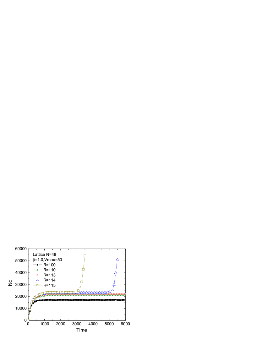
Figure 1: (Color online) Typical evolution of vehicle number in the grid system. The critical generating rate of vehicles is $R_{c}=113$.

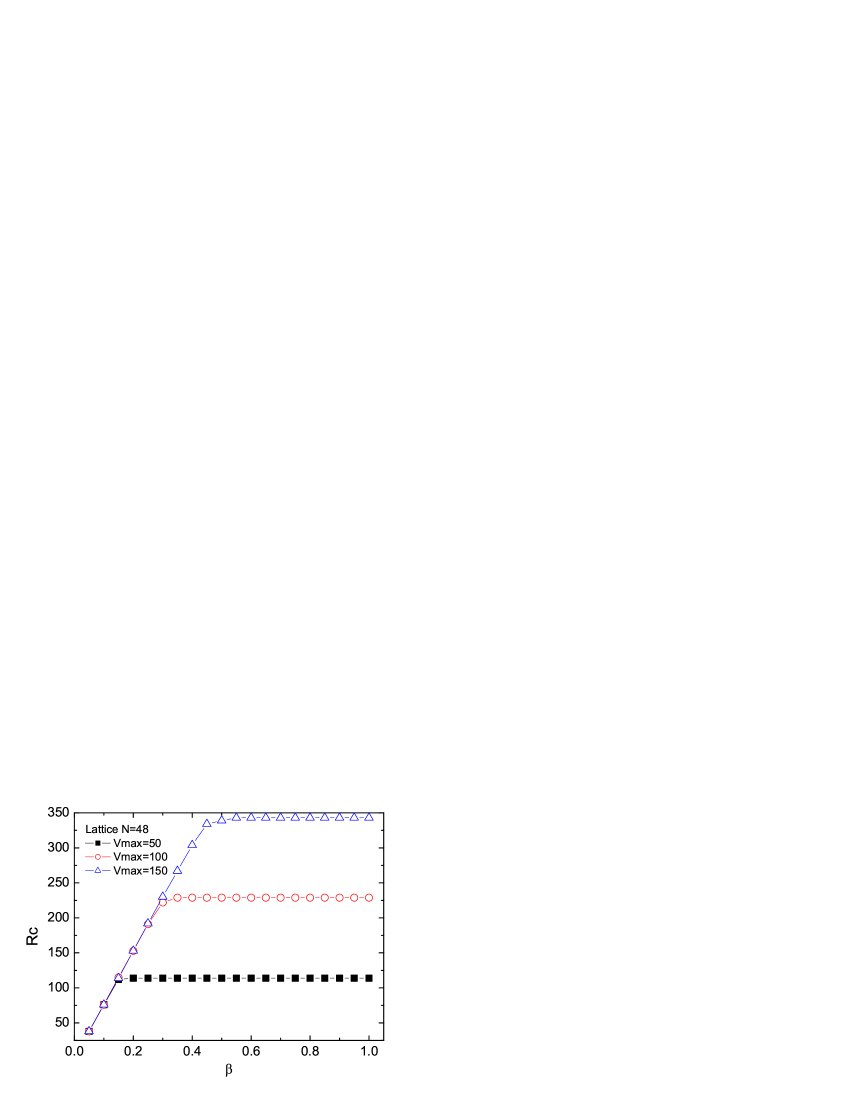
Figure 2: (Color online) $R_{c}$ vs $\beta$ with different values of $V_{max}$. The data are obtained by averaging $R_{c}$ with ten simulations.

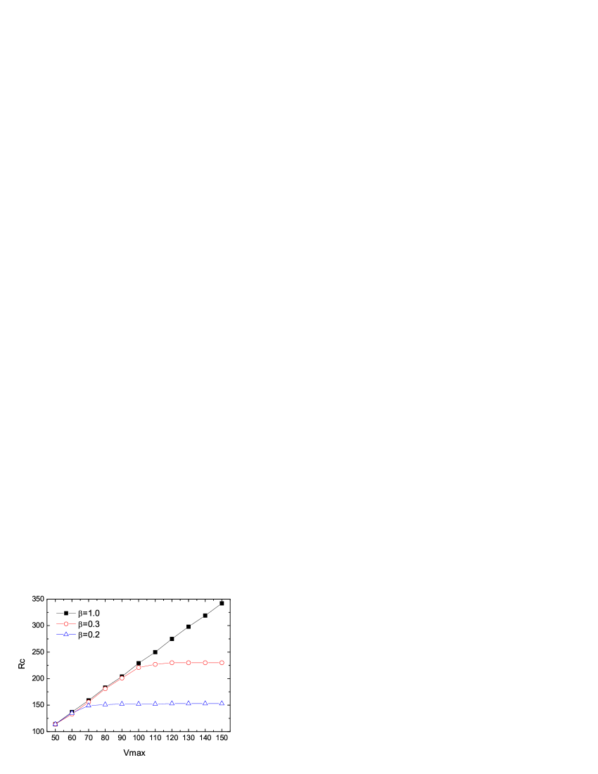
Figure 3: (Color online)$R_{c}$ vs $V_{max}$ with different values of $\beta$ . The data are obtained by averaging $R_{c}$ with ten simulations.

III Simulation of Urban Traffic on a Well-planned Lattice Network

In this section, the traffic on a well-planned grid urban network is simulated. The transportation network consists of 24 north-south roads crossing with 24 east-west roads. The studied system can be represented in dual graph by 48 nodes each with the same connectivity $k=24$. Thus there is no topological “main roads” in this system. For the case, $\phi=0$ is applied for all vehicles, i.e., they randomly select direction from neighboring roads if its destination is not found. Figure 1 displays the typical evolution of $N_{c}(t)$, i.e., the number of vehicles within the system for different generating rate R. One can see that when $R<R_{c}$, $N_{c}$ will increase first and then come to saturation, indicating the balance of the number of vehicles entering the system and the number of vehicles reaching their destinations. However, when $R>R_{c}$, $N_{c}$ can not remain constant. It will suddenly increase and quickly reach the the system’s total capacity. Thus the system is congested and the vehicles accumulate in the system. Therefore, the critical generating rate $R_{c}$ can be used to characterize the phase transition from free flow state to congestion. And the system’s overall traffic capacity can be measured by $R_{c}$ above which the system will enter the congested state.

To better understand the effects of intersection capacity and road condition on the overall efficiency, simulations with different values of $\beta$ and $V_{max}$ are carried out. Figure 2 shows the variance of overall capacity $R_{c}$ with $\beta$. One can see that $R_{c}$ firstly increases linearly with $\beta$ and then comes to saturation when $\beta$ is large enough. And the saturated value of $R_{c}$ increases with $V_{max}$. This result is in agreement with our common sense that we can not improve the overall efficiency only by enhancing intersection efficiency, but we should also enhance the road condition so that the vehicles can run faster on the road.

In Fig.3, one can see that $R_{c}$ increases with $V_{max}$ until a saturation is reached. Therefore, when the intersection capacity is large enough, the road condition will be a limitation for the whole system; while when the road condition is good enough, the intersection capacity will be crucial. Unfortunately, the vehicle speed can not be too large in the city. Thus there will be a unavoidable limit in improving urban traffic efficiency simply by enhancing intersection capacity, given that the network topology is fixed. One should think about other ways, such as adding shortcuts, developing subways, employing better navigation guidance system for the drivers, and so on.

IV Simulation of Urban Traffic on a Self-Organized Scale-Free Network

Recently, works on the centrality of roads in urban systems using dual representation Rosvall ; Sien ; Kala ; Crucitti ; Crucitti2 ; Porta show that the degree distribution of most planned cities is exponential, while it follows a power-law scaling in self-organized cities. That is, in most self-organized cities, there are some “main roads” with many minor roads intercrossing with them.

In this section, we try to simulate the urban traffic on a dual graph of scale-free network. To generate the underlying infrastructure, we adopt the well-known Barabási-Albert scale-free network model BA , in which the power-law distributions of degree is in good accordance with many real observations. In this model, starting from $m_{0}$ nodes fully connected by links with assigned weight $w_{0}$, the system are driven by two mechanics: (1) Growth: one node with $m$ links ($m\leq m_{0}$) is added to the system at each time step; (2) Preferential attachment: the probability $\Pi_{i}$ of being connected to the existing node $i$ is proportional to the degree $k_{i}$ of the node

$$\Pi_{i}={k_{i}\over\Sigma_{j}k_{j}},$$ (3)

where $j$ runs over all existing nodes.

As a remark, here we do not conclude that the BA network model exactly describes a self-organized system of urban roads. We adopt this model to reflect the fact that new roads are usually built to intercross with existing main roads. For example, the existing roads are often extended to new fields and branch roads are built from the extension of these roads. This mechanism can lead to the emergence of “main roads” in urban system, and it is quite similar to the “growth” and “preferential attachment” in BA model.

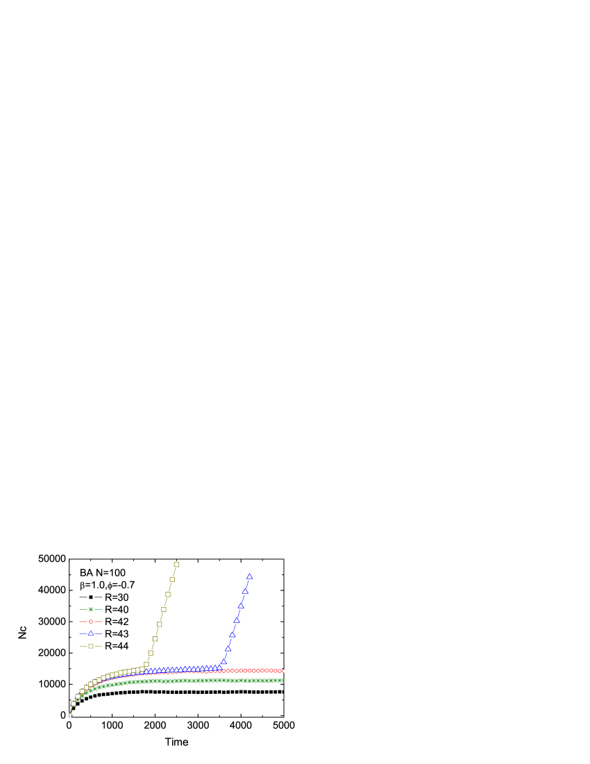
Figure 4: (Color online) Typical evolution of vehicle number in the scale-free system. The critical generating rate of vehicles is $R_{c}=42$.

Figure 4 shows the typical evolution of vehicle number in the system. The same behavior as in the lattice case can be observed. When $R<R_{c}$, the system is in free flow state, and the system will jam when $R>R_{c}$.

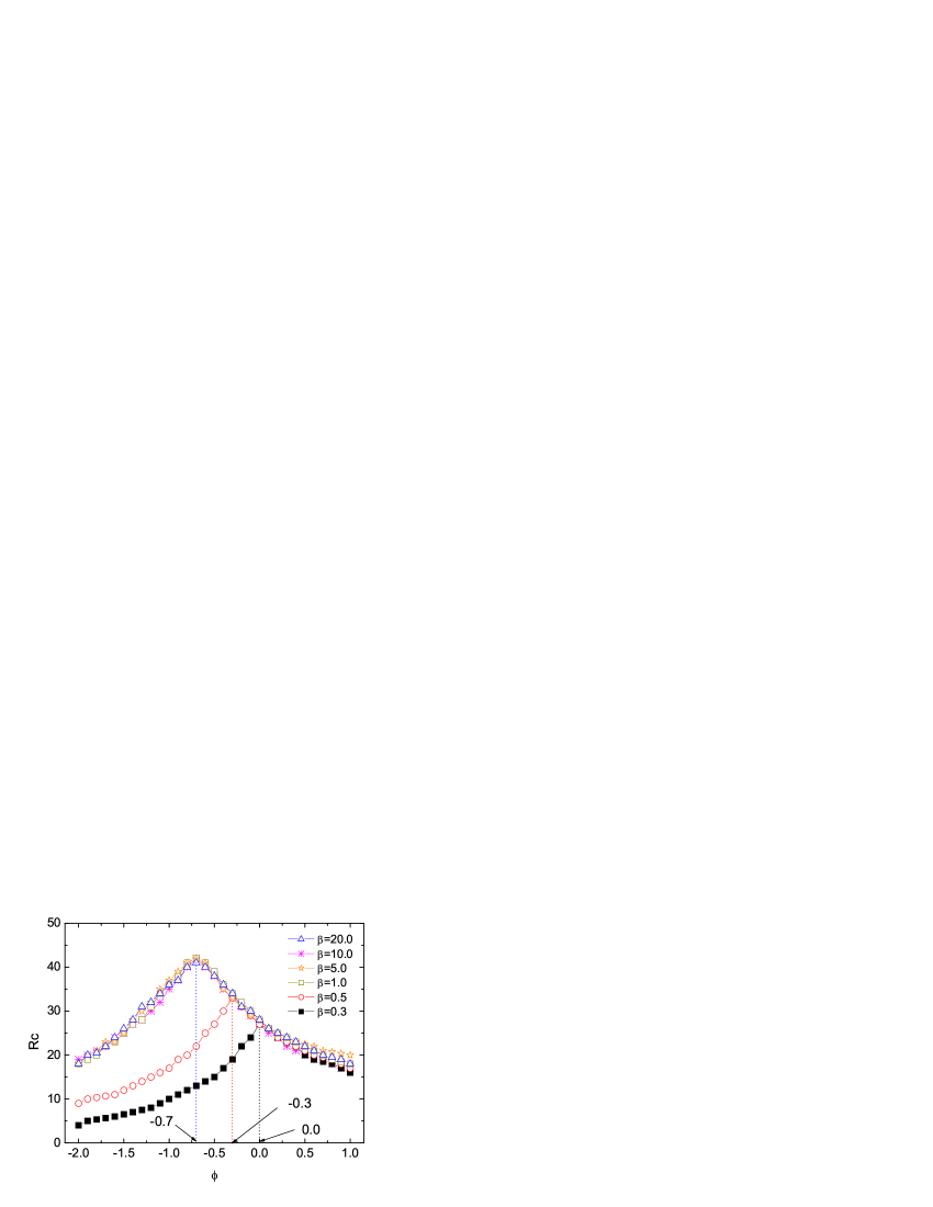
Figure 5: (Color online) The system’s capacity vs $\phi$ with $V_{max}=100$. The data are obtained by averaging $R_{c}$ over ten network realizations.

We first simulate the traffic on a network of $N=100$ nodes (roads) with $m_{0}=m=5$. This relatively small system can be seen as simulating the backbone of a city s urban traffic network. In such a scale-free network, it is very important to investigate the effect of navigation strategy on the overall capacity. Figure 5 depicts the variation of $R_{c}$ with $\phi$. It is shown that $R_{c}$ will be optimized at some typical value of $\phi_{c}$. For the case of $V_{max}=100$, when $\beta$ is above one, the system’s overall capacity will be optimized when $\phi_{c}=-0.7$ and with the $R_{c}\approx 42$. When $\beta$ decreases below one, the system’s efficiency will decrease rapidly. And the optimal value of $\phi$ will increase with the decrease of $\beta$. When $\beta=0.3$, $\phi_{c}=0.0$, implies that the best strategy is random-walk. We note that $\phi_{c}<0$ means to use the minor roads first. Therefore, if intersection capacity and road condition are the same for both main roads and minor roads, the best strategy for the whole system is to encourage drivers to use minor roads first.

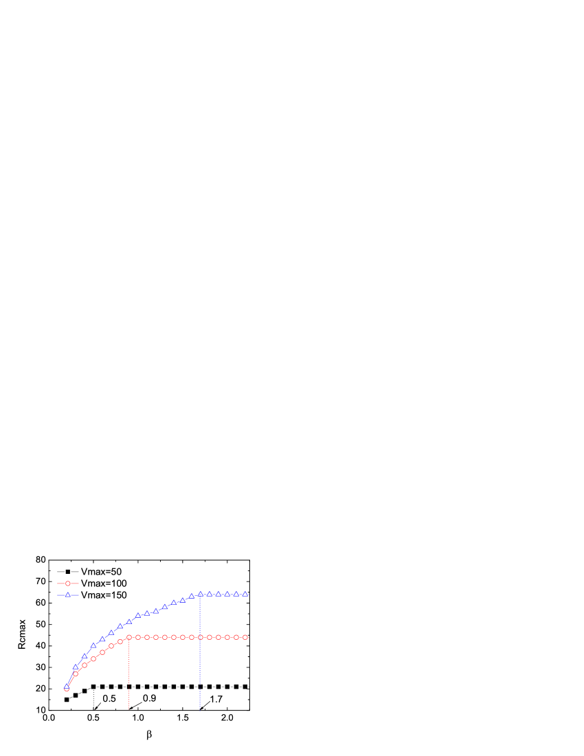
Figure 6: (Color online) The system’s maximal capacity $R_{cmax}$ vs $\beta$ with different $V_{max}$.

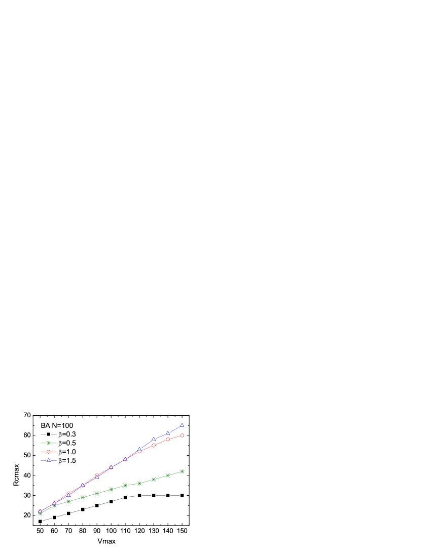
Figure 7: (Color online) The system’s maximal capacity $R_{cmax}$ vs $V_{max}$ with different $\beta$.

Figure 6 shows the variation of maximum value of $R_{c}$ (the peak value in Fig.5) with the increment of $\beta$ for different value of $V_{max}$. One can see that $R_{cmax}$ increase first and then come to saturation. And in Fig.7, the variation of $R_{cmax}$ with $V_{max}$ is shown. The behaviors are similar with the lattice grid case.

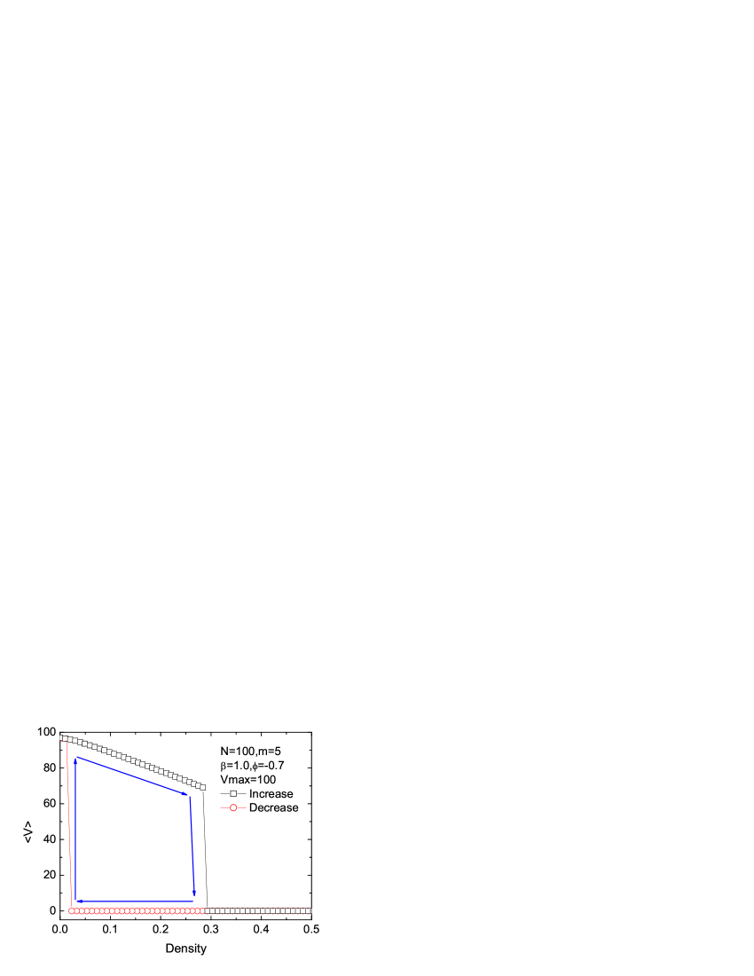
Figure 8: (Color online) Average velocity vs density. The black square line shows the velocity variation when adding vehicles to the system (increase density), while the red circle line shows the velocity variation when drawing out vehicles from the system (decrease density). The density values corresponding to the sudden transitions are 0.29 and 0.02 respectively. The arrows are showing the hysteresis as a guide for the eyes.

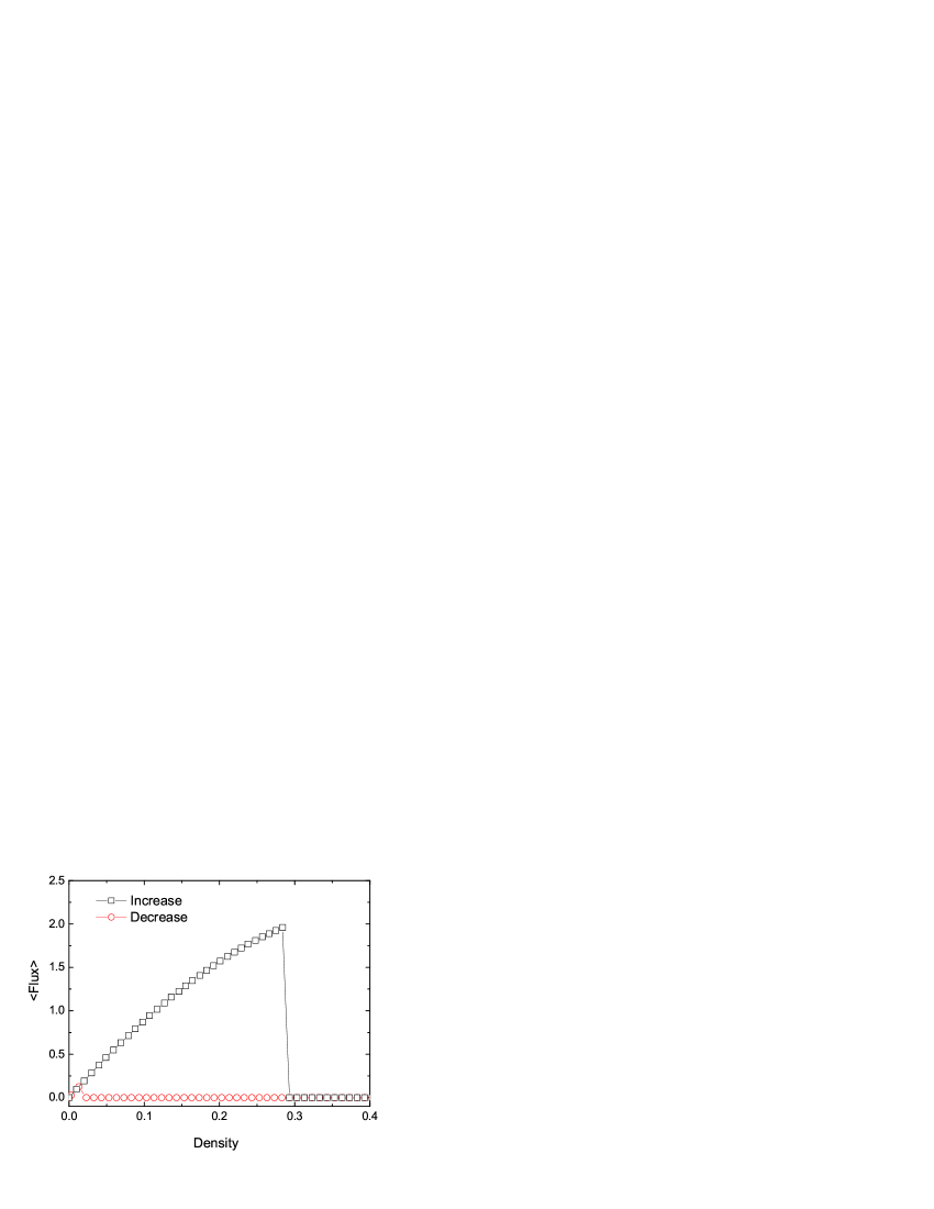
Figure 9: (Color online) Flux vs density.

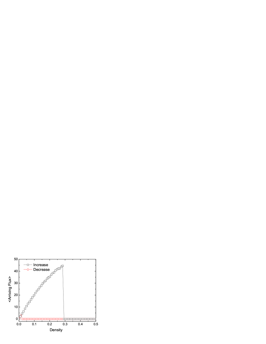
Figure 10: (Color online) Arriving flux vs density. Arriving flux vs density in the cases of increasing and decreasing density. Other parameters are the same as in Fig.8.

Finally, we try to reproduce the dependencies of average velocity and traffic flux on vehicle density, which are important criteria for evaluating the transit capacity of a traffic system. To simulate the case of constant vehicle density, the number of arrived vehicles at each time step is recorded, and the same number of vehicles are added to the system at the beginning of next step. In Fig.8, the velocity-density relation is displayed. Here the vehicle density of the system is calculated with $\rho=N_{c}/C_{t}$. The velocity firstly decreases gradually with the density. At the density of $0.29$, the velocity suddenly drops to zero, indicating the system enters the jam state. Two branches of the fundamental diagram coexist between $0.04$ and $0.29$. The upper branch is calculated by adding vehicles to the system (increasing density), while the lower branch is calculated by randomly removing vehicles from a jam state and allowing the system to relax after the intervention (decrease density). In this way a hysteresis loop can be traced (arrows in Fig.8). In the lower branch, the velocity keep zero until the density is very low. This is because some main roads are congested, thus the vehicles can not move on these roads, and this state will not be alleviated by removing vehicles randomly from the system.

Then we investigate the dependence of traffic flux on density. Two kinds of traffic flux are studied: the movement flux and the arriving flux. The movement flux is calculated as the product of average velocity and vehicle density. It corresponds to the average number of vehicles passing a given spot in the system per time step. Figure 9 shows this flux-density relation of the system. The arriving flux is calculated as the number of vehicles that successfully reach their destination in each time step. In Fig.10, the relation of arriving flux vs traffic density is shown. In both cases, the hysteresis exist between the same values of density as in Fig.8. And the maximum arriving flux (45 vehicles per step) is corresponding to $R_{c}=44$ when $V_{max}=100$ and $\beta=1.0$ as shown in Fig.6.

The system’s sudden drop to the jam state indicates a first-order phase transition. The phase transition and hysteresis can be explained as follows. According to the evolution rules, when a road is full of vehicles, the velocity will be zero and the vehicles on neighboring nodes can not turn to it. So the vehicles may also accumulate on the neighboring nodes and get congested. This mechanism can trigger an avalanche across the system when the density is high, thus a sudden phase transition happen at this point. As for the lower branch, starting from an initial congested configuration, the system will have some congested roads that are very difficult to dissipate. These roads will decrease the system efficiency by affecting the surrounding roads until all roads are not congested, thus we get the lower branch.

V Conclusions and Discussions

In conclusion, the urban traffic is simulated using a model based on dual approach. The model considers both the movement of vehicles on the road and the navigation of drivers in the system. The intersection and road conditions are naturally incorporated, and their effects on the whole system’s efficiency are investigated. In a systemic view of overall efficiency, the model reproduces several significant characteristics of urban traffic, such as phase transition, hysteresis, velocity-density relation and flux-density relation. The simulation results are a kind of similar to that of the BML model BML , which was proposed in 1992 to simulate the urban traffic on a square lattice. But the present model is more general, and with more interesting findings.

As comparing the simulation results on well-planned grid and on self-organized scale-free network, one can see that the grid network are more efficient than a self-organized one. Given that the total capacity ($C_{t}\approx 57,600$ and $50,000$) is almost the same for the two systems considered in this paper, the maximal number of vehicles running on the grid is more than that on the scale-free network (Fig.1 and 4), and the overall capacity $R_{c}$ takes much larger value on the lattice grid (Fig.2 and 6). This is in agreement with the previous studies showing that homogeneous networks can bear more traffic because of the absence of high-betweenness nodes Gui ; Tadic .

When considering the navigation on a scale-free network, the results are in agreement with previous studies that the traffic system will be more efficient by avoiding the central nodes Wang .

The work can be extended further in many ways. One can modify the model to capture more details in real traffic, such as the role of traffic lights, the differences between main roads and minor roads. Better navigation strategies can also be coined in the dual perspective. The resilience of traffic system against road failures will be of great importance and research interest.

References

- (1) K. Nagel, M. Schreckenberg, J. Phys. I France 2, 2221 (1992).
- (2) D. Helbing, B.A. Huberman, Nature (London) 396, 738 (1998).
- (3) B.S. Kerner, The Physics of Traffic, Springer, Berlin, NewYork (2004).
- (4) O. Biham, A.A. Middleton, D. Levine, Phys. Rev. A 46, R6124 (1992).
- (5) K.H. Chung, P.M. Hui, G.Q. Gu, Phys. Rev. E 51, 772 (1995).
- (6) O. Angel, A.E. Holroyd, J.B. Martin, Elec. Comm. in Prob. 10, 167 (2005).
- (7) D.J. Watts DJ, S.H. Strogatz, Nature (London) 393, 440 (1998).
- (8) R. Albert, H. Jeong, and A.-L. Barabási, Nature (London) 401, 130 (1999).
- (9) B. Jiang, C. Claramunt, Environ. Plan. B: Plan. Des. 31, 151 (2004).
- (10) M. Rosvall, A. Trusina, P. Minnhagen, K. Sneppen, Phys. Rev. Lett. 94, 028701 (2005).
- (11) P. Crucitti, V. Latora, S. Porta, Phys. Rev. E 73, 036125 (2006).
- (12) P. Crucitti, V. Latora, S. Porta, Chaos 16, 015113 (2006).
- (13) S. Porta, P. Crucitti, V. Latora, Physica A 369, 853 (2006).
- (14) V. Kalapala, V. Sanwalani, A. Clauset, C. Moore, Phys. Rev. E 73, 026130 (2006).
- (15) J. Sienkiewicz, J.A. Holyst, Phys. Rev. E 72(4), 046127 (2005).
- (16) P. Li, X. Xiong, Z.L. Qiao et al., Chin. Phys. Lett. 23(12), 3384 (2006).
- (17) P. Sen, S. Dasgupta, A. Chatterjee et al., Phys. Rev. E 67, 036106 (2003).
- (18) K.P. Li, Z.Y. Gao, B.H. Mao, Inter. J. Mod. Phys. C 17(9), 1339 (2006).
- (19) W. Li, X. Cai, Phys. Rev. E 69, 046106 (2004).
- (20) B. Hiller, J. Hanson, The Social Logic of Space, Cambridge University Press, Cambridge, UK (1984).
- (21) B. Hiller, Space is the Machine: A Configurational Theory of Architecture, Cambridge University Press, Cambridge, UK (1996)
- (22) A. Penn, B. Hillier, D. Banister, J. Xu, Enviro. Plan. B 25, 59 (1998).
- (23) R.V. Sole, S. Valverde, Physica A 289, 595 (2001).
- (24) A. Arenas, A. Díaz-Guilera, and R. Guimerá, Phys. Rev. Lett. 86, 3196 (2001).
- (25) B. Tadić, S. Thurner, G.J. Rodgers, Phys. Rev. E 69, 036102 (2004).
- (26) L. Zhao, Y.C. Lai, K. Park, N. Ye, Phys. Rev. E 71, 026125 (2005).
- (27) W.X. Wang, B.H. Wang, C.Y. Yin, Y.B. Xie, T. Zhou, Phys. Rev. E 73, 026111 (2006).
- (28) R. Guimerá, A. Díaz-Guilera, F. Vega-Redondo, A. Cabrales, A. Arenas, Phys. Rev. Lett. 89, 248701 (2002).
- (29) B. Tadić, G. J. Rodgers, and S. Thurner, e-print: arXiv:physics/0606166.