Moment Methods for Exotic Volatility Derivatives

Abstract.

The latest generation of volatility derivatives goes beyond variance and volatility swaps and probes our ability to price realized variance and sojourn times along bridges for the underlying stock price process. In this paper, we give an operator algebraic treatment of this problem based on Dyson expansions and moment methods and discuss applications to exotic volatility derivatives. The methods are quite flexible and allow for a specification of the underlying process which is semi-parametric or even non-parametric, including state-dependent local volatility, jumps, stochastic volatility and regime switching. We find that volatility derivatives are particularly well suited to be treated with moment methods, whereby one extrapolates the distribution of the relevant path functionals on the basis of a few moments. We consider a number of exotics such as variance knockouts, conditional corridor variance swaps, gamma swaps and variance swaptions and give valuation formulas in detail.

1. Introduction

Volatility derivatives are designed to facilitate the trading of volatility, thus allowing one to directly take a range of tailored views. A basic contract is the variance swap which upon expiry pays the difference between a standard historical estimate of daily return variance and a fixed rate determined at inception, see [D1992], [CM] and [DDKZ]. A variant on this is the corridor variance swap which differs from the standard variance swap only in that the underlying s price must be inside a specified corridor in order for its squared return to be included in the floating part of the variance swap payout [CL]. A further generalization is the conditional variance swap which pays the realized variance of an asset again within some corridor, whereby the average is taken only over the period when the spot is in the range. The advantage of conditional corridor variance swaps is that they allow one to take a view on volatility that is contingent upon the price level, gaining exposure to volatility only where required. Although conditional variance swaps appear to be traded, see  [JP], this is the first article in the open literature proposing a pricing methodology.

The numerical method we present extends without difficulties to other exotic volatility contracts such as variance swaptions, see also [CLee]. We also take the liberty of inventing exotic volatility derivatives such as variance knock-out options. These do not seem to be much traded although perhaps they should be. A variance knockout can be regarded as a variation on the theme of barrier knock-out options whereby the knock-out condition is not triggered by the underlying crossing a certain level. Instead, a variance knockout vanishes in case realized variance prior to maturity exceeds a certain pre-assigned threshold. The benefit of a variance knockout over a barrier knockout is that its hedge ratios are smoother.

In this paper, we use operator methods for pricing. Our presentation is self-contained for the specific purpose at hand but see the review article [A] for a more extended discussion of operator methods. One point we should stress is that the mathematical and numerical methods we present would work as efficiently no matter what underlying model for the stock price process is chosen. We select one for the purpose of discussing a concrete case and generating sample graphs, but we are confident the reader can do better if she intends to refine it. Our mathematical and numerical methods are model agnostic as they do not rely on closed form solvability and their performance is not linked to the model definition. Any model for the stock price dynamics would work just as well, the only limitation being that market models cannot be accommodated within the formalism we propose.

We believe that it is important to embed econometric estimates in the volatility process for the underlying stock price and thus make it to reproduce realistically the features of the historical process. Operator methods reviewed in  [A] are useful in this respect as they allow one to construct models semi-parametrically or even non-parametrically while resting assured that numerical efficiency is not affected by model choice. Our working example is a 3-factor equity model which encompasses stochastic outlook dynamics, stochastic volatility, local volatility and jumps of both finite and infinite activity. This process can formally be expressed as follows:

(1) $$dS_{t}=\mu_{t}(S_{t})dt+\sigma_{t}(S_{t})dW_{t}+\mathrm{jumps}.$$

Here both the drift and the volatility terms can be freely specified, thus making available additional degrees of freedom and allowing for a time-homogeneous calibration.

Armed with the calibrated model we proceed to a moment method which allows us to obtain conditional moments of integrals of stochastic processes. Having the first few moments as a starting point, the distribution is extrapolated by matching moments with elementary probability distributions functions known in analytically closed form. On this basis we then price volatility derivatives and find their hedge ratios.

The article is organized as follows: The next section describes the underlying model, and the following one the moment method. Sections (4), (5) and (6) describe the variance swaps, corridor variance swaps and conditional variance swaps respectively, and their pricing within this framework. In section (7) we look at some more variance related contracts, particularly the gamma swap and variance knock-out options. A final section concludes.

2. Underlying Model

Our working example, as a base model, is specified semi-parametrically and amounts to a 3-factor equity model with stochastic volatility and stochastic outlook dynamics. We find that postulating a slowly varying stochastic outlook dynamics alongside a faster mean-reverting volatility dynamics is essential to mimic the historical features of the process and calibrate to both short-dated and long dated forward volatility. The presence of jumps helps to explain the shorter maturities, stochastic volatility for the medium to long term and the outlook dynamics for the long-term features of the model.

Near time-homogeneity as a key property and requirement for our model; apart from an exogenously specified term structure of interest rates, we achieve high precision calibration to all of our objectives within the bounds of a nearly time-homogenous model. We stress that time-homogeneity is not a technical constraint from the numerical point of view, but rather an economic constraint to discipline the calibration of otherwise very flexible model specifications. Since parameter sensitivities and hedge ratios one obtains numerically are remarkably smooth even if one uses single precision floating point arithmetics on GPUs, the fit to calibration targets can be made arbitrarily accurate by refining the model with modest time-inhomogeneities.

The model is specified in terms of a continuous-time Markov chain on a lattice with finitely many states. We select the following notations for our discretization: the base lattice $\Lambda$ is made up by triples $y=(x,a,b)$ where $x=0\dots 69$, $a$ takes values stable and negative is an indicator of outlook regime and $b$ takes values low, medium and high is an indicator of volatility regime. The stock price is given by a function $S(x)$. See  [A] for the theory behind these discretizations, in particular for rigorous convergence proofs and sharp bounds on convergence rates.

We specify the Markov generator to precisely express the model sketched in equation (1). This matrix then needs to be exponentiated numerically to obtain the required transition probability kernels. We are therefore describing a three-dimensional problem: one for the underlying stock price, one for the stochastic volatility regime and one for the stochastic drift regime. Since we have multiple outlook regimes characterized by different drifts, we match the jump amplitudes non-parametrically to equal the risk-neutral drift. We approximate interest rates $r(t)$ as deterministic and piecewise constant in such a way to match the spot discount function. With the interest rates taken to be piecewise constant over time intervals of the order of a quarter, we specify a Markov generator ${\mathcal{L}}_{i}$ on each such interval $[t_{i},t_{i+1})$ as having the following form:

$${\mathcal{L}}(x,a,b;x^{\prime},a^{\prime},b^{\prime};t)=\left({\mathcal{D}}_{\mathrm{out}}(x;x^{\prime}|a,b)\delta_{aa^{\prime}}-{\mathcal{J}}_{\mathrm{out}}(x,a;x^{\prime},a^{\prime}|b)\right)\delta_{bb^{\prime}}$$

(2) $$+{\mathcal{J}}_{\mathrm{vg}}(x;x^{\prime}|b)\delta_{aa^{\prime}}\delta_{bb^{\prime}}+{\mathcal{V}}_{\mathrm{sv}}(b;b^{\prime}|x,a)\delta_{xx^{\prime}}\delta_{aa^{\prime}}$$

The tri-diagonal matrix ${\mathcal{D}}_{\mathrm{out}}(x;x^{\prime}|a,b)$ is chosen so that we match the risk neutral drift and satisfy the no-arbitrage condition in equation (5) below. The operator ${\mathcal{J}}_{\mathrm{out}}(x,a;x^{\prime},a^{\prime}|b)$ models jumps downwards of exponential type which in our example, are chosen to be of size $12\%$ if the outlook is negative and small symmetric jumps of size $2\%$ if the outlook is stable. Both jumps are finite activity and occur with yearly frequency.

The operator ${\mathcal{J}}_{\mathrm{vg}}(x;x^{\prime}|b)$ describes a variance-gamma (infinite activity) process of log-normal volatility dependent on the state variable $b$ and of the form $S^{\beta(S)-1}$ where $\beta(S)$ is the function in Fig. 1. The variance rate is chosen to be $4\%$ and is of the order of the rate estimated econometrically, not sufficient to sustain an implied volatility skew over medium or long time horizons. The first two terms admit the state $x=0$ as an absorbing point.

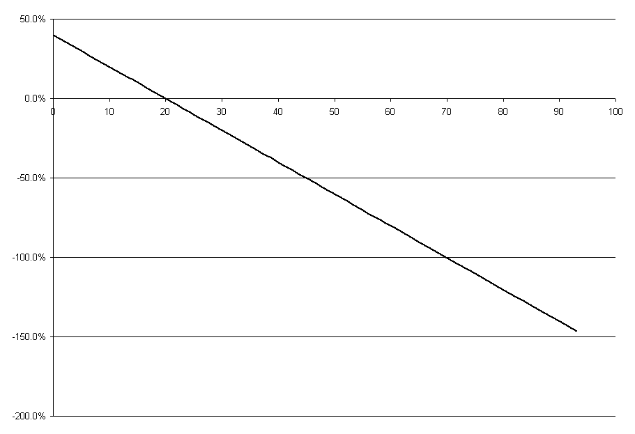
Figure 1. Graph of the function $\beta(S)$

The operator ${\mathcal{V}}_{\mathrm{sv}}(b;b^{\prime}|x,a)$ describes a mean reverting process for stochastic volatility given by volatility regimes. It is allowed to switch between three possible states: low, medium and high. Evidence that the volatility process experiences patters which can be effectively described by means of regimes has been previously discussed by Rebonato and Joshi in [RJ]. The underlying stock price is allowed to transition from one regime to another only between adjacent regimes.

The Markov generator satisfies the following three conditions corresponding to probability positivity and conservation and to arbitrage freedom, respectively:

(3) $${\mathcal{L}}(x,a,b;x^{\prime},a^{\prime},b^{\prime};t)\geq 0\quad\mathrm{if}\quad(x,a,b)\neq(x^{\prime},a^{\prime},b^{\prime})$$

(4) $$\sum_{x^{\prime},a^{\prime},b^{\prime}}{\mathcal{L}}(x,a,b;x^{\prime},a^{\prime},b^{\prime};t)=0$$

(5) $$\sum_{x^{\prime},a^{\prime},b^{\prime}}{\mathcal{L}}(x,a,b;x^{\prime},a^{\prime},b^{\prime};t)(S(x^{\prime})-S(x))=r(t)S(x)$$

The problem of computing the propagator $U(t_{1},t_{2})$ satisfying the backward equation

(6) $$\frac{d}{dt_{1}}U(t_{1},t_{2})+{\mathcal{L}}(t_{1})\,U(t_{1},t_{2})=0$$

with final time condition $U(t_{1},t_{2})=\mathbb{I}$, the identity operator, is solved by exponentiating our generator $\mathcal{L}(t)$

(7) $$U(t_{1},t_{2})=\exp\left(\int_{t_{1}}^{t_{2}}\mathcal{L}(s)ds\right)$$

The matrix exponentiation can be done in a number of ways  [ML]. The method we advocate is the linear fast exponentiation algorithm which we find is fast, stable with respect to floating point errors and can be implemented in single precision on highly efficient GPU platforms.

Fast exponentiation proceeds as follows: Assume that the generators $\mathcal{L}(t)$ are piecewise constant as a function of time. Suppose $\mathcal{L}(t)=\mathcal{L}_{i}$ in the time interval $[t_{i},t_{i}+(\Delta t)_{i}]$. Assume $\delta t$ is chosen to be small enough (but not smaller) that the following two conditions hold:

(8) $$\mathrm{min}_{y\in\Lambda}(1+\delta t\mathcal{L}_{i}(y,y))\geq 1/2$$

(9) $$\log_{2}\frac{(\Delta t)_{i}}{\delta t}=n\in\mathbb{N}$$

This condition leads to intervals $\delta t$ of the order of one hour of calendar time. To compute $e^{(\Delta t)_{i}\mathcal{L}_{i}}(x,y)$, we first define the elementary propagator

(10) $$u_{\delta t}(x,y)=\delta_{xy}+\delta t\mathcal{L}_{i}(y,y)$$

and then evaluate in sequence

(11) $$u_{2\delta t}=u_{\delta t}\cdot u_{\delta t}\,,\,u_{4\delta t}=u_{2\delta t}\cdot u_{2\delta t}\,,\,\dots,u_{2^{n}\delta t}=u_{2^{n-1}\delta t}\cdot u_{2^{n-1}\delta t}$$

The matrix multiplication is accomplished numerically by invoking the level-3 BLAS routine sgemm.

3. The Moment Method

One possible strategy to evaluate moments of path dependent functions is to use Dyson’s formula, see [A]. This formula is sometimes also attributed to Kac  [DK] and provides an expression for moments of integrals of stochastic processes. Moment methods involve reconstructing probability distribution functions for such integrals by extrapolating out of the knowledge of the first few moments. This involves selecting a probability distribution function available in closed form and matching moments.

Consider a time interval $[T,t]$ and a Markov generator $\mathcal{L}(y_{1},y_{2};t)$, and consider the integral $I_{t}$ given by

(12) $$I_{t}=I(y_{t},t)\equiv\int_{T}^{t}\phi(y_{s},s)ds$$

Let’s introduce the following one parameter family of deformed Markov operators parameterized by $\epsilon\in\mathbb{R}$

(13) $$\mathcal{L}_{\epsilon}(y_{1},y_{2};t)=\mathcal{L}(y_{1},y_{2};t)+\epsilon V(y_{1},y_{2};t)$$

where

(14) $$V(y_{1},y_{2};t)=\phi(y_{1};t)\delta_{y_{1},y_{2}}+\mathcal{L}(y_{1},y_{2};t)\chi(y_{1},y_{2};t)(\psi(y_{2};t)-\psi(y_{1};t))$$

The functions $\phi(y;t)$, $\psi(y;t)$ and $\chi(y;t)$ are all continuous functions. We add the $\psi$ and $\chi$ functions here as we can use them to model certain path dependents, however in the applications we describe below we only need the first term $\phi(y;t)$ in order to model the integral in equation (12).

Theorem 1.

For $n=0,1,2,\dots$, we have that

(15) $$\left({d\over d\epsilon}\right)^{n}\bigg{\lvert}_{\epsilon=0}P\exp\bigg{(}\int_{T}^{t}\mathcal{L}_{\epsilon}(s)ds\bigg{)}(y_{1},y_{2})=E_{T}\big{[}I_{t}^{n}\delta(y_{t}-y_{2})\lvert y_{T}=y_{1}\big{]}.$$

Proof.

Consider Neper’s formula for the propagator

(16) $$P\exp\bigg{(}\int_{T}^{t}\mathcal{L}_{\epsilon}(s)ds\bigg{)}=\lim_{N\to\infty}P\prod_{i=1}^{N}\left(1+{t-T\over N}(\mathcal{L}(t_{i})+\epsilon\phi(t_{i}))\right)^{N}$$

where $t_{i}=T+{it\over N}$. By collecting similar powers in $\epsilon$, one finds Dyson’s formula

(17) $$P\exp\bigg{(}\int_{T}^{t}\mathcal{L}_{\epsilon}(s)ds\bigg{)} =\exp((t-T)\mathcal{L}+$$

(18) $$\epsilon\int_{T}^{t}ds_{1}\bigg{(}e^{(s_{1}-T)\mathcal{L}}V(s_{1})e^{(t-s_{1})\mathcal{L}}\bigg{)}+$$

(19) $$\sum_{n=2}^{\infty}\epsilon^{n}\int_{T}^{t}ds_{1}...\int_{s_{n-1}}^{t}ds_{n}\bigg{(}e^{(s_{1}-T)\mathcal{L}}V(s_{1})e^{(s_{2}-s_{1})\mathcal{L}}....V(s_{n})e^{(t-s_{n})\mathcal{L}}\bigg{)}.$$

The time-ordered integrals above are proportional to conditional moments, i.e.

(20) $$P\exp\bigg{(}\int_{T}^{t}\mathcal{L}_{\epsilon}(s)ds\bigg{)}(y_{1},y_{2})=\sum_{n=0}^{\infty}{\epsilon^{n}\over n!}E_{T}\big{[}I_{t}^{n}\delta\big{(}y_{t}-y_{2}\big{)}\lvert y_{T}=y_{1}\big{]}.$$

Here, the factorials originate from the time ordering. ∎

A technique which is numerically stable in many situations of practical relevance is to numerically differentiate with respect to $\epsilon$ the deformed propagators $P\exp\bigg{(}\int_{T}^{t}\mathcal{L}_{\epsilon}(s)ds\bigg{)}(y_{1},y_{2})$ and evaluate at $\epsilon=0$. This technique can be used to obtain the first moments of $I_{t}$ on any given bridge for the underlying Markov process. In most applications, we find that two moments suffice to extrapolate the probability distribution function to sufficient accuracy. To do so, it is convenient to choose from among the probability distribution functions which are analytically tractable. For instance, starting from the first two moments only, one can use either the log-normal or the chi-square distribution. In the above theorem, one only needs to compute the formula for $n$ equal to the number of moments we want to use.

One may notice that Dyson formula in our Finance application is used differently from how it is used in Physics. In Physics one usually has a perturbative method to evaluate moments and the purpose is to reconstruct the kernel. In Finance, fast exponentiation gives a good way to evaluate the kernel and Dyson formula is used to evaluate moments by numerical differentiation.

4. Contracts on Realized Variance

Having introduced a stock price model and a moment formula for path functionals, we next consider volatility derivatives.

A variance swap is a financial contract that upon expiry pays the difference between a capped measure of the historically realized variance of daily stock returns and a fixed swap rate determined at inception. As usual, the swap rate is initially struck at equilibrium so that the variance swap has zero cost to enter [CM].

Variance swaps of maturity $t$ and time of issuance $T$ have a payoff given by

(21) $$\mathrm{min}\left(\frac{1}{t-T}\int_{T}^{t}v(y_{s},s)ds,f\cdot SR^{2}\right)-SR^{2}$$

where $SR$ is the swap rate and $f$ is a factor, a typical value being $f=6.2$. Here, $v(y_{1},t)$ is the instantaneous variance defined as follows:

(22) $$v(y_{1},t)=\sum_{y_{2}}{\mathcal{L}}(y_{1},y_{2};t)\log^{2}\left(\frac{S(y_{2})}{S(y_{1})}\right)$$

The cap is customary on single stocks as, in case of default, realized log-normal variance may actually diverge. Instead, variance swaps on indices are usually uncapped and the equilibrium swap rate is simply given by the first moment

(23) $$\frac{1}{t-T}E_{T}\left[\left.\int_{T}^{t}v(y_{s},s)ds\,\delta\big{(}y_{t}-y_{2}\big{)}\right|y_{T}=y_{1}\right]-SR^{2}.$$

The expectation is given by the first derivative in equation (15) without any need for moment matching. Summing over all final points $y_{2}$ removes the bridge condition on the final points.

The payoff of a volatility swap is

$$\mathrm{min}\left(\sqrt{\frac{1}{t-T}\int_{T}^{t}v(y_{s},s)ds},SR\right)-SR$$

To price these contracts one needs to evaluate the distribution of realized variance on a bridge, i.e. of the functional

(24) $$RV(y_{2})=\delta\left(y_{t}-y_{2}\right)\frac{1}{t-T}\int_{T}^{t}v(y_{s},s)ds$$

In this case, moment matching is required even in case the cap is lifted.

4.1. Matching the moments to a chi-square distribution

Let

$$m_{1}=E_{T}\big{[}I_{t}\left.\delta\big{(}y_{t}-y_{2}\big{)}\right|y_{T}=y_{1}\big{]}\quad\quad\mathrm{and}\quad\quad m_{2}=E_{T}\big{[}I_{t}^{2}\left.\delta\big{(}y_{t}-y_{2}\big{)}\right|y_{T}=y_{1}\big{]}$$

be our first and second pre-assigned moments. The standard chi-square distribution is given by

$$f(x)=\frac{1}{2\Gamma\left(\frac{a}{2}\right)}\left(\frac{x}{2}\right)^{a/2-1}e^{-x/2}$$

where $a$ is the number of degrees of freedom. The first and second moments of this distribution are

$$E[x]=a\,,\,\,\,\,\,\,\,\,\,\,\,\,\,E[x^{2}]=a(a+2)$$

To match two pre-assigned moments $m_{1}$, $m_{2}$, one can pass to the new variable

$$\xi=\frac{m_{1}}{a}x$$

and chose

$$a=\frac{2m_{1}^{2}}{m_{2}-m_{1}^{2}}$$

The cumulative distribution function is

$$F(x;a)=\frac{\gamma\left(\frac{a}{2},\frac{x}{2}\right)}{\Gamma\left(\frac{a}{2}\right)},$$

where $\Gamma(z)$ and $\gamma(z,a)$ are the gamma and incomplete gamma functions respectively, i.e:

$$\Gamma(z)=\int_{0}^{\infty}s^{z-1}e^{-s}ds\,,\,\,\,\,\,\gamma(z,a)=\int_{0}^{a}s^{z-1}e^{-s}ds.$$

We find that

$$E_{T}\left[\mathrm{min}(RV,RV_{\mathrm{max}})\,\delta(y_{t}-y_{2})\right]=\frac{m_{1}}{a}\left[K(1-F(K;a))+aF(K;a+2)\right]$$

and

$$E_{T}\left[\mathrm{min}(\sqrt{RV},\sqrt{RV_{\mathrm{max}}})\,\delta(y_{t}-y_{2})\right]=\sqrt{\frac{m_{1}}{a}}\left[\sqrt{K}(1-F(K;a))+\frac{\sqrt{2}\gamma\left(\frac{a+1}{2},\frac{K}{2}\right)}{\Gamma\left(\frac{a}{2}\right)}\right]$$

where

$$a=a(y_{1},y_{2})=\frac{2m_{1}(y_{1},y_{2})^{2}}{m_{2}(y_{1},y_{2})-m_{1}(y_{1},y_{2})^{2}}\,,\,\,\,\,K=K(y_{1},y_{2})=\frac{a(y_{1},y_{2})}{m_{1}(y_{1},y_{2})}RV_{\mathrm{max}}$$

These formulas allow one to price both variance swaps and volatility swaps. Since the dependency on the swap rate in both cases is non-linear, an exact calculation requires using a root finder. This may be avoided as an excellent approximation is often obtained by estimating the variance swap rate as follows:

(25) $$VARSR_{T}=\sqrt{\sum_{y_{2}}E_{T}[\mathrm{min}(RV,RV_{\mathrm{max}})\,\delta(y_{t}-y_{2})]}$$

and the volatility swap rate as follows:

(26) $$VOLSR_{T}=\sum_{y_{2}}E_{T}\left[\mathrm{min}(\sqrt{RV},\sqrt{RV_{\mathrm{max}}})\,\delta(y_{t}-y_{2})\right]$$

where

(27) $$RV_{\mathrm{max}}=f\sum_{y_{3}}U(y_{T},T;y_{3},t)m_{2}(y_{T},y_{3})$$

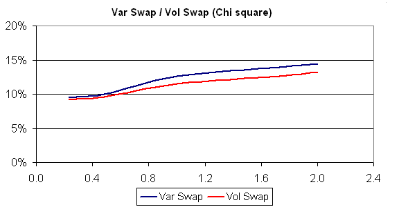
Figure 2. Volatility and variance swaps (Chi-square)

4.2. Matching the moments to a log-normal distribution

Let $x$ be log-normally distributed with probability distribution function

$$f(x;\mu,\sigma)=\frac{1}{x\sigma\sqrt{2\pi}}e^{-(\ln x-\mu)^{2}/2\sigma^{2}}$$

then the first two moments are given by

$$E[x]=e^{\mu+\sigma^{2}/2}\,\,\,\,\,\,\,\,\,\,\,\textrm{and}\,\,\,\,\,\,\,\,\,\,\,E[x^{2}]=e^{2\mu+2\sigma^{2}}.$$

Given these expected values, we can obtain relationships for $\mu$ and $\sigma$ as

(28) $$\mu=\log\left(\frac{E[x]^{2}}{\sqrt{E[x^{2}]}}\right)\,\,\,\,\,\,\,\,\,\,\textrm{and}\,\,\,\,\,\,\,\,\,\,\,\sigma^{2}=\log\left(\frac{E[x^{2}]}{E[x]^{2}}\right)$$

and take the pre-assigned moments to be equal to these expected values $E[x]=m_{1}$ and $E[x^{2}]=m_{2}$. We obtain

$$E_{T}[\mathrm{min}(RV,RV_{\mathrm{max}})\,\delta(y_{t}-y_{2})]$$

expressed in terms of the well known standard normal cumulative distribution function as

(29) $$e^{\mu+\sigma^{2}/2}{\mathcal{N}}\left(\frac{\log(RV_{\mathrm{max}})-\mu-\sigma^{2}/2}{\sigma}\right)+RV_{\mathrm{max}}\,{\mathcal{N}}\left(\frac{\log(RV_{\mathrm{max}})-\mu}{\sigma}\right)$$

and the second expectation is

$$E_{T}\left[\mathrm{min}(\sqrt{RV},\sqrt{RV_{\mathrm{max}}})\,\delta(y_{t}-y_{2})\right]=$$

(30) $$e^{\frac{1}{8}(4\mu+\sigma^{2})}{\mathcal{N}}\left(\frac{\log(RV_{\mathrm{max}})-\mu-\sigma^{2}/2}{\sigma}\right)+\sqrt{RV_{\mathrm{max}}}\,{\mathcal{N}}\left(\frac{\log(RV_{\mathrm{max}})-\mu}{\sigma}\right)$$

where $\mu$ and $\sigma$ are specified above in terms of $m_{1}$ and $m_{2}$.

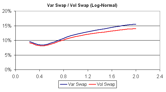
Figure 3. Volatility and variance swaps (log-normal)

4.3. Matching higher moments with the Pearson distributions

The log-normal and the chi-square distributions allow us to match the first two moments, here we look at three. Consider the Pearson Type III distribution which has probability distribution function

$$f(x)=\frac{1}{b\Gamma(p)}\left(\frac{x-a}{b}\right)^{p-1}e^{-(x-a)/b}$$

defined on $[a,+\infty)$. The special case of this, when $a=0$, $b=2$ and $p$ is half of an integer, gives the Chi-Squared distribution. In general, the moments are given by

(31) $$E[x]=a+bp$$

$$E[x^{2}]=(a+bp)^{2}+b^{2}p$$

$$E[x^{3}]=(a+bp)^{3}+3b^{2}p(a+bp)+2b^{3}p$$

and matching these with our pre-assigned moments $m_{1},m_{2}$ and $m_{3}$ and computing the values of $a,b$ and $p$ in terms of these moments we find

(32) $$a=m_{1}-\frac{2(m_{2}-m_{1}^{2})^{2}}{m_{3}+2m_{1}^{3}-3m_{1}m_{2}}$$

$$b=\frac{m_{3}+2m_{1}^{3}-3m_{1}m_{2}}{2(m_{2}-m_{1}^{2})}$$

$$p=\frac{4(m_{2}-m_{1}^{2})^{3}}{(m_{3}+2m_{1}^{3}-3m_{1}m_{2})^{2}}$$

Then the expectation in concern, expressed in terms of the chi-squared cumulative distribution function $F(x;a)$ (section  4.1) is

$$E_{T}\left[\mathrm{min}(RV,RV_{\mathrm{max}})\,\delta(y_{t}-y_{2})\right]=(a+bp-RV_{\mathrm{max}})F_{\mathrm{Chi}}\left(2p,2\frac{RV_{\mathrm{max}}-a}{b}\right)$$

(33) $$-b\left(\frac{RV_{\mathrm{max}}-a}{b}\right)^{p}\frac{e^{-\frac{RV_{\mathrm{max}}-a}{b}}}{\Gamma(p)}+(2RV_{\mathrm{max}}-a-bp)$$

5. Corridor Variance Swaps

Corridor variance swaps differ from standard variance swaps in that the underlying s price must be inside a specified corridor in order for its squared return to be included in the floating part of the variance swap payout [CL].

Corridor variance swap are sometimes engineered so that they afford full protection against situations where the variance spikes accompanied by a decline in stock value, but offer only limited protection in case the volatility surge is associated to a stock price rally. Following [CL], one could achieve a robust static replication by means of a strip of options as in the case of the variance swap, only that here the hedge is limited to the pre-specified corridor.
The payoff of corridor variance swaps are given by

(34) $$\frac{1}{t-T}\int_{T}^{t}v(y_{s},s)\,\mathbf{1}(L<S(y_{s})<H)ds-SR^{2}$$

so we are interested in the integral

$$I_{t}=\frac{1}{t-T}\int_{T}^{t}\phi(y_{s},s)ds$$

where

(35) $$\phi(y_{1},t)=\sum_{y_{2}}{\mathcal{L}}(y_{1},y_{2};t)\log^{2}\left(\frac{S(y_{2})}{S(y_{1})}\right)\mathbf{1}(L<S(y_{2})<H)$$

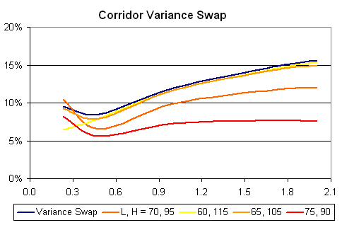
Figure 4. Corridor Variance Swaps

is the ”instantaneous corridor variance”, and solve the problem of computing its moments by specifying in this case the operator

$${\mathcal{L}}_{\epsilon}(y_{1},y_{2};t)={\mathcal{L}}(y_{1},y_{2};t)+\epsilon\phi(y_{1},t)\delta_{y_{1}y_{2}}.$$

From here the methodology used in the case of ordinary variance swaps carries through and one is reduced to computing and matching moments.

6. Conditional Variance Swaps

Conditional corridor variance swaps are an interesting variant as they can more easily be interpreted in intuitive terms. In this case, the payoff is given by the accrued variance divided by the time elapsed in the range, not the total number of days  [JP]. Namely, the payoff is given by

(36) $$\frac{\int_{T}^{t}v(y_{s},s)\,\mathbf{1}(L<S(y_{s})<H)ds}{\int_{T}^{t}\mathbf{1}(L<S(y_{s})<H)ds}-SR^{2}$$

The principal use of conditional derivatives is when an investor expects a particular asset (e.g. market level, volatility) to outperform contingent on a level of another asset being breached. In the case of a conditional variance swap, the investor may be anticipating that volatility will increase/decrease if the market were to rally/sell-off or stay within a range [JP]. While an investor can select the corridor freely, two examples are the conditional up-variance and down-variance swaps. Up-variance accrues realised variance only when the underlying is above a pre-specified level (i.e. no upper barrier), while down-variance is accrued only when the underlying is below the specified barrier (i.e. no lower barrier).

To apply the moment method to this case, the first thing to note is that essentially we are modelling the two integrals appearing in the payoff at the same time. We are going to need a bi-variate distribution to do this. Let’s write:

$$I_{t}^{(1)}=\int_{T}^{t}v(y_{s},s)\,\mathbf{1}(L<S(y_{s})<H)ds$$

$$I_{t}^{(2)}=\int_{T}^{t}\mathbf{1}(L<S(y_{s})<H)ds$$

and in order to compute the expectation

(37) $$E\left[\frac{I_{t}^{(1)}}{I_{t}^{(2)}}\right]$$

we’ll need the following expectations:

$$E\left[I_{t}^{(1)}\right]\,,\,\,\,\,E\left[I_{t}^{(2)}\right]\,,\,\,\,\,E\left[\left(I_{t}^{(1)}\right)^{2}\right]\,,\,\,\,\,E\left[\left(I_{t}^{(2)}\right)^{2}\right]\,,\,\,\,\,\mathrm{and}\,\,\,\,\,\,E\left[I_{t}^{(1)}I_{t}^{(2)}\right]$$

To tackle this problem consider the operator

(38) $${\mathcal{L}}_{\epsilon_{1},\epsilon_{2}}(y_{1},y_{2})={\mathcal{L}}(y_{1},y_{2})+\epsilon_{1}\phi(y_{1})\delta_{y_{1}y_{2}}+\epsilon_{2}\,\psi(y_{1})\delta_{y_{1}y_{2}}$$

where

(39) $$\phi(y_{1},t)=\sum_{y_{2}}{\mathcal{L}}(y_{1},y_{2};t)\log^{2}\left(\frac{S(y_{2})}{S(y_{1})}\right)\mathbf{1}(L<S(y_{1})<H)$$

and

(40) $$\psi(y_{1})=\mathbf{1}(L<S(y_{1})<H)$$

then the problem of computing these moments is solved using the above procedure. In particular, we have

$$\left.\frac{\partial}{\partial\epsilon_{1}}\right|_{\epsilon_{1}=0}e^{((t-T){\mathcal{L}}_{\epsilon_{1},\epsilon_{2}})}(y_{1},y_{2})=E\left[\left.I_{t}^{(1)}\right|y_{T}=y_{1},y_{t}=y_{2}\right]$$

and

$$\left.\frac{\partial^{2}}{\partial\epsilon_{1}^{2}}\right|_{\epsilon_{1}=0}e^{((t-T){\mathcal{L}}_{\epsilon_{1},\epsilon_{2}})}(y_{1},y_{2})=E\left[\left.\left(I_{t}^{(1)}\right)^{2}\right|y_{T}=y_{1},y_{t}=y_{2}\right]$$

similarly (but with respect to $\epsilon_{2}$) for

$$E\left[\left.I_{t}^{(2)}\right|y_{T}=y_{1},y_{t}=y_{2}\right]\,\,\,\,\,\,\,\mathrm{and}\,\,\,\,\,\,\,E\left[\left.\left(I_{t}^{(2)}\right)^{2}\right|y_{T}=y_{1},y_{t}=y_{2}\right]$$

The joint expectation will involve the mixed derivative:

(41) $$E\left[I_{t}^{(1)}I_{t}^{(2)}\right]=\left.\frac{\partial^{2}}{\partial\epsilon_{1}\partial\epsilon_{2}}\right|_{\epsilon_{1},\epsilon_{2}=0}e^{((t-T){\mathcal{L}}_{\epsilon_{1},\epsilon_{2}})}(y_{1},y_{2})$$

and once computed, we make use of these expectations to match a bivariate distribution. For simplicity of notation we leave out the conditional part of these expectations, noting that all the moments we obtain are conditional to the initial and final points.

6.1. Bi-Variate log-normal distribution:

Let

$$\left(\begin{array}[]{c}Y_{1}\\ Y_{2}\\ \end{array}\right)=\left(\begin{array}[]{c}\log(X_{1})\\ \log(X_{2})\\ \end{array}\right)\sim N\left(\left(\begin{array}[]{c}\mu_{1}\\ \mu_{2}\\ \end{array}\right),\left(\begin{array}[]{c}\sigma_{1}\\ \sigma_{2}\\ \end{array}\right)\right)$$

then $X_{1}$ and $X_{2}$ have joint probability distribution function  [JK]:

(42) $$f(x_{1},x_{2})=\frac{1}{2\pi\sigma_{1}\sigma_{2}\sqrt{1-\rho^{2}}x_{1}x_{2}}\cdot$$

$$\exp\left\{-\frac{1}{2(1-\rho^{2})}\left[\left(\frac{\log x_{1}-\mu_{1}}{\sigma_{1}}\right)^{2}-2\rho\frac{(\log x_{1}-\mu_{1})(\log x_{2}-\mu_{2})}{\sigma_{1}\sigma_{2}}+\left(\frac{\log x_{2}-\mu_{2}}{\sigma_{2}}\right)^{2}\right]\right\}$$

the bivariate log-normal distribution, where $\rho$ is the correlation between $X_{1}$ and $X_{2}$. Both $X_{1}$ and $X_{2}$ are log-normally distributed with

$$E[X_{i}]=e^{\mu_{i}+\sigma_{i}^{2}/2}\,,\,\,\,\,\,\,\,\mathrm{and}\,\,\,\,\,\,E[X_{i}^{2}]=e^{2\mu_{i}+2\sigma_{i}^{2}}\,,\,\,\,\,i=1,2.$$

Matching these with the pre-assigned moments, and solving for $\mu_{i}$ and $\sigma_{i}$ we find (similarly to section 4.2)

$$\mu_{i}=\log\left(E\left[I_{t}^{(i)}\right]^{2}\Big{/}\,\sqrt{E\left[\left(I_{t}^{(i)}\right)^{2}\right]}\right)\,\,\,\,\,\,\,\textrm{and}\,\,\,\,\,\,\,\,\,\sigma_{i}^{2}=\log\left(E\left[\left(I_{t}^{(i)}\right)^{2}\right]\Big{/}\,E\left[\left(I_{t}^{(i)}\right)\right]^{2}\right)$$

Moreover, the mixed term is

$$E\left[X_{1}X_{2}\right]=E\left[e^{Y_{1}+Y_{2}}\right]=e^{\mu_{1}+\mu_{2}+\frac{1}{2}(\sigma_{1}^{2}+\sigma_{2}^{2}+2\rho\sigma_{1}\sigma_{2})}=E[X_{1}]E[X_{2}]\,e^{\rho\sigma_{1}\sigma_{2}}$$

which gives $\rho$ (in terms of the pre-assigned moments):

(43) $$\rho=\frac{1}{\sigma_{1}\sigma_{2}}\log\frac{E\left[I_{t}^{(1)}I_{t}^{(2)}\right]}{E\left[I_{t}^{(1)}\right]E\left[I_{t}^{(2)}\right]}$$

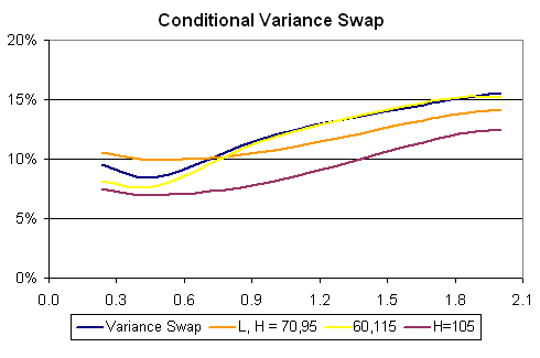
Figure 5. Conditional Variance Swaps: A standard variance swap, two conditional variance swaps of different corridors, and a 105% (of spot) conditional up-variance swap.

Now we are in a position to compute the expectation $E\left[I_{t}^{(1)}\Big{/}\,I_{t}^{(2)}\right]$. Given the bivariate log-normal distribution, we have

$$E\left[\frac{X_{1}}{X_{2}}\right]=E\left[e^{Y_{1}-Y_{2}}\right]=E\left[e^{Y_{1}+Y^{{}^{\prime}}_{2}}\right]$$

where $Y^{{}^{\prime}}_{2}=-Y_{2}$ will also be normally distributed $\sim N(-\mu_{2},\sigma_{2}^{2})$, so

$$E\left[\frac{X_{1}}{X_{2}}\right]=e^{\mu_{1}+\frac{1}{2}\sigma_{1}^{2}}\,e^{-\mu_{2}+\frac{1}{2}\sigma_{2}^{2}}\,e^{-\rho\sigma_{1}\sigma_{2}}$$

and the expectation (37) is given by

(44) $$E\left[\frac{I_{t}^{(1)}}{I_{t}^{(2)}}\right]=E\left[I_{t}^{(1)}\right]\cdot\frac{E\left[\left(I_{t}^{(2)}\right)^{2}\right]}{E\left[I_{t}^{(2)}\right]^{3}}\cdot\frac{E\left[I_{t}^{(1)}\right]E\left[I_{t}^{(2)}\right]}{E\left[I_{t}^{(1)}I_{t}^{(2)}\right]}=\frac{E\left[I_{t}^{(1)}\right]^{2}E\left[\left(I_{t}^{(2)}\right)^{2}\right]}{E\left[I_{t}^{(2)}\right]^{2}E\left[I_{t}^{(1)}I_{t}^{(2)}\right]}$$

Plugging this in the payoff of the conditional variance swap (36) gives us the value of the conditional variance swap.

We could go a step further and compute the analogy of the capped variance swap in equation (21) where we are now interested in the payoff $E\left[\mathrm{min}\left(\frac{X_{1}}{X_{2}},CV_{\mathrm{Max}}\right)\right]$. Writing this expectation as a double integral over the bi-variate probability distribution function (42) we find

(45) $$E\left[\mathrm{min}\left(\frac{X_{1}}{X_{2}},CV_{\mathrm{Max}}\right)\right]=\int_{0}^{\infty}\int_{0}^{X_{2}CV_{\mathrm{Max}}}\left(\frac{X_{1}}{X_{2}}-CV_{\mathrm{Max}}\right)f(X_{1},X_{2})dX_{1}dX_{2}+CV_{\mathrm{Max}}$$

This double integral will need to be evaluated numerically; one could apply a Gaussian quadrature.

7. Gamma Swaps and Variance Knockouts

In this section, we apply the moment method to other volatility contracts, namely options on realized variance, variance knock-out options and gamma swaps.

7.1. Options on Realized Variance

Let’s consider the example of a call option on realized variance, we are interested in the payout $E\left[(RV-K)^{+}\right]$. Computing the conditional moments for the realized variance as described above, we can sum over all final points $y_{2}$ to obtain the unconditional moments. Matching these with a distribution we know, as done above, we can look at the payoff

(46) $$E_{T}\left[(RV-K)^{+}\right]$$

which under the log-normal case is given by the Black-Scholes formula, with the correct inputs from equation (28).

7.2. Variance Knock-out Options

The payoff of a variance knockout call-option with volatility barrier at $H$ is

(47) $$(D(T)S_{T}-K)_{+}\mathbf{1}\left(\frac{1}{t-T}\int_{T}^{t}v(y_{s},s)ds<H^{2}\right)$$

Variance conditional knock-out options are priced as follows:

(48) $$VKO_{T}=\sum_{y_{2}}U(y_{T},T;y_{2},t)\,\mathbf{Pr}\left(RV(y_{2})<H^{2}\right)\left(D(T^{\prime})S(y_{2},t)-K\right)_{+}$$

where $\mathbf{Pr}\left(RV(y_{2})<H^{2}\right)$, the probability that $RV(y_{2})<H^{2}$ is obviously the cumulative distribution function (for the distribution which we chose to model $RV$ with).

7.3. Gamma swaps

The gamma swap (also known as weighted variance swap) is similar to the variance swap only we have an additional spot factor. They reduce the weighting of the downside scenarios but introduce a market level exposure. The gamma variance swap pays at maturity the realized weighted variance of an asset

$$\frac{252}{m}\sum_{i}^{n}\log\left(\frac{S_{i}}{S_{i-1}}\right)^{2}\frac{S_{i}}{S_{0}}$$

We note the following features of the Gamma swap
(i) As the spot approaches zero, we do not have a blow up as in the case of the variance swap: $\lim_{x\to 0}x\log(x)=0$,
(ii) Similar to the variance swap case, one can split the gamma swap payoff into a European payoff and a daily hedging strategy. However in the case of the Gamma swap, the weights in the replicating portfolio are of order $1/K$ compared to those in the variance swap of order $1/K^{2}$.

To price the gamma swap within our framework, we look at the instantaneous level: we no longer have the instantaneous variance, but the ”instantaneous gamma” given by

$$g(y_{1},t)=\sum_{y_{2}}{\mathcal{L}}(y_{1},y_{2};t)\log^{2}\left(\frac{S(y_{2})}{S(y_{1})}\right)\frac{S(y_{2})}{S(y_{1})}$$

Gamma swaps of maturity $t$ and time of issuance $T$ have a payoff given by

(49) $$\frac{1}{t-T}\int_{T}^{t}g(y_{s},s)ds-SR^{2}$$

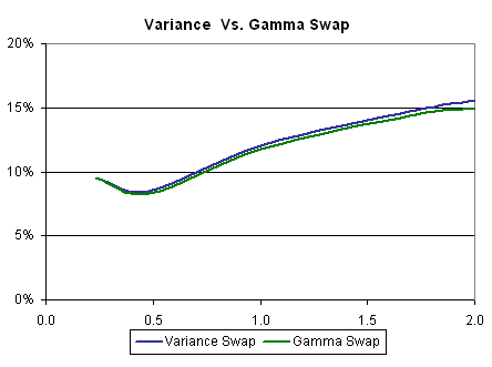
Figure 6. Gamma swap

8. Summary and extensions

Using operator theory we presented a 3-factor equity model which is semi-parametric or even non-parametric and allows for a time-homogeneous calibration. A moment method based on Dyson’s formula is then given and used to compute the moments of integrals of the underlying Markov process. We then apply this method to a various volatility derivatives which we find to be well suited to moment methods. We consider a number of exotics such as variance knockouts, conditional corridor variance swaps, variance swaptions and gamma swaps. Straightforward extensions would include for instance conditional corridor variance knockout options, forward starting variance swaptions, etc..

References

- [1] \harvarditem[Albanese]Albanese2006A Albanese, C. (2006). Operator Methods, Abelian Processes and Dynamic Conditioning. preprint, available at www.level3finance.com.
- [2] \harvarditem[Carr and Madan]Carr and Madan1998CM Carr, P. and D. Madan (1998). Towards a theory of volatility trading. Volatility, Risk Publications, ed. Jarrow, R.
- [3] \harvarditem[Carr and Lewis]Carr and Lewis2004CL Carr, P. and K. Lewis (2004). Corridor variance swaps. Risk February, 67–72.
- [4] \harvarditem[Carr and Lee]Carr and Lee2007CLee Carr, P. and R. Lee (2007). Realized Volatility and Variance: Options via Swaps. Risk.
- [5] \harvarditem[Darling and Kac]Darling and KacMar., 1957DK Darling, D. A. and M. Kac (Mar., 1957). On occupation times for markoff processes. Transactions of the American Mathematical Society 84, 444–458.
- [6] \harvarditem[Derman et al.]Derman et al.1999DDKZ Derman, E., K. Demeterfi, M. Kamal and J. Zou (1999). More Than You Ever Wanted to Know about Volatility Swaps. Journal of Derivatives.
- [7] \harvarditem[Dupire]Dupire1992D1992 Dupire, B. (1992). Arbitrage Pricing with Stochastic Volatility. preprint, Soci t G n rale.
- [8] \harvarditem[Johnson and Kotz]Johnson and Kotz1942JK Johnson, N.L. and S. Kotz (1942). Continuous multivariate distributions. John Wiley and Sons.
- [9] \harvarditem[J.P. Morgan Securities]J.P. Morgan Securities2006JP J.P. Morgan Securities (2006). Conditional variance swaps, product note. Technical report.
- [10] \harvarditem[Moler and Loan]Moler and Loan2003ML Moler, C. and C.V. Loan (2003). Nineteen dubious ways to compute the exponential of a matrix, twenty-five years later. SIAM Review pp. 3–30.
- [11] \harvarditem[Rebonato and Joshi]Rebonato and Joshi2001RJ Rebonato, R. and M. Joshi (2001). A joint empirical and theoretical investigation of the modes of deformation of swaption matrices: implications for model choice. QUARC Working paper.
- [12]