First quenched results for the matrix elements of the $B_{B_{s}}$ mixing parameter in the static limit from tmQCD

Abstract:

We report on a non-perturbative study of the scale-dependent renormalization factors of a multiplicatively renormalizable basis of $\Delta B=2$ parity-odd four-fermion operators in quenched lattice QCD. We also present some preliminary results of the matrix elements related to the mixing parameter of the $B_{s}$-meson. In our lattice formulation, the heavy quark is treated in the static approximation, while the strange one belongs to a doublet of twisted mass fermions at full twist, i.e. with twist angle $\alpha=\pi/2$. In this framework, the parity-even $\Delta B=2$ four-fermion operators responsible for the mixing are rotated onto a linear combination of parity-odd operators in the above-mentioned basis. Their physical matrix elements between static $B_{s}$-mesons are extracted from lattice correlators with Schrödinger functional boundary conditions. We observe a suppression of excited state contributions to the $B_{B_{s}}$ mixing parameter and speculate about possible explanations.

1 Introduction

Currently, theoretical determinations of the mixing parameters $B_{B_{q}}$ ($q=d,s$) are becoming more and more urgent in relation to the Unitarity Triangle analysis. The $B$-parameters are defined as the relative deviations from the Vacuum Saturation Approximation (VSA) of the matrix elements of $\Delta B=2$ four-fermion operators between $B$-meson states, i.e.

$$B_{B_{q}}=\frac{\langle\bar{B}^{0}_{q}|{\cal O}^{\scriptscriptstyle\Delta B=2}_{\rm\scriptscriptstyle LL}|B^{0}_{q}\rangle}{\frac{8}{3}f_{B_{q}}^{2}m_{B_{q}}^{2}}\ ,\qquad{\cal O}^{\scriptscriptstyle\Delta B=2}_{\rm\scriptscriptstyle LL}=\left[\bar{\psi}_{b}\gamma_{\mu}(1-\gamma_{5})\psi_{q}\right]\left[\bar{\psi}_{b}\gamma_{\mu}(1-\gamma_{5})\psi_{q}\right]\ .$$ (1)

They encode the low-energy information related to particle-antiparticle oscillations and are formally accessible to lattice QCD simulations. Nevertheless, a direct computation of $B_{B_{q}}$ is hampered by the presence of the large value of the $b$-quark mass, which imposes the adoption of tiny lattice spacings $\left(a\ll 1/(5{\rm GeV})\right)$ in order to avoid large lattice artefacts. A possible way out is to expand the $B$-parameters in Heavy Quark Effective Theory (HQET), i.e. in inverse powers of the $b$-quark mass. The leading contribution, also known as the static approximation, is expected not to be far from the relativistic value, as previous lattice results have shown. Even so, the naïve lattice discretization of the effective four-fermion operators of the static theory, based on Wilson-type light fermions, is affected by a non-trivial renormalization mixing, due to the explicit breaking of chiral symmetry, which pushes the numerics up to the edge of our current technology. Although Ginsparg-Wilson fermions appear as the natural discretization to study left-left four-quark operators, we follow a computationally cheaper approach, based on twisted mass QCD (tmQCD) [1], which allows for purely multiplicative renormalization at the same computational cost as with Wilson quarks.

2 Computational strategy

Our starting point is the equation relating the left-left operator of the fully relativistic theory to the four-fermion operators of HQET,

$$\hskip-22.76228pt{\cal O}^{\scriptscriptstyle\Delta B=2}_{\rm\scriptscriptstyle LL}(m_{b})=\ \ C_{1}(m_{b},\mu)Q_{1}(\mu)+C_{2}(m_{b},\mu)Q_{2}(\mu)+O\left(\frac{1}{m_{b}}\right)\ ,\\$$ (2)

$$\hskip 74.54607ptQ_{1} \ =\ {\cal O}^{\rm stat}_{\rm\scriptscriptstyle VV+AA} \ =\ \left(\bar{\psi}_{h}\gamma_{\mu}\psi_{q}\right)\left(\bar{\psi}_{\bar{h}}\gamma_{\mu}\psi_{q}\right)+\left(\bar{\psi}_{h}\gamma_{\mu}\gamma_{5}\psi_{q}\right)\left(\bar{\psi}_{\bar{h}}\gamma_{\mu}\gamma_{5}\psi_{q}\right)\ ,$$ (3)

$$Q_{2} \ =\ {\cal O}^{\rm stat}_{\rm\scriptscriptstyle SS+PP} \ =\ \left(\bar{\psi}_{h}\psi_{q}\right)\left(\bar{\psi}_{\bar{h}}\psi_{q}\right)+\left(\bar{\psi}_{h}\gamma_{5}\psi_{q}\right)\left(\bar{\psi}_{\bar{h}}\gamma_{5}\psi_{q}\right)\ .$$ (4)

Eq. (2) has to be understood as a scheme dependent perturbative matching between two renormalizable field theories. The coefficients $C_{i}$, known at NLO in the ${\overline{\rm MS}}$/NDR scheme [2], provide the RG evolution from the defining scale $m_{b}$ of the effective theory down to a scale $\mu\approx 1\ {\rm GeV}$. Although a natural hierarchy $\mu<m_{b}$ has to be assumed in the matching equation, it should be observed that, due to the renormalizability of the static theory, the four-fermion operators $Q_{1,2}$ are perfectly defined at any scale. In particular, they can be perturbatively evolved up to the RGI point through the appropriate $2\times 2$ static anomalous dimension matrix, i.e.

$$\left[\begin{array}[]{c}Q_{1}^{\rm\scriptscriptstyle RGI}\\ Q_{2}^{\rm\scriptscriptstyle RGI}\end{array}\right]={\hat{c}}(\mu)\left[\begin{array}[]{c}Q_{1}(\mu)\\ Q_{2}(\mu)\end{array}\right]\ ,$$ (5)

where ${\hat{c}}(\mu)$ will be defined later.

The advantage of introducing RGI operators is twofold. On the one hand, they are truly non-perturbative quantities, free of systematic uncertainties related to perturbative truncations. On the other, they are regularization independent. As such they can be linked to any specific lattice regularization, to be chosen on the basis of computational convenience. A simplification of the renormalization pattern is achieved if we perform a change of basis, i.e. we introduce the primed operators

$$\left[\begin{array}[]{c}Q_{1}^{\prime\rm\scriptscriptstyle RGI}\\ Q_{2}^{\prime\rm\scriptscriptstyle RGI}\end{array}\right]=\left[\begin{array}[]{c}Q_{1}^{\rm\scriptscriptstyle RGI}\\ Q_{1}^{\rm\scriptscriptstyle RGI}+4Q_{2}^{\rm\scriptscriptstyle RGI}\end{array}\right]=\left[\begin{array}[]{cc}1&0\\ 1&4\end{array}\right]\left[\begin{array}[]{c}Q_{1}^{\rm\scriptscriptstyle RGI}\\ Q_{2}^{\rm\scriptscriptstyle RGI}\end{array}\right]={\cal R}\left[\begin{array}[]{c}Q_{1}^{\rm\scriptscriptstyle RGI}\\ Q_{2}^{\rm\scriptscriptstyle RGI}\end{array}\right]\ .$$ (6)

This redefinition becomes particularly advantageous on the lattice if the relativistic degrees of freedom are discretized according to tmQCD at full twist, i.e. with twist angle $\alpha=\pi/2$ [1]. In particular, from now on we consider the specific case of the $B_{s}$-meson, for which we assume a fermion content made of a static quark plus a twisted strange quark belonging to a fully twisted $(c,s)$-doublet. Lighter degrees of freedom, i.e. the up and down quarks, do not need to be further specified, since they do not enter the valence sector. In tmQCD the operators $Q_{1,2}^{\prime}$ are mapped onto their odd parity counterparts ${\cal Q}_{1,2}^{\prime}$, which renormalize purely multiplicatively, as proved in [3]. In other words, with some abuse of notation

$$\langle Q_{1}^{\prime\rm RGI}\rangle =\lim_{a\to 0}{\hat{Z}}^{\prime}_{1,\rm RGI}\left(g_{0}(a)\right)\langle{\cal Q}_{1}^{\prime}(a)\rangle_{\rm tmQCD}^{\alpha=\pi/2}\ ,$$

$$\langle Q_{2}^{\prime\rm RGI}\rangle =\lim_{a\to 0}{\hat{Z}}^{\prime}_{2,\rm RGI}\left(g_{0}(a)\right)\langle{\cal Q}_{2}^{\prime}(a)\rangle_{\rm tmQCD}^{\alpha=\pi/2}\ ,$$ (7)

where

$$\hskip-113.81102pt{\cal Q}^{\prime}_{1} \ =\ {\cal O}_{\rm\scriptscriptstyle VA+AV} \ =\ \left(\bar{\psi}_{h}\gamma_{\mu}\psi_{q}\right)\left(\bar{\psi}_{\bar{h}}\gamma_{\mu}\gamma_{5}\psi_{q}\right)+\left(\bar{\psi}_{h}\gamma_{\mu}\gamma_{5}\psi_{q}\right)\left(\bar{\psi}_{\bar{h}}\gamma_{\mu}\psi_{q}\right)\ ,$$ (8)

$${\cal Q}^{\prime}_{2} \ =\ {\cal O}_{\rm\scriptscriptstyle VA+AV}+4{\cal O}_{\rm\scriptscriptstyle PS+SP} \ =\ \left(\bar{\psi}_{h}\gamma_{\mu}\psi_{q}\right)\left(\bar{\psi}_{\bar{h}}\gamma_{\mu}\gamma_{5}\psi_{q}\right)+\left(\bar{\psi}_{h}\gamma_{\mu}\gamma_{5}\psi_{q}\right)\left(\bar{\psi}_{\bar{h}}\gamma_{\mu}\psi_{q}\right)+$$

$$4\left[\left(\bar{\psi}_{h}\gamma_{5}\psi_{q}\right)\left(\bar{\psi}_{\bar{h}}\psi_{q}\right)+\left(\bar{\psi}_{h}\psi_{q}\right)\left(\bar{\psi}_{\bar{h}}\gamma_{5}\psi_{q}\right)\right]\ .$$ (9)

The RGI renormalization constants ${\hat{Z}}^{\prime}_{k,\rm RGI}$ $(k=1,2)$ have been recently obtained in the quenched approximation [4] through finite size techniques based on the Schrödinger functional [5]. Since the latter allows for the adoption of mass independent schemes, the computation of ${\hat{Z}}^{\prime}_{k,\rm RGI}$ has been performed with standard (untwisted) Wilson fermions. A preliminary study of the non-perturbative renormalization for $N_{\rm f}=2$ has been also presented at this conference [6].

3 Non-perturbative renormalization in the Schrödinger functional

In order to study the renormalization of the four-quark operators, we consider a theory with a light quark sector consisting of two massless ${\rm O}(a)$ improved Wilson-type quarks $(\psi_{1},\psi_{2})$ entering the four-quark operators, plus a third light spectator quark $\psi_{3}$, regularized in the same way, whose rôle will be clarified in a moment. Suitable renormalization conditions can be specified in terms of SF correlators made of bilinear boundary source operators $\Sigma_{s_{1}s_{2}}$, $\Sigma^{\prime}_{s_{1}s_{2}}$ (lying resp. on the two time boundaries $x_{0}=0$ and $x_{0}=T$)

$$\Sigma_{s_{1}s_{2}}[\Gamma]=a^{6}\sum_{{\mathbf{x}},{\mathbf{y}}}\bar{\zeta}_{s_{1}}({\mathbf{x}})\Gamma\zeta_{s_{2}}({\mathbf{y}})\ ,\qquad\qquad\Sigma^{\prime}_{s_{1}s_{2}}[\Gamma]=a^{6}\sum_{{\mathbf{x}},{\mathbf{y}}}\bar{\zeta}^{\prime}_{s_{1}}({\mathbf{x}})\Gamma\zeta^{\prime}_{s_{2}}({\mathbf{y}})\ ,$$ (10)

and the four-fermion operators ${\cal Q}^{\prime}_{1,2}$. Due to the flavour and parity structure of ${\cal Q}^{\prime}_{1,2}$, zero-momentum correlators need at least three bilinear boundary sources. Two bilinears are placed at $x_{0}=0$ and the third one at $x_{0}=T$. Their product gives rise to a generalized source

$${\cal W}[{\Gamma}_{1},{\Gamma}_{2},{\Gamma}_{3}]=\Sigma_{1h}[{\Gamma}_{1}]\Sigma_{23}[{\Gamma}_{2}]\Sigma^{\prime}_{3\bar{h}}[{\Gamma}_{3}]\ ,$$ (11)

which is parity-odd under five different choices of the Dirac matrices $\Gamma_{1}$, $\Gamma_{2}$ and $\Gamma_{3}$, i.e.

$${\cal S}^{(1)}={\cal W}[\gamma_{5},\gamma_{5},\gamma_{5}]\ ,\qquad\qquad{\cal S}^{(2)}=\frac{1}{6}\sum_{k,l,m=1}^{3}\epsilon_{klm}{\cal W}[\gamma_{k},\gamma_{l},\gamma_{m}]\ ,\qquad$$

$${\cal S}^{(3)}=\frac{1}{3}\sum_{k=1}^{3}{\cal W}[\gamma_{5},\gamma_{k},\gamma_{k}]\ ,\quad{\cal S}^{(4)}=\frac{1}{3}\sum_{k=1}^{3}{\cal W}[\gamma_{k},\gamma_{5},\gamma_{k}]\ ,\quad{\cal S}^{(5)}=\frac{1}{3}\sum_{k=1}^{3}{\cal W}[\gamma_{k},\gamma_{k},\gamma_{5}]\ .$$ (12)

All of the above sources have the same quantum numbers as ${\cal Q}^{\prime}_{1,2}$ and can be used as probes within the correlators

$${\cal F}^{(s)}_{k}(x_{0})=L^{-3}\langle{\cal Q}^{\prime}_{k}(x){\cal S}^{(s)}\rangle\ .$$ (13)

Nevertheless, their renormalization is non-trivial and requires the introduction of multiplicative renormalization constants to absorb the additional logarithmic divergences of the boundary fields from Eq. (13). To avoid this, we introduce some boundary-to-boundary correlators

$$f_{1}^{hl} = -\frac{1}{2L^{6}}\langle\Sigma^{\prime}_{1\bar{h}}[\gamma_{5}]\Sigma_{h1}[\gamma_{5}]\rangle\ ,$$ (14)

$$f_{1}^{ll} = -\frac{1}{2L^{6}}\langle\Sigma^{\prime}_{12}[\gamma_{5}]\Sigma_{21}[\gamma_{5}]\rangle\ ,$$ (15)

$$k_{1}^{ll} = -\frac{1}{6L^{6}}\sum_{k=1}^{3}\langle\Sigma^{\prime}_{12}[\gamma_{k}]\Sigma_{21}[\gamma_{k}]\rangle\ ,$$ (16)

and use them in the ratios

$${h_{k;\alpha}^{(s)}(x_{0})}=\frac{{\cal F}_{k}^{(s)}(x_{0})}{f_{1}^{hl}[f_{1}^{ll}]^{1/2-\alpha}[k_{1}^{ll}]^{\alpha}}\ ,$$ (17)

in such a way that the additional renormalization factors of the boundary sources in Eq. (13) drop out. The parameter $\alpha$ in the exponent of $f_{1}^{ll}$ and $k_{1}^{ll}$ can be freely chosen without changing the flavour content of the denominator and, in what follows, it will take values $\alpha=0,1/2$. Renormalization conditions, formulated in terms of the ratios ${h_{k;\alpha}^{(s)}(x_{0})}$, read

$${{\cal Z}^{\prime(s)}_{k;\alpha}}(g_{0},\mu\equiv 1/L)\ {h_{k;\alpha}^{(s)}(T/2)}=h_{k;\alpha}^{(s)}(T/2)|_{g_{0}=0}\ ,$$ (18)

where $T=L$, no background field is introduced and the SF $\theta$–angle [7] is set to $\theta=0.5$. In our simulations we adopt four different lattice discretizations of the heavy quark action, i.e. the standard Eichten-Hill one [8] and its statistically improved versions where the naïve parallel transporter is replaced by a smeared APE, HYP1 or HYP2 gauge link [9]. However, in this talk we only report on results with the HYP2 action, i.e. the one with the best signal-to-noise ratio. Out of the plethora of renormalization schemes that can be defined by Eq. (18), we choose our preferred ones to be $(s,\alpha)=(1,0)$ for $k=1$ and $(s,\alpha)=(3,0)$ for $k=2$ (cf ref. [4] for further details), thus eliminating the indices $s$ and $\alpha$ from the notation.

4 Renormalization group running

The formal solution of the Callan-Symanzik equation relates the scheme-dependent RG running operator ${\cal Q}^{\prime}_{k}(\mu)$ to the renormalization group invariant one $\left({\cal Q}^{\prime}_{k}\right)_{\rm RGI}$

$$\!\!\!\!\!\!\!\!\!\!\!\!\!\!\!\!\!\!\left({\cal Q}^{\prime}_{k}\right)_{\rm RGI}={\cal Q}^{\prime}_{k}(\mu)\left[\frac{\bar{g}^{2}(\mu)}{4\pi}\right]^{-{{{\gamma}^{\prime}_{k}}^{(0)}}/{2b_{0}}}\exp\left\{-\int_{0}^{\bar{g}(\mu)}dg\left(\frac{{\gamma}^{\prime}_{k}(g)}{\beta(g)}-\frac{{\gamma^{\prime}}_{k}^{(0)}}{b_{0}g}\right)\right\}={\cal Q}^{\prime}_{k}(\mu){\hat{c}}^{\prime}_{k}(\mu)\ ,$$ (19)

where $\bar{g}(\mu)$ is the scheme and scale-dependent renormalized coupling. Our goal is to compute ${\hat{c}}^{\prime}_{k}(\mu)$ non-perturbatively. In practice the strategy we follow is to split perturbative and non-perturbative contributions at a high renormalization scale $\mu_{\rm pt}$,

$$\left({\cal Q}^{\prime}_{k}\right)_{\rm RGI}={\hat{c}}^{\prime}_{\>k}(\mu_{\rm pt})U^{\prime}_{k}(\mu_{\rm pt},\mu_{\rm had}){\cal Q}^{\prime}_{k}(\mu_{\rm had})\ ,$$ (20)

where $U^{\prime}_{k}(\mu_{\rm pt},\mu_{\rm had})\equiv{\hat{c}}^{\prime}_{k}(\mu_{\rm had})/{\hat{c}}^{\prime}_{k}(\mu_{\rm pt})$ represents the evolution of the renormalized operators ${\cal Q}^{\prime}_{k}(\mu)$ from the low-energy hadronic scale $\mu_{\rm had}$ to the high-energy perturbative scale $\mu_{\rm pt}\gg\mu_{\rm had}$. Our first task has been to compute it non-perturbatively. Since it is difficult to accommodate scales which differ by orders of magnitude in a single lattice calculation, it is useful to factorize the evolution and adopt a recursive approach. Accordingly, we introduce the so-called step-scaling functions (SSFs) $\sigma_{k}$ and $\sigma$, which describe the change in the renormalization constants and the gauge coupling respectively, when the energy scale $\mu$ is decreased by a factor of two,

$$\sigma(u)=\bar{g}^{2}(\mu/2)\ ,\qquad\qquad\qquad\qquad\qquad u\equiv\bar{g}^{2}(\mu)\ ,\qquad\qquad$$

$$\sigma_{k}(u)=U^{\prime}_{k}(\mu,\mu/2)^{-1}=\lim_{a\to 0}\frac{{\cal Z}^{\prime}_{k}(g_{0},a\mu/2)}{{\cal Z}^{\prime}_{k}(g_{0},a\mu)}\Big{|}_{u\equiv\bar{g}^{2}(\mu)}^{m=0}\equiv\lim_{a\to 0}\Sigma_{k}(u,a\mu)\ ,$$ (21)

and $g_{0}$ denotes the bare coupling. Having computed the SSFs for a sequence of couplings $u_{i},\,i=0,1,2,\ldots,n-1$, we can construct the non-perturbative evolution $U^{\prime}_{k}(2^{n}\mu_{\rm had},\mu_{\rm had})$ from the product of SSFs

$$U^{\prime}_{k}(2^{n}\mu_{\rm had},\mu_{\rm had})=\left\{\prod_{i=0}^{n-1}{\sigma}_{k}(u_{i})\right\}^{-1},\quad u_{i}=\bar{g}^{2}(2^{(i+1)}\mu_{\rm had})\ .$$ (22)

In the present computation $\mu_{\rm had}$ is taken to be a few hundreds of MeV and we have chosen $n=8$, so that we could trace the evolution non-perturbatively over three orders of magnitude. In this way $\mu_{\rm pt}\equiv 2^{n}\mu_{\rm had}$ is large enough to allow for a perturbative evaluation of ${\hat{c}}^{\prime}_{\>k}(\mu_{\rm pt})$ with the operator anomalous dimension approximated at NLO [3]) and the $\beta$-function at NNLO [11]. The relation between the RGI operators and the bare lattice ones defines the total RGI renormalization factor

$$\left({\cal Q}^{\prime}_{k}\right)_{\rm RGI}={\hat{Z}}^{\prime}_{k,\rm RGI}(g_{0}){\cal Q}^{\prime}_{k}(a)\ .$$ (23)

A comparison between Eq. (20) and Eq. (23) leads to

$${\hat{Z}}^{\prime}_{k,\rm RGI}(g_{0})={\hat{c}}^{\prime}_{k}(\mu_{\rm pt})U^{\prime}_{k}(\mu_{\rm pt},\mu_{\rm had}){\cal Z}^{\prime}_{k}(g_{0},a\mu_{\rm had})\ .$$ (24)

The factor ${\cal Z}^{\prime}_{k}(g_{0},a\mu_{\rm had})$ must be determined for each operator in a lattice simulation at fixed $\mu_{\rm had}$ for a range of bare couplings, using suitable renormalization conditions. In our simulations we have $\mu_{\rm had}=1/(2L_{\rm max})\approx 270$ MeV where $L_{\rm max}$ is fixed through the condition $\bar{g}^{2}_{\rm\scriptscriptstyle SF}(1/L_{\rm max})=3.480$. This corresponds to having $L_{\rm max}/r_{0}=0.718(16)$ ($r_{0}=0.5$ fm) [10]. The sequence of couplings $u_{i}=\bar{g}^{2}_{\rm\scriptscriptstyle SF}(2^{-i}L_{\rm max})$ is obtained by solving the recursion relation $u_{0}=3.480$, $\sigma(u_{l+1})=u_{l}$, $l=0,1,\ldots$ .

5 Continuum extrapolation of the step scaling functions

The lattice SSFs $\Sigma_{k}$ must be extrapolated to the continuum limit (i.e. vanishing $a/L$) at fixed gauge coupling in order to obtain their continuum counterparts $\sigma_{k}$. Since the four-fermion operators have not been improved, we expect the dominant discretization effects to be O$(a)$; therefore our data should exhibit a linear behaviour in $a/L$. Accordingly, we have fitted to the ansatz

$$\Sigma_{k}(u,a/L)=\sigma_{k}(u)+\rho(u)\,(a/L)\,.$$ (25)

Fits have been performed using either four values of the lattice spacing, i.e. $L/a=6,8,12,16$ or, alternatively, without taking into account the coarsest data $L/a=6$, which may be subject to higher-order lattice artefacts. The results from three- and four-point fits are always compatible within one standard deviation for all operators and schemes, save for a few exceptions in which the agreement drops at the level of 1.5 standard deviations only. We have therefore decided to choose the three-point based linear extrapolations to extract our final estimates of $\sigma_{k}$. The resulting continuum limit extrapolations for our preferred renormalization schemes are illustrated in Fig. 1.

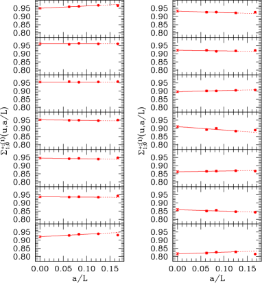
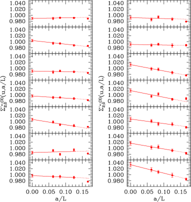
Figure 1: Continuum limit extrapolation of the SSFs $\Sigma_{1}$ (with $s=1,\,\alpha=0$) and $\Sigma_{2}$ (with $s=3,\,\alpha=0$) at various SF renormalized couplings computed using the HYP2 lattice discretisations of the static action. The SF coupling $u$ increases from top-left to bottom-right.

The maximal statistical uncertainty for $\sigma_{k}$ is $\sim 1.5\%$ and is found at the largest value of $u$ when discarding data at $L/a=6$. The values of $\rho$ obtained in the fits of ${\cal Q}^{\prime}_{1}$ are always compatible with zero within the statistical uncertainty, while in the case of ${\cal Q}^{\prime}_{2}$ they are not compatible with zero for $u\gtrsim 2$, thus signalling a stronger dependence upon the cut-off.

6 Non-perturbative RG running in the continuum limit

In order to compute the RG running of the operators in the continuum limit as described in section 4, we need to fit the results for $\sigma_{k}(u)$ to some functional form. We follow the same procedure as for the renormalized quark mass [12], i.e. we adopt the polynomial ansatz

$$\sigma_{k}(u)=1+\sum_{m=1}^{M}s_{m}u^{m}\ ,$$ (26)

with $M=2,3,4$ and $s_{1}$ always ($s_{2}$ possibly) set to its perturbative value

$$s_{1}={\gamma}_{k}^{\prime(0)}\ln 2\ ,\qquad\qquad s_{2}=\gamma_{k}^{\prime(1)}\ln 2+\left[\frac{1}{2}(\gamma_{k}^{\prime(0)})^{2}+b_{0}\gamma_{k}^{\prime(0)}\right](\ln 2)^{2}\ .$$ (27)

It is worth mentioning that if $s_{2}$ is fitted as a free parameter, it turns out to lie in the ballpark of perturbation theory. The RG running factor ${\hat{c}}^{\prime}_{k}(\mu_{\rm had})={\hat{c}}^{\prime}_{k}(2^{n}\mu_{\rm had})U^{\prime}_{k}(2^{n}\mu_{\rm had},\mu_{\rm had})$, which is now a function of the fit parameters only, can be obtained with a complete control of the systematic effects. We have indeed checked that its value is fairly insensitive to the fit ansatz and to whether $s_{2}$ is set to its perturbative value or not. We choose to quote as our final results those obtained with $M=3$, $s_{1}$ fixed by perturbation theory and $s_{2}$, $s_{3}$ kept as free parameters. In practice, due to constrains imposed by Heavy Quark Spin Symmetry, the number of independent SF schemes for ${\cal Q}^{\prime}_{k}$ is downgraded to four for $k=1$ and to eight for $k=2$. These lead to total RGI renormalization factors which are scheme independent apart from ${\rm O}(a)$ lattice artefacts. The main criterion to define suitable schemes amounts to checking that the systematic uncertainty related to truncating the perturbative evolution factor ${\hat{c}}^{\prime}_{k}(\mu_{\rm pt})$ of Eq. (20) at NLO in the anomalous dimension is well under control. This in turn requires an estimate of the size of the NNLO contribution to ${\hat{c}}^{\prime}_{k}(\mu_{\rm pt})$. To this purpose we have re-computed ${\hat{c}}^{\prime}_{k}(\mu_{\rm pt})$ with two different values of the NNLO anomalous dimensions $\gamma_{k}^{\prime(2)}$: in the first case we set $|\gamma_{k}^{\prime(2)}/\gamma_{k}^{\prime(1)}|=|\gamma_{k}^{\prime(1)}/\gamma_{k}^{\prime(0)}|$; in the second case, we guess $\gamma_{k}^{\prime(2)}$ by performing a one-parameter fit to the SSF with $s_{1},s_{2}$ fixed by perturbation theory, and equating the resulting value of $s_{3}$ to its perturbative expression

$$s_{3}=\gamma_{k}^{\prime(2)}\ln 2 +\left[\gamma_{k}^{\prime(0)}\gamma_{k}^{\prime(1)}+2b_{0}\gamma_{k}^{\prime(1)}+b_{1}\gamma_{k}^{\prime(0)}\right](\ln 2)^{2}+$$ (28)

$$+\left[\frac{1}{6}(\gamma_{k}^{\prime(0)})^{3}+b_{0}(\gamma_{k}^{\prime(0)})^{2}+\frac{4}{3}b_{0}^{2}\gamma_{k}^{\prime(0)}\right](\ln 2)^{3}\,.$$

For the operator ${\cal Q}^{\prime}_{1}$, we find that in either case the central value of the combination ${\hat{c}}^{\prime}_{k}(\mu_{\rm had})\equiv{\hat{c}}^{\prime}_{k}(\mu_{\rm pt})U^{\prime}_{k}(\mu_{\rm pt},\mu_{\rm had})$ changes by a small fraction of the statistical error, of the order $0.1$–$0.3$ standard deviations (depending on the renormalization scheme). For the operator ${\cal Q}^{\prime}_{2}$, which carries relatively large NLO anomalous dimensions, the effect can be as large as $0.8$–$1.0$ standard deviations. Therefore, we add to ${\hat{c}}^{\prime}_{2}(\mu_{\rm had})$ a corresponding systematic uncertainty of this order. It has to be stressed that the impact of this extra uncertainty at the level of the $B$–$\bar{B}$ mixing amplitude is not particularly worrying, since the matrix element of ${\cal Q}^{\prime}_{2}$ enters the latter only at ${\rm O}(\alpha_{s})$, when the static-light theory is matched to QCD. The results for the SSFs and the operator RG running in the reference schemes (see the end of Section 3) are illustrated in Figure 2.

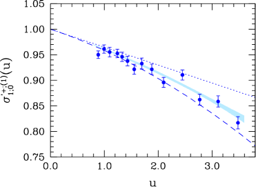
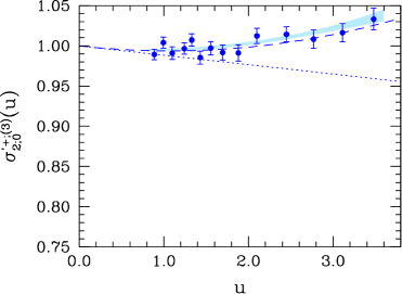
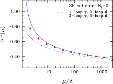
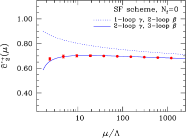
Figure 2: Upper plots: the step scaling functions $\sigma_{12}$ (discrete points) as obtained non-perturbatively. The shaded area is the one sigma band obtained by fitting the points to a polynomial. The dotted (dashed) line is the LO (NLO) perturbative result. Lower plots: RG running of ${\cal Q}^{\prime}_{1,2}$ obtained non perturbatively (discrete points) at specific values of the renormalization scale $\mu$, in units of $\Lambda$. The lines are perturbative results at the order shown for the Callan-Symanzik $\beta$-function and the operator anomalous dimension $\gamma$.

7 Matching to hadronic observables

The RGI operator is connected to its bare counterpart via the total renormalization factor ${\hat{Z}}^{\prime}_{k,\rm RGI}(g_{0})$ of Eq. (24). We stress that ${\hat{Z}}^{\prime}_{k,\rm RGI}(g_{0})$ is a scale-independent quantity, which moreover depends upon the renormalization scheme only via cutoff effects. Indeed, it depends on the particular lattice regularization chosen, though only via the factor ${\hat{\cal Z}}^{\prime}_{k}(g_{0},a\mu_{\rm had})$, the computation of which is much less expensive than the total RG running factor ${\hat{c}}^{\prime}_{k}(\mu_{\rm had})$.

We have computed ${\cal Z}^{\prime}_{k}(g_{0},a\mu_{\rm had}),\,\mu_{\rm{had}}=1/(2L_{\rm max})$ non-perturbatively at four values of $\beta$ for each scheme and four-fermion operator, and for the four different static actions under consideration. The total renormalization factors are obtained upon multiplying by the corresponding running factors on third column of Table 1. Polynomial interpolations of the form

$${\hat{Z}}^{\prime}_{k,\rm RGI}(g_{0})=a_{k}+b_{k}(\beta-6)+c_{k}(\beta-6)^{2}\ ,$$ (29)

can be subsequently used to obtain the total renormalization factor at any value of $\beta$ within the covered range $(6.0\leq\beta\leq 6.5)$. We provide in Table 1 the resulting fit coefficients for the HYP2 action in our reference renormalization schemes. These parametrizations represent our data with an accuracy of at least $0.3\%$. The contribution from the error in the RG running factors of Table 1 has not been included: since these factors have been computed in the continuum limit, they should be added in quadrature after the quantity renormalized with the factor derived from Eq. (29) has been extrapolated itself to the continuum limit.

$k$	$s$	${\hat{c}}^{\prime}_{k}(\mu_{\rm had})$	$~{}~{}~{}~{}a_{k}$	$~{}~{}~{}~{}b_{k}$	$~{}~{}~{}c_{k}$
1	1	0.777(17)	0.5731(11)	-0.171(11)	0.082(25)
2	3	0.675(12)	0.7258(14)	-0.061(14)	0.016(33)

Table 1: Running ${\hat{c}}^{\prime}_{k}(\mu_{\rm had})$ (with $\mu_{\rm had}=(2L_{\rm max})^{-1}$) and fits to the total renormalization factor of Eq. 24.

8 SF correlators for the bare matrix elements

In order to simulate the physical matrix elements needed for the $B$-parameter, we adopt a formalism similar to the one described in the previous sections, where the heavy quark field is described by the HYP2 static action, while the light quark field is described by the tmQCD action including the Sheikoleslami-Wohlert term with non-perturbatively defined $c_{\rm sw}$. The interpolating operators of the $B_{s}$- and $\bar{B}_{s}$-mesons are provided by the boundary sources $\Sigma_{sh}$ and $\Sigma^{\prime}_{s\bar{h}}$. Correlation functions are then constructed by inserting a bilinear or a four-fermion operator in the bulk of the SF. Accordingly, the building blocks of the computation are given by

$$f_{\rm\scriptscriptstyle X}(x_{0})=-\frac{\ a^{3}}{\ 2\ }\sum_{\mathbf{x}}\langle X_{hs}(x)\Sigma_{sh}\rangle\ ,\qquad f^{\prime}_{\rm\scriptscriptstyle X}(x_{0})=-\frac{\ a^{3}}{\ 2\ }\sum_{\mathbf{x}}\langle\Sigma^{\prime}_{s\bar{h}}X_{\bar{h}s}(x)\rangle\ ,$$ (30)

$$F_{\rm\scriptscriptstyle Y}(x_{0})=a^{3}\sum_{\mathbf{x}}\langle\Sigma^{\prime}_{s\bar{h}}Y_{hs\bar{h}s}(x)\Sigma_{sh}\rangle\ ,$$ (31)

where $X=A_{0}^{\rm stat},V_{0}^{\rm stat}$ and $Y={\cal Q}^{\prime}_{1,2}$. To be precise, the extraction of the $B$-parameter of Eq. (1) requires that the matrix elements of ${\cal Q}^{\prime}_{1,2}$ be normalized by the square of the decay matrix element of the $B_{s}$-meson mediated by the static axial current. Since the latter is rotated at full twist into a linear combination of axial and vector currents, we obtain the single contributions to the $B$-parameter from the plateau region of the ratios

$$R_{i}(x_{0})=\frac{3}{8}\frac{F_{\scriptscriptstyle{\cal Q}^{\prime}_{i}}(x_{0})}{[2h_{\rm\scriptscriptstyle A-iV}(x_{0})][2h^{\prime}_{\rm\scriptscriptstyle A-iV}(T-x_{0})]}\ ,\qquad i=1,2\ ,$$ (32)

where

$$h_{\rm\scriptscriptstyle A-iV}(x_{0})=\frac{1}{\sqrt{2}}\left[Z^{\rm stat}_{\rm\scriptscriptstyle A,RGI}f_{\rm\scriptscriptstyle A}^{\rm stat}(x_{0})-Z^{\rm stat}_{\rm\scriptscriptstyle V,RGI}f_{\rm\scriptscriptstyle V}^{\rm stat}(x_{0})\right]\ .$$ (33)

The RGI axial constant $Z^{\rm stat}_{\rm\scriptscriptstyle A,RGI}$ has been non-perturbatively computed in [14, 9]. The scale independent ratio $Z^{\rm stat}_{\rm\scriptscriptstyle V,RGI}/Z^{\rm stat}_{\rm\scriptscriptstyle A,RGI}$ is taken from [15]. We performed simulations at $\beta=6.0,6.1,6.2$ with the strange quark mass set to physical values as in [16]. Lattice parameters are collected in Table 2.

9 Analysis of the excited state contaminations

The standard way to identify a plateau interval for a three-point correlation function such as Eq. (31) is to analyse the exponential decay rate of the corresponding meson propagator $h_{\rm\scriptscriptstyle A-iV}$, obtained via the binding energy

$\beta$	$T\times L^{3}$	$\kappa_{\rm cr}$	$\kappa$	$\mu$
$6.0$	$32\times 16^{3}$	$0.135196$	$0.135181$	$0.028669$
$6.1$	$38\times 24^{3}$	$0.135665$	$0.135650$	$0.028532$
$6.2$	$44\times 24^{3}$	$0.135795$	$0.135785$	$0.022890$

Table 2: Lattice parameters

$$aE_{\rm eff}(x_{0})=\frac{1}{2}\log\left\{\frac{h_{\rm\scriptscriptstyle A-iV}(x_{0}-a)}{h_{\rm\scriptscriptstyle A-iV}(x_{0}+a)}\right\}\ .$$ (34)

This procedure may work only provided that the lowest value $x_{0}^{\rm min}$, at which the fundamental state is numerically isolated, fulfills the condition $x_{0}^{\rm min}<T/2$. Correspondingly, the interval $[x_{0}^{\rm min},T-x_{0}^{\rm min}]$ can be certainly used to extract the plateau value of the three-point correlator. Unfortunately, this is not the case, as shown in Figs. 3 and 4 (left): due to the small mass gap between the lowest and the first excited states in the static-light channel, the plateau starts at about the middle of the lattice. Simulations at larger time extensions are increasingly expensive owing to the exponential rise of the noise-to-signal ratio related to static propagators.

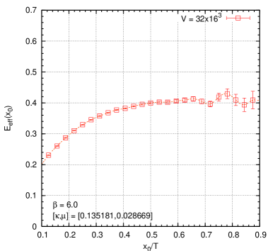
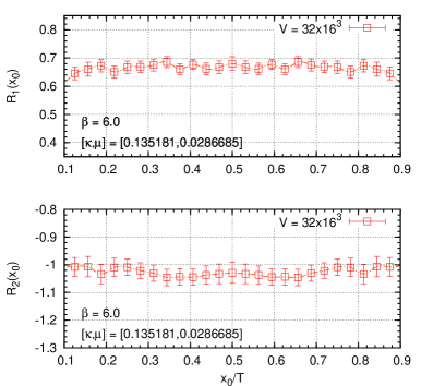
Figure 3: The binding energy and the contributions to the $B_{s}$-parameter at $\beta=6.0$.

Irrespective of this, the observables $R_{i}$ are characterized by a very flat time dependence; examples are provided by Figs. 3 and 4 (right). In order to understand this behaviour, we perform an expansion of Eqs. (30,31) through the insertion of complete sets of Hamiltonian eigenstates. Assuming that the excited contributions in the vacuum channel may be disregarded, one easily arrives at the representation

$$R_{i}(x_{0})=B_{i}^{(0,0)}\frac{1+\sum_{(n,m)\neq(0,0)}^{\infty}\frac{B_{i}^{(n,m)}}{B_{i}^{(0,0)}}f_{nm}g_{nm}{\rm e}^{-(T-x_{0})\Delta^{(B)}_{n0}}{\rm e}^{-x_{0}\Delta^{(B)}_{n0}}}{1+\sum_{(n,m)\neq(0,0)}^{\infty}\ \ \ \ \ \ \ f_{nm}g_{nm}{\rm e}^{-(T-x_{0})\Delta^{(B)}_{n0}}{\rm e}^{-x_{0}\Delta^{(B)}_{n0}}}\ ,$$ (35)

where $\Delta^{(B)}_{n0}=E^{(B)}_{n}-E^{(B)}_{0}$ is the energy gap between the $n$-th Hamiltonian eigenstate $|n,B\rangle$ with the quantum numbers of a static $B_{s}$-meson and the fundamental state. Moreover,

$$B_{i}^{(n,m)}=\frac{\langle n,B|{\cal Q}^{\prime}_{i}|m,B\rangle}{\frac{8}{3}\langle n,B|A_{0}|0,0\rangle\langle 0,0|A_{0}|m,B\rangle}\ ,$$ (36)

$$f_{nm}=\frac{\langle{\rm i}_{B}|n,B\rangle\langle m,B|{\rm i}_{B}\rangle}{\langle{\rm i}_{B}|0,B\rangle\langle 0,B|{\rm i}_{B}\rangle}\ ,\qquad g_{nm}=\frac{\langle n,B|A_{0}|0,0\rangle\langle 0,0|A_{0}|m,B\rangle}{\langle 0,B|A_{0}|0,0\rangle\langle 0,0|A_{0}|0,B\rangle}\ .$$ (37)

Here $|{\rm i}_{B}\rangle$ represents the SF boundary state corresponding to the action of the bilinear sources Eq. (10) on the vacuum. In particular, one should observe that $B_{i}^{(n,m)}$ represents a generalization of the $B$-parameter, describing the particle-antiparticle mixing of excited states. Numerator and denominator of Eq. (35) look quite similar. They only differ by the weighting coefficients $z_{nm}=B_{i}^{(n,m)}/B_{i}^{(0,0)}$.

The hypothetical condition $z_{nm}\approx 1$ would act on the ratios $R_{i}(x_{0})$ as an additional damping factor of the excited state contaminations, together with the exponential decays due to the mass gaps $\Delta_{nm}^{(B)}$. In practice, what really matters for our concern is the first excited contribution, because already the second excitation is reasonably expected to compete with the $0^{++}$ glueball ($r_{0}m_{G}\approx 1.7\ {\rm GeV}$). Data suggest that $z_{10}$ could be quite close to one.

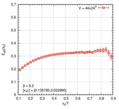
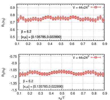
Figure 4: The binding energy and the contributions to the $B_{s}$-parameter at $\beta=6.2$.

Since the quantum states $|B,n\rangle$ and $|B,0\rangle$ differ only by their mass, we are led to speculate about the mass dependence of the generalized $B$-parameters $B^{(n,m)}_{i}$. Although quantitative statements are highly non-trivial, it is not difficult to identify at least one extreme situation where the limits $z_{nm}=1$ could be realized. This is a scenario in which $B_{i}^{(n,m)}$ is weakly dependent upon the mass of the external states. If $B_{i}^{(n,m)}$ is close to $B_{i}^{(0,0)}$, then their ratio will be close to one. This picture imposes no restrictions on the value of $B_{i}^{(0,0)}$.

An apparently different possibility is represented by the VSA, which implies $B_{i}^{(n,m)}=1$, and consequently $z_{nm}=1$. Though speculative, it is not unreasonable that the violation of the VSA depends weakly upon the mass of the external states and is responsible in the end for the realization of the above-mentioned scenario.

A quantitative check of the suppression of excited state contaminations in $R_{1,2}(x_{0})$ would be provided by the level of stability of the observed plateaux under a variation of the boundary interpolating operators. In the framework of the Schrödinger functional this possibility is explored via the introduction of boundary wave functions like in [17]. Unfortunately, the computational price required at present for the practical implementation of this smearing technique amounts to giving up one of the boundary summations of Eq. (10), with a corresponding increase of the statistical error by a factor of $\sqrt{L^{3}}$. The situation is even worse with a three-point correlator such as Eq. (31), which has interpolating sources on both boundaries. In this case the introduction of smearing wave functions increases the statistical noise by a factor of $L^{3}$, which makes the check useless. This problem can be hopefully overcome through the implementation of a SF all-to-all propagator like proposed in [18, 19, 20]. This is currently under way.

10 A two-state stochastic model

In order to have a qualitative view about the impact of large deviations of $z_{10}$ from one on the time dependence of $R_{i}(x_{0})$, we consider a two-state model. Here, the binding energy and the contributions to the $B$-parameters are described by the stochastic variables

$$\epsilon(e,x_{0},T) =e+\frac{1}{2}\log\left\{\frac{1-p{\rm e}^{-\Delta(x_{0}-1)}}{1-p{\rm e}^{-\Delta(x_{0}+1)}}\right\}\ ,$$ (38)

$$\rho(z,x_{0},T) =\frac{1-zp\left[{\rm e}^{-\Delta(x_{0})}+{\rm e}^{-\Delta(T-x_{0})}\right]}{1-p\left[{\rm e}^{-\Delta(x_{0})}+{\rm e}^{-\Delta(T-x_{0})}\right]}\ ,$$ (39)

where $p$ and $\Delta$ are differently distributed random coefficients, while $z$ and $e$ parametrize $z_{10}$ and $E_{0}^{(B)}$. Obviously, $\Delta$ is meant to represent the energy gap of the first excited state. From a two-state analysis of $E_{\rm eff}(x_{0})$, it is roughly known that $a\Delta\approx 0.22(3)$. Therefore, we model this variable according to a Gaussian distribution probability, i.e.

$$P(\Delta)=\frac{1}{\sigma_{\Delta}\sqrt{2\pi}}{\rm exp}\left(-\frac{\Delta-\bar{\Delta}}{2\sigma_{\Delta}^{2}}\right)\ ,\qquad(\bar{\Delta},\sigma_{\Delta})=(0.22,0.03)\ .$$ (40)

On the other hand, $p$ is supposed to represent the product of the matrix elements $f_{10}$ and $g_{10}$, defined in Eq. (37). Choosing a distribution probability for this variable is delicate, because we are largely ignorant about the projection of the SF boundary state $|{\rm i}_{B}\rangle$ onto the first excited state $|1,B\rangle$ and the decay constant of the latter. We can heuristically expect that

$$h_{10}=\frac{\langle 1,B|A_{0}|0,0\rangle}{\langle 0,B|A_{0}|0,0\rangle}=\frac{m_{B}^{*}f_{B}^{*}}{m_{B}f_{B}}\approx 1\ .$$ (41)

Nevertheless, if we believe that $|{\rm i}_{B}\rangle$ is well projected onto $|0,B\rangle$, then $f_{10}\approx 0$. In this case we should choose a probability distribution of $p$ peaked around $p=0$. By contrast, if we believe that $|{\rm i}_{B}\rangle$ is a balanced mixture of $|0,B\rangle$ and $|1,B\rangle$, it follows that $f_{10}\approx 1$. It makes sense to assume a given sign for $p$ and not to allow for fluctuations of the opposite sign. A flexible distribution probability allowing for a definite sign is the Log-normal distribution, defined by

$$P(p;\bar{p},\sigma_{p})=\frac{1}{p\sigma_{p}\sqrt{2\pi}}\exp\left\{-\frac{(\ln p-\bar{p})^{2}}{2\sigma_{p}^{2}}\right\}\ .$$ (42)

Having produced $N$ samples $\{\Delta_{i}\}_{i=1\dots N}$ and $\{p_{i}\}_{i=1\dots N}$ of $\Delta$ and $p$, we approximate the ensemble averages of $\mu(z,x_{0},T)$ and $\epsilon(e,x_{0},T)$ via

$${\cal E}(e,x_{0},T) =\langle\epsilon(e,x_{0},T)\rangle\simeq e+\frac{1}{2N}\sum_{i=1}^{N}\log\left\{\frac{1-p_{i}{\rm e}^{-\Delta_{i}(x_{0}-1)}}{1-p{\rm e}^{-\Delta_{i}(x_{0}+1)}}\right\}\ ,$$ (43)

$${\cal R}(z,x_{0},T) =\langle\rho(z,x_{0},T)\rangle\simeq\frac{1}{N}\sum_{i=1}^{N}\frac{1-zp_{i}\left[{\rm e}^{-\Delta_{i}(x_{0})}+{\rm e}^{-\Delta_{i}(T-x_{0})}\right]}{1-p_{i}\left[{\rm e}^{-\Delta_{i}(x_{0})}+{\rm e}^{-\Delta_{i}(T-x_{0})}\right]}\ .$$ (44)

The ensemble averages $\cal E$ and $\cal R$ are now functions of the distribution parameters $\bar{p}$ and $\sigma_{p}$, which can be varied in order to change the shape of the distribution. One of the worst cases we considered is the one corresponding to $(\bar{p}=-1/8,\sigma_{p}=1/4)$, i.e a Log-normal distribution peaked around $\exp(-\bar{p})\simeq 0.88$. In the spirit of the two-state model, such a distribution describes a large overlap between the interpolating boundary state and the first excited one. As shown in Fig. 5, the binding energy resembles very closely the one of Fig. 3. The shapes of the $B$-parameter corresponding of different choices of $z$ suggest that $z_{10}$ could be very close to one in the real case, thus supporting our interpretation in terms of the VSA.

11 Conclusions

$B^{0}-\bar{B}^{0}$ mixing remains among the most important processes that are required to pin down the elements of the CKM matrix precisely. However, in order to constrain the unitarity triangle sufficiently well and to look for signs of new physics, theoretical uncertainties associated with hadronic effects must be reduced. In this talk we have reported on a new strategy for the computation of the heavy-light $B$-parameters in lattice QCD, based on tmQCD and HQET. Its main advantage is the exact absence of mixing under renormalization, which plagues standard Wilson fermions, at the same computational cost of a Wilson-type regularization. We have described our fully non-perturbative calculation of the relations between parity-odd, static-light four-quark operators in quenched lattice QCD and their renormalized counterparts. We have also described our first experiences with the computation of the bare matrix elements for the $B_{s}-\bar{B}_{s}$ mixing and their excited state contaminations. Before attempting a continuum extrapolation of the matrix elements, a deeper analysis of the excited state contributions has to be done and we hope that the all-to-all propagator, like proposed in [18, 19, 20] will be of great help there.

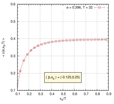
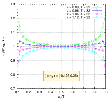
Figure 5: The binding energy and the contributions to the $B_{s}$-parameter within a two-state stochastic model.

References

-
[1]
R. Frezzotti, P. A. Grassi, S. Sint and P. Weisz,
JHEP 0108 (2001) 058
[arXiv:hep-lat/0101001].
- [2] G. Buchalla, Phys. Lett. B 395 (1997) 364 [arXiv:hep-ph/9608232].
- [3] F. Palombi, M. Papinutto, C. Pena and H. Wittig, JHEP 0608 (2006) 017 [arXiv:hep-lat/0604014].
- [4] F. Palombi, M. Papinutto, C. Pena and H. Wittig, arXiv:0706.4153 [hep-lat].
- [5] M. Lüscher, R. Narayanan, P. Weisz and U. Wolff, Nucl. Phys. B 384 (1992) 168 [arXiv:hep-lat/9207009].
- [6] P. Dimopoulos, G. Herdoiza, F. Palombi, M. Papinutto, C. Pena, A. Vladikas and H. Wittig, PoS(LAT2007)368 arXiv:0710.2862 [hep-lat].
- [7] M. Luscher, S. Sint, R. Sommer and P. Weisz, Nucl. Phys. B 478 (1996) 365 [arXiv:hep-lat/9605038].
- [8] E. Eichten and B. R. Hill, Phys. Lett. B 234 (1990) 511.
- [9] M. Della Morte, A. Shindler and R. Sommer, JHEP 0508 (2005) 051 [arXiv:hep-lat/0506008].
- [10] S. Necco and R. Sommer, Phys. Lett. B 523 (2001) 135 [arXiv:hep-ph/0109093].
- [11] A. Bode, P. Weisz and U. Wolff, Nucl. Phys. B 576 (2000) 517 [Erratum-ibid. B 600 (2001 ERRAT,B608,481.2001) 453] [arXiv:hep-lat/9911018].
- [12] S. Capitani, M. Lüscher, R. Sommer and H. Wittig, Nucl. Phys. B 544 (1999) 669 [arXiv:hep-lat/9810063].
- [13] A. Hasenfratz and F. Knechtli, Phys. Rev. D 64 (2001) 034504 [arXiv:hep-lat/0103029].
- [14] J. Heitger, M. Kurth and R. Sommer, Nucl. Phys. B 669 (2003) 173 [arXiv:hep-lat/0302019].
- [15] F. Palombi, arXiv:0706.2460 [hep-lat].
- [16] J. Rolf and S. Sint, JHEP 0212 (2002) 007 [arXiv:hep-ph/0209255].
- [17] M. Della Morte, S. Dürr, J. Heitger, H. Molke, J. Rolf, A. Shindler and R. Sommer, Phys. Lett. B 581 (2004) 93 [Erratum-ibid. B 612 (2005) 313] [arXiv:hep-lat/0307021].
- [18] L. Giusti, P. Hernandez, M. Laine, P. Weisz and H. Wittig, JHEP 0404 (2004) 013 [arXiv:hep-lat/0402002].
- [19] J. Foley, K. Jimmy Juge, A. O’Cais, M. Peardon, S. M. Ryan and J. I. Skullerud, Comput. Phys. Commun. 172 (2005) 145 [arXiv:hep-lat/0505023].
- [20] M. Lüscher, JHEP 0707 (2007) 081 arXiv:0706.2298 [hep-lat].