Non-perturbative renormalisation of four-fermion operators in $N_{\mathrm{\scriptstyle f}}=2$ QCD

Abstract:

We present results for the non-perturbative renormalisation of four-fermion operators with two flavours of dynamical quarks. We consider both fully relativistic left current-left current operators, and a full basis for $\Delta B=2$ operators with static heavy quarks. The renormalisation group running of the operators to high energy scales is computed in the continuum limit for a family of Schrödinger Functional renormalisation schemes, via standard finite size scaling techniques. The total renormalisation factors relating renormalisation group invariant to bare operators are computed for a choice of lattice regularisations.

1 Introduction

Hadronic matrix elements (HMEs) of four-fermion operators have long been essential input quantities for Flavour Physics. Reliable estimates of a number of HMEs are crucial in the study of CP violation via CKM unitarity triangle analyses, or of such striking experimental findings as the enhancement of hadronic decay amplitudes by long-distance effects (as e.g. in the $\Delta I=1/2$ rule). The only known technique to compute HMEs from first principles is lattice QCD. However, lattice QCD results have long been hampered by the difficulty to eliminate a number of systematic uncertainties. Most notably, the high cost of including dynamical quark effects in lattice QCD simulations has enforced for many years either the quenched approximation, or the use of dynamical quark masses far too heavy to allow for a well-controlled extrapolation to the physical regime. In some cases, e.g. the computation of the kaon bag parameter $B_{K}$, quenching effects are indeed the last remaining uncontrolled systematic uncertainty [1].

As techniques for the simulation of light dynamical quarks have witnessed dramatic progress in the last few years (see e.g. [2]), it becomes increasingly important to bring to this environment the techniques to control other sources of uncertainty, in order to aim at precision computations of physical quantities. In the context of HMEs, one of the most prominent examples is non-perturbative renormalisation (NPR) (see e.g. [3]). The use of finite-size scaling techniques has allowed to control fully both the renormalisation group (RG) running and the matching of lattice to renormalised observables in the quenched approximation for a broad class of four-fermion operators [4, 5, 6]. The aim of the present work is to extend these results to $N_{\mathrm{\scriptstyle f}}=2$ QCD. In particular, we will discuss 1. the RG running of left current-left current relativistic four-fermion operators, 2. the RG running of all $\Delta B=2$ operators with static heavy quarks, and 3. the matching of the above operators to renormalised continuum operators for some particular choices of the regularisation. Immediate applications, as we will point out later, arise in the computation of the bag parameters $B_{K}$ and $B_{B}$. Preliminary results had been presented at last year’s conference [7].

2 Definitions and setup

2.1 Renormalisation of four-fermion operators

We will consider two different classes of operators:

$$O^{\pm}_{\Gamma_{1},\Gamma_{2}}(x) =\frac{1}{2}\left[\left(\bar{\psi}_{1}(x)\Gamma_{1}\psi_{2}(x)\right)\left(\bar{\psi}_{3}(x)\Gamma_{2}\psi_{4}(x)\right)\pm(2\leftrightarrow 4)\right]\,,$$ (1)

$${\cal O}^{\pm}_{\Gamma_{1},\Gamma_{2}}(x) =\frac{1}{2}\left[\left(\bar{\psi}_{h}(x)\Gamma_{1}\psi_{2}(x)\right)\left(\bar{\psi}_{\bar{h}}(x)\Gamma_{2}\psi_{4}(x)\right)\pm(2\leftrightarrow 4)\right]\,.$$ (2)

In the above expressions $\psi_{k}$ is a relativistic quark field with flavour index $k$, $\psi_{h,\bar{h}}$ are static (anti)quark fields, $\Gamma_{l}$ are spin matrices, and the parentheses indicate spin-colour traces. All the fields are interpreted to be in the valence sector of the theory. This formalism of distinct quark flavours will allow us to isolate scale-dependent logarithmic divergences from eventual mixing with lower-dimensional operators that may appear for specific choices of quark masses and/or flavour content.

The above operators mix under renormalisation as determined by the symmetries of the regularised theory. If we restrict ourselves to the parity-odd sector, complete bases of operators in the relativistic and static cases are given by

$$Q^{\pm}_{k}\in\left\{O^{\pm}_{\rm\scriptscriptstyle VA+AV},O^{\pm}_{\rm\scriptscriptstyle VA-AV},O^{\pm}_{\rm\scriptscriptstyle SP-PS},O^{\pm}_{\rm\scriptscriptstyle SP+PS},O^{\pm}_{\rm\scriptscriptstyle T\tilde{T}},\right\}\,;~{}~{}~{}~{}~{}{\cal Q}^{\pm}_{k}\in\left\{{\cal O}^{\pm}_{\rm\scriptscriptstyle VA+AV},{\cal O}^{\pm}_{\rm\scriptscriptstyle VA-AV},{\cal O}^{\pm}_{\rm\scriptscriptstyle SP-PS},{\cal O}^{\pm}_{\rm\scriptscriptstyle SP+PS},\right\}\,,$$ (3)

respectively, in standard self-explanatory notation for the choice of spin matrices $\Gamma_{l}$. A full analysis of the renormalisation of these operator bases with relativistic Wilson fermions has been performed in [8, 9]. One particular conclusion is that, contrary to the parity-even case, discrete symmetries protect all the above operators from extra mixings under renormalisation due to the breaking of chiral symmetry. Recall that the RG of these operators and of their parity-even partners is identical, as in the continuum limit (CL) chiral symmetry holds. On the other hand, the connection to observables involving matrix elements of parity-even operators is non-trivial.

From now on, we will consider the subset of operators

$$Q_{1}^{\pm}\,,~{}~{}{\cal Q}^{{}^{\prime}+}_{k}\in\left\{{\cal Q}^{+}_{1},{\cal Q}^{+}_{1}+4{\cal Q}^{+}_{2},{\cal Q}^{+}_{3}+2{\cal Q}^{+}_{4},{\cal Q}^{+}_{3}-2{\cal Q}^{+}_{4}\right\}\,.$$ (4)

All these operators renormalise multiplicatively — i.e., given an operator $O\in\{Q_{1}^{\pm},{\cal Q}^{{}^{\prime}+}_{k}\}$ the corresponding operator insertion in any on-shell renormalised correlation function is given by

$$O_{\rm R}(x;\mu)=\lim_{a\to 0}Z(g_{0},a\mu)\,O(x;g_{0})\,,$$ (5)

where $g_{0},a$ are the bare lattice coupling and the lattice spacing, respectively. The RG running of the operator is controlled by the anomalous dimension $\gamma$, defined by the Callan-Symanzik equation

$$\mu\frac{\partial}{\partial\mu}O_{\rm R}(x;\mu)=\gamma(\kern 1.0pt\overline{\kern-1.0ptg\kern 0.0pt}\kern 1.0pt(\mu))\,O_{\rm R}(x;\mu)\,,$$ (6)

which is supplemented by the corresponding Callan-Symanzik equation for the renormalised coupling

$$\mu\frac{\partial}{\partial\mu}\kern 1.0pt\overline{\kern-1.0ptg\kern 0.0pt}\kern 1.0pt(\mu)=\beta(\kern 1.0pt\overline{\kern-1.0ptg\kern 0.0pt}\kern 1.0pt(\mu))\,.$$ (7)

In mass-independent renormalisation schemes, the beta function and all anomalous dimensions do indeed depend only on the renormalised coupling $\kern 1.0pt\overline{\kern-1.0ptg\kern 0.0pt}\kern 1.0pt$. They admit perturbative expansions of the form

$$\beta(g)\stackrel{{\scriptstyle g\to 0}}{{\approx}}-g^{3}\left(b_{0}+b_{1}g^{2}+b_{2}g^{4}+\ldots\right)\,;~{}~{}~{}~{}~{}~{}~{}\gamma(g)\stackrel{{\scriptstyle g\to 0}}{{\approx}}-g^{2}\left(\gamma_{0}+\gamma_{1}g^{2}+\gamma_{2}g^{4}+\ldots\right)\,,$$ (8)

in which the coefficients $b_{0},b_{1},\gamma_{0}$ are renormalisation scheme-independent. Upon formal integration of Eq. (6), one is left with the renormalisation group invariant (RGI) operator insertion

$$\hat{O}(x)=O_{\rm R}(x;\mu)\,\left[\frac{\kern 1.0pt\overline{\kern-1.0ptg\kern 0.0pt}\kern 1.0pt^{2}(\mu)}{4\pi}\right]^{-\frac{\gamma_{0}}{2b_{0}}}\exp\left\{-\int_{0}^{\kern 1.0pt\overline{\kern-1.0ptg\kern 0.0pt}\kern 1.0pt(\mu)}{\rm d}g\,\left(\frac{\gamma(g)}{\beta(g)}-\frac{\gamma_{0}}{b_{0}g}\right)\right\}\,,$$ (9)

while the RG evolution between two scales $\mu_{1},\mu_{2}$ is given by the operator

$$U(\mu_{2},\mu_{1})=\exp\left\{\int_{\kern 1.0pt\overline{\kern-1.0ptg\kern 0.0pt}\kern 1.0pt(\mu_{1})}^{\kern 1.0pt\overline{\kern-1.0ptg\kern 0.0pt}\kern 1.0pt(\mu_{2})}{\rm d}g\,\frac{\gamma(g)}{\beta(g)}\right\}=\lim_{a\to 0}\,\frac{Z(g_{0},a\mu_{2})}{Z(g_{0},a\mu_{1})}\,.$$ (10)

2.2 Schrödinger Functional renormalisation schemes

Eq. (10) is the starting point to compute non-perturbatively the RG evolution of composite operators. To that purpose we introduce a family of Schrödinger Functional (SF) renormalisation schemes. The latter are defined by regularising the theory on a symmetric lattice of physical size $L^{4}$ with SF boundary conditions (see e.g. [10] for an introduction to the SF setup). The renormalisation scale is set to be the infrared cutoff, i.e. $\mu=1/L$. Renormalisation conditions for relativistic operators have the form

$$Z(g_{0},a\mu)\,\frac{F(x_{0})}{\Theta}=\left.\frac{F(x_{0})}{\Theta}\right|_{\rm tree~{}level}\,,$$ (11)

and are imposed in the chiral limit. In the above expression, $F$ is a four-point correlation function of the form

$$F(x_{0})=\frac{1}{L^{3}}\langle{\cal O}_{21}[\Gamma_{A}]{\cal O}_{45}[\Gamma_{B}]Q^{\pm}_{k}(x){\cal O}^{\prime}_{53}[\Gamma_{C}]\rangle\,,$$ (12)

where ${\cal O}[\Gamma]$ are bilinear interpolating fields living on the time boundaries, and $\Theta$ is a suitable boundary-to-boundary correlation function that divides out the ultraviolet divergences associated to these bilinears. Similar renormalisation conditions to Eq. (11) are set up for static-light operators, with flavours $1$ and $3$ substituted by $h$ and $\bar{h}$. Full details are provided in [4, 5, 9]. For now it is just important to mention that the renormalisation scheme is fully determined by fixing the parameters involved in the SF boundary conditions; the point $x_{0}$ at which Eq. (11) is imposed; the Dirac matrices $\Gamma_{A,B,C}$ entering boundary bilinears ; and the normalisation factor $\Theta$. Specific schemes have been introduced in [4, 5, 9]. Here we will concentrate in the cases which have been found to be best behaved in the quenched study, namely scheme $1$ for $Q^{+}_{1}$ and scheme $8$ for $Q^{-}_{1}$ in the notation of [4, 5], and the reference schemes for static-light operators defined in [6].

A crucial observation is that all the above renormalisation schemes are mass-independent by construction, and the resulting renormalisation factors are flavour-blind. It then follows that they can be used to remove the logarithmic divergences from any four-fermion operator with the considered structure, irrespective of its specific flavour content, once eventual subtractions due to mixing with equal- or lower-dimension operators have been properly performed.

2.3 Step-scaling functions

The basic objects to study the RG evolution of composite operators non-perturbatively are the step-scaling functions (SSFs)

$$\Sigma(u,a/L)=\left.\frac{Z(g_{0},a/(2L))}{Z(g_{0},a/L)}\right|_{\kern 1.0pt\overline{\kern-1.0ptg\kern 0.0pt}\kern 1.0pt^{2}(1/L)=u}\,,$$ (13)

which can be computed at several values of the lattice spacing for fixed physical size (inverse renormalisation scale) $L$. The corresponding values of $\beta$ are indeed fixed by requiring that the renormalised SF coupling $\kern 1.0pt\overline{\kern-1.0ptg\kern 0.0pt}\kern 1.0pt^{2}$, and hence $L$, are kept constant. It is then possible CL extrapolation

$$\sigma(u)\equiv\lim_{a\to 0}\Sigma(u,a/L)=\left.U((2L)^{-1},L^{-1})\right|_{\kern 1.0pt\overline{\kern-1.0ptg\kern 0.0pt}\kern 1.0pt^{2}(1/L)=u}\,.$$ (14)

Once $\sigma(u)$ is known for several different values of the squared gauge coupling $u$, it is possible to reconstruct the RG evolution factor $U(\mu_{\rm had},\mu_{\rm pt})$ between two extreme scales $\mu_{\rm had}$, in the range of a few hundred ${\rm MeV}$, and $\mu_{\rm pt}$ in the high-energy regime. This in turn allows to compute the RGI operator of Eq. (9) in a way free from large uncontrolled systematic uncertainties. It is enough to consider the exponential on the rhs of Eq. (9) evaluated at $\mu=\mu_{\rm had}$, and split it as

$$\exp\left\{-\int_{0}^{\kern 1.0pt\overline{\kern-1.0ptg\kern 0.0pt}\kern 1.0pt(\mu_{\rm had})}{\rm d}g\,\left(\frac{\gamma(g)}{\beta(g)}-\frac{\gamma_{0}}{b_{0}g}\right)\right\}=\exp\left\{-\int_{0}^{\kern 1.0pt\overline{\kern-1.0ptg\kern 0.0pt}\kern 1.0pt(\mu_{\rm pt})}{\rm d}g\,\left(\frac{\gamma(g)}{\beta(g)}-\frac{\gamma_{0}}{b_{0}g}\right)\right\}U(\mu_{\rm pt},\mu_{\rm had})\,.$$ (15)

The second factor on the rhs is known non-perturbatively, while the first factor can be safely computed at NLO in perturbation theory, provided the scale $\mu_{\rm pt}$ is high enough so as to render NNLO effects negligible.

3 Non-perturbative computation of the RG running

SSFs have been computed using the non-perturbatively $\mbox{O}(a)$ improved Wilson action, and a HYP2 action for static quarks, at six different values of the SF coupling, corresponding to six different physical lattice lengths $L$. For each volume we have simulated at three different values of the lattice spacing, corresponding to lattices with $L/a=6,8,12$ (respectively $L/a=12,16,24$) for the computation of $Z(L)$ (resp. $Z(2L)$). We used the $N_{\mathrm{\scriptstyle f}}=2$ configurations generated by the ALPHA Collaboration for the determination of the RG running of the quark mass [11]. All the technical details concerning the dynamical simulations are discussed in the mentioned work.

As we do not implement full $\mbox{O}(a)$ improvement for four-fermion operators, the only linear cutoff effects that are removed from $\Sigma(g_{0},a/L)$ are those cancelled by the SW term in the fermion action. Therefore, we expect SSFs to approach the CL linearly in $a/L$. In practice, it is often observed that the data corresponding to $L/a=8,12$ are compatible within errors, whereas the $L/a=6$ datum, that is expected to bear the largest cutoff effect, is off. This suggests that a weighted average of the results for the two finest lattices, as considered in [11], may yield a good estimate of the CL value. However, the lack of at least one extra value of $a/L$ closer to the continuum, that would allow a more precise control of the systematics, has led us to conservatively adopt linear CL extrapolations involving all the data. It is worth remarking, though, that linear fits and weighted averages lead to compatible results within one standard deviation in most cases, as can be seen in Fig. 1. The latter illustrates the extrapolations at all values of the coupling for two selected operators. Finally, let us mention that autocorrelation times, which are included in the error estimate, increase towards the CL, leading to amplified errors in the finest lattices.

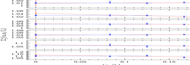
Figure 1: CL extrapolation of the SSFs for $Q_{1}^{+}$ (left) and ${\cal Q}_{1}^{{}^{\prime}+}$ (right) for one particular choice of the renormalisation scheme (all boundary matrices set to $\gamma_{5}$, spatial boundary conditions set by $\theta=0.5$, $\alpha=0$ in the renormalisation condition for ${\cal Q}_{1}^{{}^{\prime}+}$ (see [4, 5, 9] for details). The renormalised coupling increases from top to bottom and from left to right. Blue discontinued lines and the blue point at $a/L=0$ correspond to weighted averages of the $L/a=8,12$ data, red lines and the red $a/L=0$ cross to linear extrapolations in $a/L$ of the three data.

Figure 2: SSFs for $Q_{1}^{+}$ (left) and ${\cal Q}_{1}^{{}^{\prime}+}$ (right) in the CL in the same schemes as considered in Figure 1. Full red points are $N_{\mathrm{\scriptstyle f}}=2$ results, open blue points are quenched results. The red dashed (blue dotted) line is the NLO $N_{\mathrm{\scriptstyle f}}=2$ ($N_{\mathrm{\scriptstyle f}}=0$) perturbative result.

The resulting SSFs $\sigma(u)$ have been fitted to a polynomial form. For definiteness, we will provide results for a fit to $\sigma(u)=1+s_{1}u+s_{2}u^{2}+s_{3}u^{3}$, where $s_{1}$ is fixed at the value predicted by $LO$ perturbation theory and $s_{2},s_{3}$ are left as free parameters. Once this continuous form of the SSF has been obtained, it is possible to compute the relation between the RGI operators and the renormalised operators at the low-energy scale $\mu_{\rm had}=L_{\rm max}^{-1}$, defined by $\kern 1.0pt\overline{\kern-1.0ptg\kern 0.0pt}\kern 1.0pt^{2}(L_{\rm max})=4.61$, as explained e.g. in [4, 6]. This scale is chosen such that the renormalisation constant $Z(g_{0},a\mu_{\rm had})$ can be computed on accessible lattices in ranges of values of $g_{0}$ commonly used in large volume simulations. The results for the operators under investigation are reported in Table 1. Note that typical relative errors reach the 5% ballpark, which may result in a sizeable error in HMEs coming from renormalisation alone.

4 Connection to hadronic observables

RGI operator insertions can be related to bare operator insertions via a total renormalisation factor $\hat{Z}(g_{0})$, defined as

$$\hat{Z}(g_{0})=Z(g_{0},a\mu_{\rm had})\exp\left\{\int_{0}^{\kern 1.0pt\overline{\kern-1.0ptg\kern 0.0pt}\kern 1.0pt(\mu_{\rm had})}{\rm d}g\,\left(\frac{\gamma(g)}{\beta(g)}-\frac{\gamma_{0}}{b_{0}g}\right)\right\}\,.$$ (16)

This is enough to remove all ultraviolet divergences, once eventual renormalisation scale-independent mixing with operators of dimension $d\leq 6$ peculiar to the specific flavour structure under consideration has been taken into account via suitable subtractions. The details of the mixing depend on the regularisation in which bare correlation functions are computed, as does the relation between the latter and physical observables. For instance, in [12, 13] it has been explained how to extract the bag parameters $B_{K}$ and $B_{B}$ (the latter in the static limit for the $b$ quark) directly from three-point functions involving the operators $Q_{1}^{+}$ and ${\cal Q}_{1,2}^{+}$, by using Wilson actions with suitable twisted mass terms. The computation of the RGI renormalisation factors $\hat{Z}(g_{0})$ at a number of values of the bare coupling with an $\mbox{O}(a)$ improved Wilson action is under way and close to completion.

operator	ratio	operator	ratio
		${\cal Q}_{1}^{{}^{\prime};+}$	$0.724(34)$
$Q_{1}^{+}$	$1.201(66)$	${\cal Q}_{2}^{{}^{\prime};+}$	$0.647(32)$
$Q_{1}^{-}$	$0.554(21)$	${\cal Q}_{3}^{{}^{\prime};+}$	$0.539(18)$
		${\cal Q}_{4}^{{}^{\prime};+}$	$0.796(20)$

Table 1: Ratios of RGI to renormalised at $\mu_{\rm had}$ operator insertions for the various operators in the reference renormalisation schemes mentioned in the text.

5 Conclusions

We have presented a fully non-perturbative computation of the RG running of a wide class of four-fermion operators in $N_{\mathrm{\scriptstyle f}}=2$ QCD. These results, together with the matching to specific hadronic schemes, is a basic building block of any $N_{\mathrm{\scriptstyle f}}=2$ computation of such quantities as $B_{K}$ and $B_{B}$ that aims at eliminating systematic uncertainties related to renormalisation. On the other hand, the precision of the results sets a potentially unsatisfactory lower bound for the final error on weak matrix elements. Future refinement, e.g. by adding a finest lattice to our continuum limit extrapolations, can be hence desirable. These issues will be discussed in detail in our forthcoming publication of the definitive results.

References

- [1] C. Dawson, PoS LAT2005, 007 (2006); C. Pena, PoS LAT2006 (2006) 019.
- [2] L. Giusti, PoS LAT2006 (2006) 009.
- [3] R. Sommer, Nucl. Phys. Proc. Suppl. 119 (2003) 185.
- [4] M. Guagnelli et al. [ALPHA Collaboration], JHEP 0603 (2006) 088.
- [5] F. Palombi, C. Pena and S. Sint, JHEP 0603 (2006) 089.
- [6] F. Palombi, M. Papinutto, C. Pena and H. Wittig, arXiv:0706.4153 [hep-lat].
- [7] P. Dimopoulos, G. Herdoiza, A. Vladikas, F. Palombi, C. Pena and S. Sint [ALPHA Collaboration], PoS LAT2006 (2006) 158 [arXiv:hep-lat/0610077].
- [8] A. Donini et al. Eur. Phys. J. C 10, 121 (1999).
- [9] F. Palombi, M. Papinutto, C. Pena and H. Wittig, JHEP 0608 (2006) 017.
- [10] R. Sommer, arXiv:hep-lat/0611020.
- [11] M. Della Morte et al. [ALPHA Collaboration], Nucl. Phys. B 729 (2005) 117.
- [12] R. Frezzotti, P.A. Grassi, S. Sint and P. Weisz [ALPHA Collaboration], JHEP 0108, 058 (2001); P. Dimopoulos et al. [ALPHA Collaboration], Nucl. Phys. B 749 (2006) 69.
- [13] M. Della Morte, Nucl. Phys. Proc. Suppl. 140 (2005) 458; F. Palombi, M. Papinutto, C. Pena and H. Wittig, PoS(LATTICE 2007)366.