Auto and crosscorrelograms for the spike response of LIF neurons with slow synapses

Abstract

An analytical description of the response properties of simple but realistic neuron models in the presence of noise is still lacking. We determine completely up to the second order the firing statistics of a single and a pair of leaky integrate-and-fire neurons (LIFs) receiving some common slowly filtered white noise. In particular, the auto- and cross-correlation functions of the output spike trains of pairs of cells are obtained from an improvement of the adiabatic approximation introduced in Mor+04 . These two functions define the firing variability and firing synchronization between neurons, and are of much importance for understanding neuron communication.

The variability of the spike trains of cortical neurons and their correlations might constraint the coding capabilities of the brain Sha+98otros , but they can also reflect the strategies the brain uses to decipher the stimuli arriving from the world Sin99Rotros . Neurons in cortex fire with high variability resembling Poisson spike trains Sof+93 , and nearby pairs of cortical neurons fire in a correlated fashion Sha+98otros , reflecting the presence of some common source of noise. These variability and correlation of the spike trains affect the firing statistics of a neuron receiving those inputs Sal+00 ; Mor+02 . It has been shown that the large variability observed in vivo can be accounted for by neuron models operating in a regime in which the membrane time constant, $\tau_{m}$, becomes shorter or comparable to the synaptic decay constants, $\tau_{s}$, due to spontaneous background activity ($\tau_{s}\geq\tau_{m}$) Mor+05 ; Svi-Des . However, very little progress has been made in providing analytical tools to describe such variability and correlations found in cortex.

In this Letter we study analytically the variability and correlations in the firing responses of pairs of LIF neurons receiving both common and independent sources of white noise input filtered by synapses in the regime $\tau_{s}\geq\tau_{m}$. For a single neuron we obtain the firing rate, the autocorrelation function of its output spike train (ACF), the Fano factor of the spike count, $F_{N}$. For a pair of cells, we obtain the crosscorrelation function of their output spike trains (CCF) and the correlation coefficient of their spike counts, $\rho$. These results characterize completely the firing response of these spiking neurons up to second order, and open the possibility for a principled way of including synchrony effects in the modeling of biologically plausible spiking neural networks.

The neuron and input models. The membrane potential $V(t)$ of a single LIF neuron with membrane time constant $\tau_{m}$ and receiving an afferent current $I(t)$ obeys

$$\tau_{m}\;\dot{V}=-V+\tau_{m}\;I(t)\;.$$ (1)

A spike is generated when $V(t)$ reaches a threshold $\Theta$, after which the neuron is reset to $H$, from where it continues integrating the current Ricciardi (1977). The external input is modeled by a white noise with mean $\mu$ and variance $\sigma^{2}$ Ricciardi (1977) which is filtered by synapses with decay time constant $\tau_{s}$, resulting in a current described by

$$\tau_{s}\dot{I}(t)=-I(t)+\mu+\sigma\eta(t)\;,$$ (2)

where $\eta(t)$ is a Gaussian white noise with zero mean and unit variance. We simplify eqs. (1-2) by performing the linear transformations $I=\mu+z\;\sigma/\sqrt{2\tau_{s}}$ and $V=\mu\tau_{m}+x\;\sigma\sqrt{\tau_{m}/2}$, obtaining

$$\dot{x} = \frac{1}{\tau_{m}}(-x+\gamma z)\;$$ (3)

$$\dot{z} = -\frac{z}{\tau_{s}}+\sqrt{\frac{2}{\tau_{s}}}\eta(t)\;,$$ (4)

with $\gamma=\sqrt{\tau_{m}/\tau_{s}}$. In the normalized potential, $x$, the threshold and reset read $\hat{\Theta}=\sqrt{2}(\Theta-\mu\tau_{m})/\sigma\sqrt{\tau_{m}}$ and $\hat{H}=\sqrt{2}(H-\mu\tau_{m})/\sigma\sqrt{\tau_{m}}$.

The autocorrelation function. To determine the ACF, first we describe the time evolution of the probability density of having the neuron in the state $(x,z)$ at time $t$ given that initially the neuron has just fired ($x=\hat{H}$) and $z=z_{0}$. The Fokker-Planck equation (FPE) for this density, $P(x,z,t|\hat{H},z_{0})$, is Mor+04

$$\tau_{m}\frac{\partial}{\partial t}P=\left[\frac{\partial}{\partial x}(x-\gamma z)+\epsilon^{2}L_{z}\right]P+\tau_{m}J(z,t|z_{0})\delta(x-\hat{H})\;,$$ (5)

where $\epsilon=\gamma=\sqrt{\tau_{m}/\tau_{s}}$ and $L_{z}=\frac{\partial}{\partial z}z+\frac{\partial^{2}}{\partial^{2}z}$. $J(z,t|z_{0})$ is the probability density of having a spike at time $t$ along with a fluctuation $z$ given that $z=z_{0}$ at time $t=0$. This probability is expressed as a function of the density $P$ as Mor+04

$$J(z,t|z_{0})=\frac{1}{\tau_{m}}(-\hat{\Theta}+\gamma z)\;P(\hat{\Theta},z,t|\hat{H},z_{0})\;.$$ (6)

Solving the FPE (5) with $J(z,t|z_{0})$ as a source term at $x=\hat{H}$ means that each time a spike is produced, the normalized potential $x$ is reset to $\hat{H}$ while $z$ keeps its same value.

The integral $\int dzJ(z,t|z_{0})$ expresses the probability of having a spike at time $t$ conditioned to the fact that $z=z_{0}$ at time $t=0$. We define the ACF, $C(t)$, as the probability density of firing a spike at time $t>0$ conditioned to the fact that at time $t=0$ there was a spike. Therefore, $C(t)$ is the average of $\int dzJ(z,t|z_{0})$ with the distribution of $z_{0}$ conditioned to the production of a spike at time $t=0$, $B(z_{0})$. Since $B(z)$ is the distribution of $z$ at the moment of a spike, then $B(z)=J(z)/\nu$, where $J(z)$ is the limit $t\rightarrow\infty$ of $J(z,t|z_{0})$, and $\nu$ is its normalizing factor ($\nu=\int dzJ(z)$) and also the firing rate of the LIF neuron defined by eqs. (3-4). Therefore, the ACF is computed as

$$C(t)=\int dz_{0}\;\frac{J(z_{0})}{\nu}\;\int dz\;J(z,t|z_{0})\;.$$ (7)

The solution of the FPE (5) and eq. (7) is simplified by noticing that $z$ is a pure Ornstein-Uhlenbeck process, eq. (4), and therefore its marginal distribution, $P(z,t|z_{0})$, is (see, e.g., Ricciardi (1977))

$$P(z,t|z_{0})=\frac{1}{\sqrt{2\pi(1-e^{-2t/\tau_{s}})}}\;e^{-\frac{(z-z_{0}\;e^{-t/\tau_{s}})^{2}}{2(1-e^{-2t/\tau_{s}})}}\>,$$ (8)

which broadens over time and for $t\gg\tau_{s}$ approaches a normal distribution, $p(z)=e^{-z^{2}/2}/\sqrt{2\pi}$.

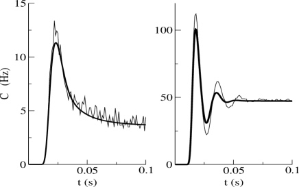
Figure 1: ACF of a LIF neuron in the sub (left) and suprathreshold regimes (right). The figures show the typical shape in both regimes: no oscillations and a large peak in the subthreshold regime ($\mu\tau_{m}<\Theta$) and damped oscillations in the suprathreshold regime ($\mu\tau_{m}>\Theta$). Thick lines are the analytical results obtained from eq.(12) (the sum has been cut at $n=200$ with $t=200ms$) and thin lines correspond to the numerical simulations of the same LIF neuron. Parameters for the subthreshold (suprathreshold)neuron are $\mu=85Hz(115Hz)$ $\sigma^{2}=6Hz(3Hz)$. Other parameters are $H=0$, $\Theta=1$, $\tau_{m}=10ms$ and $\tau_{s}=20ms$.

The analytical solution. We expand both $P(x,z,t|\hat{H},z_{0})$ and $J(z,t|z_{0})$ in powers of $\epsilon^{2}$, as $P=P_{0}+\epsilon^{2}P_{1}+0(\epsilon^{4})$ and $J=J_{0}+\epsilon^{2}J_{1}+0(\epsilon^{4})$, following a technique introduced in Mor+04 for the stationary FPE. In this expansion, the parameter $\gamma$ in eqs (5,6) is assumed to be fixed. Only at the end, when the leading orders of the expansion have been found, $\gamma$ is given its true value $\gamma=\sqrt{\tau_{m}/\tau_{s}}$.

The solution at zero-th order of the FPE (5) satisfying conditions (6,8) is

$$P_{0}(x,z,t|\hat{H},z_{0})=P(z,t|z_{0})\delta(x-X(z,t))\;,$$ (9)

where $X(z,t)$ is the time evolution of the variable $x$ obtained from eq. (3) with frozen $z$ and initial condition $\hat{H}$. Notice that $x=X(z,t)$ is a periodic function of $t$, because whenever $x=\hat{\Theta}$, $x$ is reset to $\hat{H}$. Its period, $T(z)=\tau_{m}ln(\hat{H}-\gamma z/\hat{\Theta}-\gamma z)$ ($T(z)=\infty$ for $z<\hat{\Theta}/\gamma$), is the inter-spike-interval (ISI) of a LIF neuron receiving a frozen $z$, and it is calculated from eq. (3) as the first time $T$ at which $X(z,T)=\hat{\Theta}$. After expressing the delta functions in terms of $t$, the probability density current, eq. (6), at zero-th order becomes

$$J_{0}(z,t|z_{0})=P(z,t|z_{0})\sum_{n=1}^{\infty}\delta(t-nT(z))\;.$$ (10)

This expression has a simple interpretation. The sum of delta functions in the index $n$ represents a regular train of spikes with ISI $T(z)$, as if $z$ were fixed. Therefore, the probability of having a spike along with a fluctuation $z$ at time $t$, $J_{0}$, is given at a first approximation by the product of both the probability of finding at time $t$ a spike of the train generated with frozen fluctuation $z$, and the probability of having such a fluctuation $z$ at time $t$ starting from the initial condition $z=z_{0}$, $P(z,t|z_{0})$. Note that in eq.(10) the noise is allowed to evolve in time following the distribution $P(z,t|z_{0})$. It has been proved that the stationary (frozen) distribution of $z$ can be employed to describe the firing rate of LIF neurons Mor+04 ; Mor+05 , and used the approximation that $z$ is constant during the ISIs to describe the Fano factor of non-LIF neurons with weak noise Mid+03 . However, freezing completely the noise $z$ in eq.(10) leads to very poor predictions in our problem (not shown).

To determine the ACF, eq. (7), at zero-th order, we have to the zero-th order $J(z)$ is required, which is Mor+04

$$J_{0}(z)=\nu_{0}(z)p(z)\;,$$ (11)

where $\nu_{0}(z)=1/T(z)$ for $z\geq\hat{\Theta}/\gamma$ and $\nu_{0}(z)=0$ otherwise. Finally, the zero-th order ACF is computed, after using eqs. (7,10,11) and evaluating the delta functions, as

$$C_{0}(t)=\sum_{n=1}^{\infty}\int\frac{dz_{0}\;J_{0}(z_{0})\;(\gamma z_{n}-\hat{H})(\gamma z_{n}-\hat{\Theta})}{\nu_{0}\tau_{m}n\;\gamma\;(\hat{\Theta}-\hat{H})}P(z_{n},t|z_{0})\;,$$ (12)

where $z_{n}\equiv z_{n}(t)\equiv\gamma^{-1}(\hat{\Theta}-\hat{H}e^{-t/n\tau_{m}})/(1-e^{-t/n\tau_{m}})$. The $z_{n}$s are the roots of the equations $t=nT(z_{n})$, the zeros of the delta functions in eq. (10).

In Fig. (1) we plot the ACF for the output spike train of a LIF neuron computed using eq.(12) and compare it with simulation results. The agreement is very good in both the subthreshold (left) and suprathreshold (right) regimes. In both regimes, the ACF shows a prominent peak after a relative refractory period of about $10ms$ ($\sim\tau_{m}$). This means that the potential has to be integrated from reset to threshold to emit the first spike. The prominent peak indicates that the neuron is bursty, producing spikes that are grouped within short time intervals of $20ms$ ($\sim\tau_{s}$) Mor+04 . After the prominent peak, the ACF decays to a steady-state value either monotonically (left) or with a damped oscillation (right). Damped oscillations are a robust feature in the suprathreshold regime, as is their absence in the subthreshold regime. This reflects the fact that the neuron in the suprathreshold regime fires more regularly, and therefore the output spikes tend to occur at integer number of times the mean ISI (see the peaks of the oscillations in the ACF). For long times ($t\gg\tau_{s}$) the memory of the spike at time $t=0$ has disappeared, and the ACF decays to the unconditioned probability of having a spike, that is, the firing rate of the LIF neuron.

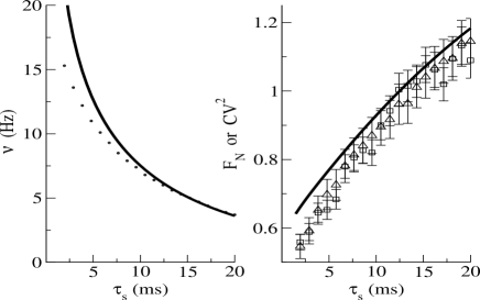
Figure 2: The firing rate (left), the Fano factor (right), $F_{N}$, and the $CV^{2}$ (right) for the output spike train of a LIF neuron are plotted as a function of $\tau_{s}$. The firing rate prediction (line) is calculated using both eqs. (13) and $\nu_{0}=\int dzJ_{0}(z)$, and it is compared with simulation results (points). The $F_{N}$ predicted by eqs. (14,12,13) (line) is compared with the $F_{N}$ (squares) and $CV^{2}$ (triangles) obtained from simulations. Parameters values are as in the subthreshold regime of Fig. (1).

The firing rate, Fano factor and CV. As it is clear, the firing rate can be obtained from the ACF, eq. (12), in the limit of long times ($t\gg\tau_{s}$). This rate has the expression

$$\nu_{0}=\lim_{t\rightarrow\infty}\sum_{n=1}^{\infty}\frac{(\gamma z_{n}(t)-\hat{H})(\gamma z_{n}(t)-\hat{\Theta})}{\sqrt{2\pi}\tau_{m}\;n\;\gamma(\hat{\Theta}-\hat{H})}\;e^{-z_{n}(t)^{2}/2}\;.$$ (13)

A different expression for the firing rate can be computed using $\nu_{0}=\int dzJ_{0}(z)$ Mor+04 . In fact, both expressions give identical results when they are plotted as a function of $\tau_{s}$ (continuous curve in Fig. (2), left). However, computationally, eq. (13) is much faster because it only involves a sum that can be cut at $n\sim 200$ (using $t=200ms$). Naturally, the number of terms needed to approximate the ACF and the firing rate grows as $t$ increases. Comparison of both expressions of $\nu_{0}$ with simulation results shows that the prediction is very good even when $\tau_{s}\sim\tau_{m}$.

The Fano factor of the output spike train, $F_{N}$, defined as the ratio between the variance of the spike count and its mean evaluated for long time windows, is directly related to the time integral of ACF as (Cox (1962) and see, e.g., eq. (3) of ref Mor+02 )

$$F_{N}=1+2\int_{0}^{\infty}dt\;(C(t)-\nu)\;.$$ (14)

We have evaluated the zero-th order $F_{N}$ in eq. (14) using the zero-th order solutions of $C(t)$ and $\nu$, eqs.(12,13). The prediction fits very well the simulation results (right panel of Fig. (2)). We have also computed the coefficient of variation of the ISIs, $CV$, of the neuron response using simulations (same panel). It is known that for renewal processes $F_{N}\equiv CV^{2}$ (e.g. for a Poisson process $F_{N}\equiv CV^{2}=1$, and $C(t)=\nu$). Here we find that $F_{N}\sim CV^{2}$ even when the output response is not a renewal process. This is because, although the synaptic time scale introduces correlations in the successive ISIs, since for low (but typical) rates $\tau_{s}<\nu^{-1}$, the correlation between successive ISIs is small. This explains the similarity between $F_{N}$ and $CV^{2}$. Notice that the firing variability is large when $\tau_{s}\geq\tau_{m}$ Mor+05 ; Svi-Des .

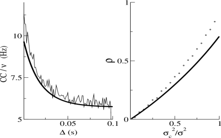
Figure 3: Left: Theoretical (thick line, eq.(17)) and simulated (thin line) CCFs normalized by the firing rate of one of the neurons as a function of time lag. Here $\sigma_{c}^{2}=2Hz$. Right: Theoretical (line, eq. (18)) and simulated (points) correlation coefficient, $\rho$, for the output spike trains of a pair of identical LIF neurons as a function of the fraction of common noise, $\sigma_{c}^{2}/\sigma^{2}$. The numerical $\rho$ is calculated using eq. (18) integrating the simulated CCF. Parameters for both figures are $\mu=85Hz$, $\sigma^{2}=9Hz$, and the others as in Fig. (1).

The crosscorrelation function and correlation coefficient. A central issue to describe population dynamics is to understand the way neuron activity synchronizes. Here we study a pair of identical LIF neurons $(k=1,2)$

$$\tau_{m}\;\dot{V_{k}}=-V_{k}+\tau_{m}\;(\;I_{k}(t)\;+\;I_{c}(t)\;)\;,$$ (15)

receiving both an independent source of current, $I_{k}(t)$, and a common source, $I_{c}(t)$. Each current is described by an equation identical to eq. (2), with mean $\mu_{ind}$ and variance $\sigma^{2}_{ind}$ for the independent components, and mean $\mu_{c}$ and variance $\sigma^{2}_{c}$ for the common component. Each neuron receives a total mean current $\mu=\mu_{ind}+\mu_{c}$ and total variance $\sigma^{2}=\sigma^{2}_{ind}+\sigma^{2}_{c}$.

The CCF of the output spike trains of the two neurons (denoted as $CC(\Delta)$) can be obtained by an analysis similar to that used for the ACF. The CCF is defined as the joint probability density of having a spike of neuron $1$ at a given time and a spike from neuron $2$ after a delay $\Delta$. Here we only summarize the main results. First, we define the normalized fluctuations $u_{k}=(I_{k}+I_{c}-\mu)/\sigma$, having zero mean and unit variance. Notice that these are not independent because of the common input $I_{c}$. Second, if neuron $1$ has a fluctuation $u_{1}$, the probability density that after a delay $\Delta$ neuron $2$ has a fluctuation $u_{2}$, $P(u_{2},\Delta|u_{1})$, is a Gaussian distribution with mean $\left<u_{2}(\Delta,u_{1})\right>=u_{1}e^{-\Delta/\tau_{s}}\sigma_{c}^{2}/\sigma^{2}$ and variance $Var(u_{2}(\Delta))=1-e^{-2\Delta/\tau_{s}}\sigma^{2}_{c}/\sigma^{2}$. Then, for long $\tau_{s}$

$$CC_{0}(\Delta)=\lim_{t\rightarrow\infty}\int du_{1}du_{2}\;P(u_{2},\Delta|u_{1})\;p(u_{1})$$

$$\;\;\;\;\;\;\ \sum_{n,m=1}^{\infty}\delta(t-nT(u_{1}))\;\delta(t+\Delta-mT(u_{2}))\;,$$ (16)

where $T(u_{k})=\tau_{m}ln(\hat{H}-\gamma u_{k}/\hat{\Theta}-\gamma u_{k})$ ($T(u_{k})=\infty$ for $u_{k}<\hat{\Theta}/\gamma$) is the ISI of the neuron $i$ receiving a constant fluctuation $u_{k}$, and $p(u_{1})$ is a normal distribution describing the steady state distribution of the fluctuations of neuron $1$. The quantities $\gamma$, $\hat{H}$ and $\hat{\Theta}$ are defined as before. The two sums of delta functions in eq. (16) can be interpreted as the product of two output spike trains with fixed ISI (determined by the input fluctuations), quantity which has to be averaged over all the possible fluctuations. The result of such an average is the CCF when the limit $t\rightarrow\infty$ is taken to allow randomization of the initial conditions, eq.(16). This equation can be simplified by integration of the delta functions, obtaining

$$CC_{0}(\Delta)=\lim_{t\rightarrow\infty}\sum_{n,m=1}^{\infty}\frac{(\gamma a_{n}-\hat{H})(\gamma b_{n}-\hat{H})}{n\;m\;\tau_{m}^{2}\;\gamma^{2}\;(\hat{\Theta}-\hat{H})^{2}}$$

$$\;\;\;\;\;(\gamma a_{m}-\hat{\Theta})(\gamma b_{m}-\hat{\Theta})P(b_{m},\Delta|a_{n})\;p(a_{n})\;,$$ (17)

where $a_{n}\equiv z_{n}(t)$ and $b_{m}\equiv z_{m}(t+\Delta)$, with $z_{n}(t)$ as in eq. (12). The theoretical CCF matches very well the simulated one (Fig. (3), left). Typically, the prediction underestimates the central peak occurring at time lag zero. The central peak of the CCF decays within a time of the order of $\tau_{s}$ (notice that the CCF is symmetric around $\Delta=0$). This is because the synaptic input, being slower than the neuron dynamics, sets its own time scale in the dynamics of interactions of the two neurons. The existence of a single peak is robust for low values of $\sigma_{c}^{2}$ in both the sub and suprathreshold regimes, but other side secondary peaks arise when all the noise is essentially common. For long $\Delta$, the CCF converges to the product of the firing rates at zero-th order, $\nu_{0}^{2}$ (see eq. (13)), because the neurons fire independently.

The correlation coefficient, $\rho$, of the spike counts for long time windows of the output spike trains of two identical neurons can be computed from their CCF (Cox (1962) and see, e.g., eq. (4) of ref Mor+02 )

$$\rho=\frac{2}{F_{N}\nu}\int_{0}^{\infty}ds\;(CC(s)-\nu^{2})\;.$$ (18)

For the two neurons in eq. (15) it can be computed at zero-th order using the zero-th orders of $CC(\Delta)$, eq.(17), $F_{N}$ and $\nu$. We have compared the theoretical and simulated $\rho$ as the fraction of common noise increases (Fig. (3), right). The prediction is good for low values of common noise, and departs from the simulations for larger values. As the common noise increases, $\rho$ increases monotonically and reaches $\rho=1$ when the common noise equals the total input noise. Correlation coefficients of $\sim 0.1$ as those found in cortex Sha+98otros are predicted accurately, and they are obtained when the common noise represents $\sim 20$ per cent of the total synaptic noise entering into the neuron, which can be a realistic value Sha+98otros . Therefore, the right plot at Fig.3 provides a valuable tool to estimate the fraction of common noise from the correlations of the spike trains of pairs of neurons, a quantity which otherwise is not available experimentally.

The results we have obtained at the cell level open the way for a systematic investigation of the role of correlations in neuronal networks.

R.M. thanks N. Rubin and J. Rinzel for their hospitality at the CNS. We thank A. Renart for his comments. R.M. and N.P. are supported by the Swartz Foundation and N.P. also by the Spanish grant BMF 2003-06242.

References

- (1) R. Moreno-Bote and N. Parga. Phys. Rev. Lett., 92(2), 028102, 2004.
- (2) M. N. Shadlen and W. T. Newsome. J. Neurosci., 18, 3870, 1998. E. Zohary and M. N. Shadlen. Nature, 370, 140, 1994.
- (3) W. Singer. Neuron, 24, 49, 1999. E. Salinas and T. J. Sejnowski. Nature Reviews Neuroscience, 2, 539, 2001. R. C. deCharms and M. M. Merzenich. Nature, 381, 610, 1996.
- (4) W. Softky and C. Koch. J. Neurosci., 13, 334, 1993.
- (5) E. Salinas and T. J. Sejnowski. J. Neurosci., 20, 6193, 2000.
- (6) R. Moreno, J. de la Rocha, A. Renart, and N. Parga. Phys. Rev. Lett., 89(2), 288101, 2002.
- (7) R. Moreno-Bote and N. Parga. Phys. Rev. Lett., 94, 088103, 2005.
- (8) G. Svirskis and J. Rinzel. Biophysical Journal, 79:629–37, 2000. A. Destexhe, M. Rudolph and D. Paré. Nat Rev Neurosci., 4(9):739, 2003.
- Ricciardi (1977) L. M. Ricciardi. Diffusion processes and related topics in biology. Springer-Verlag, Berlin, 1977.
- (10) J.W. Middleton, M.J. Chacron, B. Lindner and A. Longtin. Phys. Rev. E, 68, 021920, 2003.
- Cox (1962) D.R. Cox. Renewal theory. John-Wiley, New York,1962.