Scattering of single spikes

Abstract:

We apply the dressing method to a string solution given by a static string wrapped around the equator of a three-sphere and find that the result is the single spike solution recently discussed in the literature. Further application of the method allows the construction of solutions with multiple spikes. In particular we construct the solution describing the scattering of two single spikes and compute the scattering phase shift. As a function of the dressing parameters, the result is exactly the same as the one for the giant magnon, up to non-logarithmic terms. This suggests that the single spikes should be described by an integrable spin chain closely related to the one associated to the giant magnons. The field theory interpretation of such spin chain however is still unclear.

1 Introduction

The large-$N$ approximation [1] seems to be the most promising approach to gain an analytical understanding of the strong coupling regime of gauge theories. This belief is due in great part to the AdS/CFT correspondence [2], which provides a concrete example where such an approximation works. The correspondence argues that at large ’t Hooft coupling $\lambda$, four dimensional $SU(N)$ ${\cal N}=4$ SYM theory is described by classical strings in $AdS_{5}\times{S}^{5}$. Quantum effects on the world-sheet are suppressed by $\frac{1}{\sqrt{\lambda}}$ and string loop effects by $\frac{1}{N}$. String states can be seen to appear from the field theory [3, 4] as long gauge invariant operators. Since at large $\lambda$ a semi-classical expansion is appropriate, a particularly important role is played by classical string solutions [5, 6]. In certain limits these can be directly mapped [7, 8, 9] to spin chains which appear also in the field theory [10] as a way to describe a certain class of long operators.

For our purpose, some particular solutions recently proposed in [11, 12] and called “single spike solutions” will be of interest. They were found based on previous work [13, 14, 15] and shown to be closely related in their properties to the giant magnon solutions described in [15] and further analyzed in [16]–[38].

A very useful tool for understanding the giant magnon solutions is the dressing method of [41, 42, 43] which was shown in [44, 45] to provide a simple description of the magnon as well as a method for constructing multiple magnon solutions. Superposing magnons is in principle difficult since the problem is non-linear, and becomes possible only due to the integrability of the equations of motion. It appears natural to ask if the dressing method can be similarly applied to the study of spike solutions and their scattering.

In this paper we find that, indeed, the dressing method provides for a simple understanding of the single spike solutions and furthermore allows the construction of new solutions with multiple spikes. Of particular interest are solutions describing the scattering of two single spikes from which we can compute the scattering phase shift. This calculation is vital to gain understanding of the dynamics of two solitons in integrable systems such as this one. We find that the phase shift agrees with the one computed for the giant magnon [46] (up to non-logarithmic terms). This is perhaps surprising since both the time delay and the energy for the single spike and the giant magnon are different. Only after integrating the time delay with respect to the energy do both results agree as a function of the dressing parameters.

Another interesting conceptual advantage of the dressing method is that the “basic” or “naked” solution we need to dress to obtain the single spike is a string wrapped around the equator of the sphere infinitely many times. This confirms the idea of [11] that these solutions can be thought of as excitations over that state. Identifying this state in the field theory has however proved difficult. Some ideas in that respect including a possible relation to the antiferromagnetic state of a spin chain are discussed in [47, 48] and mentioned in [11]. However, in our mind the situation is not completely clear. It is quite interesting though, since we see that the solutions we consider have a very rich integrable dynamics.

This paper is organized as follows: in section 2 we review the main ingredients of the dressing method in the $SU(2)$ case relevant for our purposes. In sections 3 and 4 we discuss the scattering solutions for strings moving on two and three-spheres respectively. In section 5 we compute the phase shift and compare to the case of the giant magnon. Finally, we give our conclusions in section 6.

2 The dressing method

In this section we describe the basic idea of the dressing method with the main intention of establishing the notation (which is the same as in [44]) for the rest of the paper. Parameterizing $S^{3}$ with two complex coordinates $Z_{1,2}$ such that $|Z_{1}|^{2}+|Z_{2}|^{2}=1$, the Polyakov action for a string moving on ${\mathbb{R}}_{t}\times S^{3}$ is

$$S=\frac{1}{2}\int d\sigma d\tau\left[-(\partial_{\tau}t)^{2}+(\partial_{\sigma}t)^{2}+\partial_{\tau}\bar{Z}_{a}\partial_{\tau}Z_{a}-\partial_{\sigma}\bar{Z}_{a}\partial_{\sigma}Z_{a}-\Lambda\left(\bar{Z}_{a}Z_{a}-1\right)\right],$$ (2.1)

where $a=1,2$. The variable $\Lambda$ is a Lagrange multiplier which enforces $|Z_{1}|^{2}+|Z_{2}|^{2}=1$. This is supplemented by the conformal constraints, which, if we use the ansatz $t=\tau$ read

$$\partial_{\tau}\bar{Z}_{a}\partial_{\tau}Z_{a}+\partial_{\sigma}\bar{Z}_{a}\partial_{\sigma}Z_{a} = 1,$$ (2.2)

$$\partial_{\tau}\bar{Z}_{a}\partial_{\sigma}Z_{a}+\partial_{\sigma}\bar{Z}_{a}\partial_{\tau}Z_{a} = 0.$$ (2.3)

It turns out that if we define the $SU(2)$ matrix

$$g=\left(\begin{array}[]{cc}Z_{1}&-iZ_{2}\\ -i\bar{Z}_{2}&\bar{Z}_{1}\end{array}\right),$$ (2.4)

then the equations of motion and the constraints can be written together in a compact form as

$$\bar{\partial}\left(\partial gg^{-1}\right)+\partial\left(\bar{\partial}gg^{-1}\right)=0,$$ (2.5)

where we defined $z=\frac{1}{2}(\sigma-\tau)$, $\bar{z}=\frac{1}{2}(\sigma+\tau)$ and $\partial=\partial_{z}$, $\bar{\partial}=\partial_{\bar{z}}$. Eq. (2.5) can be seen as the compatibility equation for the existence of a solution to the linear problem

$$i\bar{\partial}\Psi=\frac{A\Psi}{1+\lambda},\ \ \ \ \ i\partial\Psi=\frac{B\Psi}{1-\lambda},$$ (2.6)

where

$$A=i\bar{\partial}gg^{-1},\ \ \ \ \ B=i\partial gg^{-1},$$ (2.7)

and $\Psi$ is a two by two matrix. Given $g$ satisfying eq.(2.5) we can find $\Psi$ satisfying eq.(2.6) with the initial condition $\Psi(\lambda=0)=g$. Conversely, if we have a solution $\Psi(\lambda,z,\bar{z})$ for given matrices $A(z,\bar{z})$ and $B(z,\bar{z})$ then $\Psi(0)$ is guaranteed to satisfy eq.(2.5). Notice that for this we need $A$ and $B$ independent of $\lambda$.

The basic point of the dressing method is that given a solution $g$, from which $A$, $B$ and $\Psi$ can be determined, one can then find a new solution by multiplying $\Psi$ by an appropriate matrix $\chi(\lambda)$: $\Psi\rightarrow\chi\Psi$. Only for specific choices of $\chi$ will the product $\chi\Psi$ continue to satisfy the desired eq.(2.6). In the examples we consider, the matrix $\chi$ takes the form

$$\chi(\lambda)=1+\frac{\lambda_{1}-\bar{\lambda}_{1}}{\lambda-\lambda_{1}}P,$$ (2.8)

where $\lambda_{1}$ an arbitrary complex parameter and $P$ is a projector defined as

$$P=\frac{\Psi(\bar{\lambda}_{1})ee^{\dagger}\Psi^{-1}(\lambda_{1})}{e^{\dagger}\Psi^{-1}(\lambda_{1})\Psi(\bar{\lambda}_{1})e},$$ (2.9)

in terms of a vector $e$ that can be set to $e=(1,1)$ without loss of generality. The rationale behind the choice (2.8) can be found in the references [44, 41, 42, 43] together with a more complete explanation of the method. For us it suffices to know that, given a solution $g(z,\bar{z})$ this method then provides a one (complex) parameter family of new solutions $g_{\lambda_{1}}(z,\bar{z})$ labeled by the complex number $\lambda_{1}$. Successive applications of the dressing method can be used to generate more complicated solutions depending on additional parameters $\lambda_{2},\lambda_{3},\ldots$. The examples in the following sections should clarify how to apply this method in practice.

3 Single spikes on $S^{2}$

In this section we consider the solutions for strings on $S^{2}$ discussed in [11, 12] and demonstrate how to generalize them to include many spikes. As a first step we rewrite the solution from [11], which lives inside an $S^{2}\subset S^{5}$, in terms of six real embedding coordinates $Y^{i}$ on $S^{5}$ as

$$Y^{1} = {1\over 2}(Z^{1}+\overline{Z}^{1})=\sqrt{1-\cos^{2}\theta_{1}\mathop{\mathrm{sech}}\nolimits^{2}\xi\over 1+\cot^{2}\theta_{1}\tanh^{2}\xi}\left[\cos x+\sin x\cot\theta_{1}\tanh\xi\right],$$ (3.10)

$$Y^{2} = {1\over 2i}(Z^{1}-\overline{Z}^{1})=\sqrt{1-\cos^{2}\theta_{1}\mathop{\mathrm{sech}}\nolimits^{2}\xi\over 1+\cot^{2}\theta_{1}\tanh^{2}\xi}\left[\sin x-\cos x\cot\theta_{1}\tanh\xi\right],$$ (3.11)

$$Y^{3} = Z^{2}=\cos\theta_{1}\mathop{\mathrm{sech}}\nolimits\xi,$$ (3.12)

$$Y^{4} = Y^{5}=Y^{6}=0,$$ (3.13)

where $\theta_{1}$ is a parameter of the solution and

$$\xi=t\sec\theta_{1}+x\tan\theta_{1}.$$ (3.14)

Let us call the solution (3.10) $\vec{Y}_{1}$.

The simplest way to build a scattering state of this spike $\vec{Y}_{1}$ with another spike $\vec{Y}_{2}$ (which is given by the same formula as above but with a different parameter $\theta_{2}$) is to use the formula [49]

$$\vec{Y}_{1,2}=\vec{Y}_{0}+(\vec{Y}_{1}-\vec{Y}_{2}){\vec{Y}_{0}\cdot\vec{Y}_{2}-\vec{Y}_{0}\cdot\vec{Y}_{1}\over 1-\vec{Y}_{1}\cdot\vec{Y}_{2}},$$ (3.15)

where $\vec{Y}_{0}$ is the “vacuum” or “naked” solution, which in this context is given by

$$Y_{0}=(\cos x,\sin x,0,0,0,0),$$ (3.16)

and describes the string at rest winding infinitely many times around the equator ($\theta_{0}=\pi/2$).

One can check directly that (3.15) satisfies the equations of motion and Virasoro constraints

$$-\partial_{t}^{2}\vec{Y}+\partial_{x}^{2}\vec{Y}+(-\partial_{t}\vec{Y}\cdot\partial_{t}\vec{Y}+\partial_{x}\vec{Y}\cdot\partial_{x}\vec{Y})\vec{Y} = 0,$$ (3.17)

$$-\partial_{t}\vec{Y}\cdot\partial_{x}\vec{Y} = 0,$$ (3.18)

$$\partial_{t}\vec{Y}\cdot\partial_{t}\vec{Y}+\partial_{x}\vec{Y}\cdot\partial_{x}\vec{Y} = 1,$$ (3.19)

and of course the embedding constraint $\vec{Y}\cdot\vec{Y}=1$. Further application of the method would allow us to construct solutions with more spikes but for our present purpose these two-spike solutions are sufficient.

It is important to note that one must first switch to the $(t,x)$ coordinates

$$\tau=t\sec\theta_{1},\qquad\sigma=x\sec\theta_{1}$$ (3.20)

before applying the relation (3.15). That is, from eq.(3.20) it is clear that the $\sigma$ and $\tau$ coordinates of the solutions $\vec{Y}_{1}$ and $\vec{Y}_{2}$ are normalized differently; they cannot be combined using eq.(3.15) until we first switch to the common $(t,x)$ coordinates. We now turn to the case of single spikes on $S^{3}$ where the solution has an additional angular momentum parameter.

4 Single spikes on $S^{3}$ and scattering solutions via dressing

As noted in the previous section, to superpose spikes it is important to rescale $\sigma$ and $\tau$ so that the relation $t=\kappa\tau$ holds with $\kappa=1$ for all solutions. Going to conformal gauge and using the same ideas as in the previous case we find a solution depending on two parameters $\theta_{1}$ and $\gamma_{1}$. If we now use the parameterization

$$Z_{1} = Y_{1}+iY_{2}=\sin\theta e^{i\phi_{1}},$$ (4.21)

$$Z_{2} = Y_{3}+iY_{4}=\cos\theta e^{i\phi_{2}},$$ (4.22)

$$Z_{3} = Y_{5}+iY_{6}=0,$$ (4.23)

of $S^{3}$ in terms of three angles $(\theta,\phi_{1},\phi_{2})$, the solution is

$$\cos\theta = \frac{\cos\theta_{1}}{\cosh\xi},$$ (4.24)

$$\phi_{1} = \sigma-\arctan\left(\frac{\cos\theta_{1}}{\sin\theta_{1}}\tanh\xi\right),$$ (4.25)

$$\phi_{2} = \frac{\sin\gamma_{1}}{1-\cos^{2}\gamma_{1}\sin^{2}\theta_{1}}\left(\sigma+\tau\,\cos\gamma_{1}\sin\theta_{1}\right),$$ (4.26)

$$\xi = \frac{\cos\theta_{1}\cos\gamma_{1}}{1-\cos^{2}\gamma_{1}\sin^{2}\theta_{1}}\left(\tau+\sigma\,\cos\gamma_{1}\sin\theta_{1}\right).$$ (4.27)

This solution has one more conserved angular momentum and lives in an $S^{3}\subset S^{5}$. Its properties were studied in [11]. Now we show that this solution follows from the infinitely wrapped string by using the same dressing method that in [44] was used for giant magnons.

From now on we set $Z_{3}=0$ and consider, as mentioned, solutions on ${\mathbb{R}}_{t}\times S^{3}$ where the $S^{3}$ is parameterized by $Z_{1,2}$ with $|Z_{1}|^{2}+|Z_{2}|^{2}=1$. This allows us to apply the ideas described in section 2 directly. We start from the infinitely wrapped string solution

$$Z_{1}=e^{i\sigma},\ \ \ Z_{2}=0.$$ (4.28)

The embedding into $SU(2)$ with $z=\frac{1}{2}(\sigma-t)$ and $\bar{z}=\frac{1}{2}(\sigma+t)$ is given by

$$g=\left(\begin{array}[]{cc}e^{i(z+\bar{z})}&0\\ 0&e^{-i(z+\bar{z})}\end{array}\right),$$ (4.29)

which leads to (using the notation from [44] or section 2)

$$A=B=\left(\begin{array}[]{cc}-1&0\\ 0&1\end{array}\right).$$ (4.30)

The solution of the corresponding linear problem (2.6) is

$$\Psi=\left(\begin{array}[]{cc}e^{iZ(\lambda)}&0\\ 0&e^{-iZ(\lambda)}\end{array}\right),\ \ \ Z(\lambda)=\frac{z}{1-\lambda}+\frac{\bar{z}}{1+\lambda}.$$ (4.31)

Taking the constant vector $e=(1,1)$ we obtain the projection operator

$$P=\frac{1}{1+e^{2i(Z(\lambda_{1})-Z(\bar{\lambda}_{1}))}}\left(\begin{array}[]{cc}1&e^{2iZ(\lambda_{1})}\\ e^{-2iZ(\bar{\lambda}_{1})}&e^{2i(Z(\lambda_{1})-Z(\bar{\lambda}_{1}))}\end{array}\right).$$ (4.32)

The method then gives a family of new solutions (after including a normalization factor to maintain $\det\Psi(\lambda=0)=1$)

$$g_{\lambda_{1}}=\Psi_{\lambda_{1}}(0)=\sqrt{\frac{\lambda_{1}}{\bar{\lambda}_{1}}}\left[1-\frac{\lambda_{1}-\bar{\lambda}_{1}}{\lambda_{1}}P\right]\Psi(\lambda=0).$$ (4.33)

We can now read off the coordinates $Z_{1,2}$ of this solution, finding

$$Z_{1} = \frac{e^{i\sigma}}{\sqrt{\lambda_{1}\bar{\lambda}_{1}}}\frac{\lambda_{1}e^{-2iZ(\bar{\lambda}_{1})}+\bar{\lambda}_{1}e^{-2iZ(\lambda_{1})}}{e^{-2iZ(\lambda_{1})}+e^{-2iZ(\bar{\lambda}_{1})}},$$ (4.34)

$$Z_{2} = \frac{e^{-i\sigma}}{\sqrt{\lambda_{1}\bar{\lambda}_{1}}}\frac{i(\bar{\lambda}_{1}-\lambda_{1})}{e^{-2iZ(\lambda_{1})}+e^{-2iZ(\bar{\lambda}_{1})}}.$$ (4.35)

The energy and angular momentum can be computed as

$$\varepsilon=E-T\Delta\phi = \frac{\sqrt{\lambda}}{2\pi}\int_{-\infty}^{+\infty}d\sigma\left(1-\partial_{\sigma}{\rm Im}\left[\log Z_{1}\right]\right),$$ (4.36)

$$J_{i} = \frac{\sqrt{\lambda}}{2\pi}\int_{-\infty}^{+\infty}d\sigma\,{\rm Im}\left[\bar{Z}_{i}\partial_{t}Z_{i}\right],\quad i=1,2$$ (4.37)

where $\lambda$ is the ’t Hooft coupling. The energy itself $E=\frac{\sqrt{\lambda}}{2\pi}\int_{-\infty}^{\infty}d\sigma$ is infinite but the excitation energy $\varepsilon$ above the infinitely wrapped string “vacuum” is finite. Henceforth we will usually refer to $\varepsilon$ as the energy of the solution.

Substituting (4.34) into (4.36) and choosing to parameterize $\lambda_{1}$ via

$$\lambda_{1}=re^{ip/2},$$ (4.38)

where $0<r<\infty$, $-\pi<\frac{p}{2}<\pi$, we obtain

$$\varepsilon=\frac{\sqrt{\lambda}}{\pi}\left[\frac{\pi}{2}-\left|\left|\frac{p}{2}\right|-\frac{\pi}{2}\right|\right]=\left\{\begin{array}[]{ll}\frac{\sqrt{\lambda}}{\pi}\left|\frac{p}{2}\right|,&\quad\textrm{if}\ \left|\frac{p}{2}\right|<\frac{\pi}{2}\\ &\\ \frac{\sqrt{\lambda}}{\pi}\left(\pi-\left|\frac{p}{2}\right|\right),&\quad\textrm{if}\ \left|\frac{p}{2}\right|>\frac{\pi}{2}\\ \end{array}\right.$$ (4.39)

which is plotted in fig.1 for convenience. Notice that the energy is always positive.

Figure 1: Excitation energy of the single spike solution as a function of the parameter $\frac{p}{2}$.

Similarly, equations (4.37), (4.34), and (4.35) lead to

$$J_{1} = \mathrm{sign}\left(\sin p\right)\,\frac{\sqrt{\lambda}}{i4\pi}\left[\left(\lambda_{1}-\frac{1}{\lambda_{1}}\right)-\left(\bar{\lambda}_{1}-\frac{1}{\bar{\lambda}_{1}}\right)\right]$$ (4.40)

$$= \mathrm{sign}\left(\sin p\right)\,\frac{\sqrt{\lambda}}{\pi}\frac{1+r^{2}}{2r}\sin\frac{p}{2},$$

$$J_{2} = \mathrm{sign}\left(\sin p\right)\,\frac{\sqrt{\lambda}}{i4\pi}\left[\left(\lambda_{1}+\frac{1}{\lambda_{1}}\right)-\left(\bar{\lambda}_{1}+\frac{1}{\bar{\lambda}_{1}}\right)\right]$$ (4.41)

$$= \mathrm{sign}\left(\sin p\right)\,\frac{\sqrt{\lambda}}{\pi}\frac{r^{2}-1}{2r}\sin\frac{p}{2}.$$

Upon eliminating $r$ in the above equations we find that the two angular momenta are related by

$$J_{1}=\sqrt{J_{2}^{2}+\frac{\lambda}{\pi^{2}}\sin^{2}\frac{p}{2}},$$ (4.42)

One can check that equations (4.39) and (4.42) agree with the expressions obtained in [11] for the single spike solution when we identify the parameter $\bar{\theta}$ there with $p/2=\bar{\theta}$. In [11] only the case $0<\bar{\theta}<\frac{\pi}{2}$ was considered, whereas here we can take $-\pi<\bar{\theta}<\pi$. Extending the range of $\bar{\theta}$ includes solutions which are related by reflections to the solutions in the $0<\bar{\theta}<\frac{\pi}{2}$ range and therefore are not truly independent (they are just spikes moving in the opposite direction). Shortly we will superpose solutions and it will be important to consider single spikes in the full range $-\pi<\bar{\theta}<\pi$.

As a reminder, in terms of the same dressing parameter $\lambda_{1}=re^{i\frac{p}{2}}$, for the giant magnon solution of [15], the energy and angular momentum are given by (see [44]),

$$E^{(\rm{mag})} = \frac{\sqrt{\lambda}}{i4\pi}\mathrm{sign}(\sin\frac{p}{2})\left[\left(\lambda_{1}-\frac{1}{\lambda_{1}}\right)-\left(\bar{\lambda}_{1}-\frac{1}{\bar{\lambda}_{1}}\right)\right]=\frac{\sqrt{\lambda}}{\pi}\frac{1+r^{2}}{2r}\left|\sin\frac{p}{2}\right|,$$ (4.43)

$$J_{2}^{(\rm{mag})} = -\frac{\sqrt{\lambda}}{i4\pi}\mathrm{sign}(\sin\frac{p}{2})\left[\left(\lambda_{1}+\frac{1}{\lambda_{1}}\right)-\left(\bar{\lambda}_{1}+\frac{1}{\bar{\lambda}_{1}}\right)\right]=\frac{\sqrt{\lambda}}{\pi}\frac{1-r^{2}}{2r}\left|\sin\frac{p}{2}\right|.$$ (4.44)

Eliminating $r$ in these equations leads to the relation

$$E^{(\rm{mag})}=\sqrt{\{J_{2}^{(\rm{mag})}\}^{2}+\frac{\lambda}{\pi^{2}}\sin^{2}\frac{p}{2}}.$$ (4.45)

Going back to the spike solution and repeating the dressing method again, from a single two-charge soliton we obtain a two spike solution

$$Z_{1} = \frac{e^{i\sigma}}{2|\lambda_{1}\lambda_{2}|}\frac{R+|\lambda_{1}|^{2}\lambda_{1\bar{1}}\lambda_{2\bar{2}}e^{+i(v_{1}-v_{2})}+|\lambda_{2}|^{2}\lambda_{1\bar{1}}\lambda_{2\bar{2}}e^{-i(v_{1}-v_{2})}}{\lambda_{12}\lambda_{\bar{1}\bar{2}}\cosh(u_{1}+u_{2})+\lambda_{1\bar{2}}\lambda_{\bar{1}2}\cosh(u_{1}-u_{2})+\lambda_{1\bar{1}}\lambda_{2\bar{2}}\cos(v_{1}-v_{2})},$$

$$Z_{2} = \frac{-i}{2|\lambda_{1}\lambda_{2}|}\frac{\lambda_{1\bar{1}}e^{iv_{1}}\left[\lambda_{12}\lambda_{\bar{1}2}\bar{\lambda}_{2}e^{+u_{2}}+\lambda_{\bar{1}\bar{2}}\lambda_{1\bar{2}}\lambda_{2}e^{-u_{2}}\right]+(1\leftrightarrow 2)}{\lambda_{12}\lambda_{\bar{1}\bar{2}}\cosh(u_{1}+u_{2})+\lambda_{1\bar{2}}\lambda_{\bar{1}2}\cosh(u_{1}-u_{2})+\lambda_{1\bar{1}}\lambda_{2\bar{2}}\cos(v_{1}-v_{2})},$$

where

$$R=\lambda_{12}\lambda_{\bar{1}\bar{2}}\left[\lambda_{1}\lambda_{2}e^{+u_{1}+u_{2}}+\bar{\lambda}_{1}\bar{\lambda}_{2}e^{-u_{1}-u_{2}}\right]+\lambda_{\bar{1}2}\lambda_{1\bar{2}}\left[\lambda_{1}\bar{\lambda}_{2}e^{+u_{1}-u_{2}}+\bar{\lambda}_{1}\lambda_{2}e^{-u_{1}+u_{2}}\right],$$ (4.48)

and

$$u_{i} = i(Z(\lambda_{i})-Z(\bar{\lambda}_{i})),$$

$$v_{i} = Z(\lambda_{i})+Z(\bar{\lambda}_{i})-\sigma,\quad i=1,2.$$ (4.49)

The following shorthand notation has been used:

$$\lambda_{12}=\lambda_{1}-\lambda_{2},\quad\lambda_{1\bar{2}}=\lambda_{1}-\bar{\lambda}_{2},\quad{\rm etc.}$$ (4.50)

Substituting $\lambda_{i}=r_{i}e^{ip_{i}/2}$, we can express $|Z_{2}|$ as a function of $t$ and $\sigma$. To gain some understanding of the solution we plot $|Z_{2}|$ as a function of $\sigma$ for different values of $t=\tau$ in fig.2. At an early time the spikes are far apart. However they come close, eventually scattering and separating from each other. At late times, the profile again describes two separated solitons, the only evidence of the scattering being that their positions are shifted with respect to what they would be if they had moved past each other with constant velocity. Numerically we can compute the shift and from there the time delay, namely the difference between the time at which the soliton arrives to a given point and the time at which it would have arrived if it had not met the other soliton in the way. This serves to illustrate the analytical calculations we perform in the next section and the numerical results also provide a useful check. As a final point, since when $t\rightarrow-\infty$ the solitons are far apart, the energy and angular momenta of the solution is simply the sum of the ones for each soliton separately.

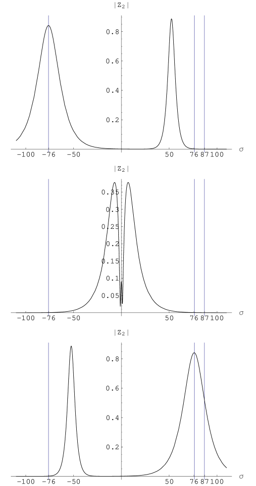
Figure 2: $|Z_{2}|$ as a function of $\sigma$ with the choice of parameters $r_{1}=0.24,\ p_{1}=2.0,\ r_{2}=0.50,$ and $p_{2}=4.1$ at $t=-20,\ 0,\ 20$, from top to bottom, respectively. The line at $\sigma=87$ is the expected final location of the first soliton had it not encountered the second soliton. The velocity and distance shift of the first soliton are, $V_{1}=4.08$ and $\delta\sigma_{1}=10.7$, respectively, which agree with the analytic result given in the text.

5 Scattering phase shift

To compute the time delay, we first consider a single soliton as given by eq.(4.35). Using this together with eq.(4.49), we obtain,

$$\left|Z_{2}\right|\propto\frac{1}{\cosh u_{1}}.$$ (5.51)

This shows that the position of the soliton, namely, the maximum of $|Z_{2}|$, is determined by equating $u_{1}=0$. In particular this implies that the soliton moves with constant velocity

$$V_{i}=\frac{1+\lambda_{i}\bar{\lambda}_{i}}{\lambda_{i}+\bar{\lambda}_{i}}=\frac{1+r_{i}^{2}}{2r_{i}\cos\frac{p_{i}}{2}},\quad i=1,2.$$ (5.52)

We can make this explicit by writing

$$u_{i}=\frac{i(\lambda_{i}^{2}-\bar{\lambda}_{i}^{2})}{\left|1-\lambda_{i}^{2}\right|^{2}}(\sigma-V_{i}t),\quad i=1,2.$$ (5.53)

Now we compute the time delay that particle 1 experiences as it goes through the other particle assuming particle 1 starts from the left. They can be moving toward each other ($V_{2}<0<V_{1}$) or in the same direction ($0<V_{2}<V_{1}$). To find the distance shift that particle 1 experiences, we first compute the location of the particle when $\sigma,t\rightarrow-\infty$. We can obtain the location by computing the extremum of eq.(LABEL:ZZ_2) with respect to $u_{1}$ and then equate the result with eq.(5.53) in this limit. The initial location of particle one at $t=-t_{0}$ is,

$$\sigma_{i}(t=-t_{0})=\sigma_{1}(\sigma,t\rightarrow-\infty)=-V_{1}t_{0}+\mathrm{sign}\left(\sin p_{2}\right)\,\frac{i\left|1-\bar{\lambda}_{1}^{2}\right|^{2}}{2(\lambda_{1}^{2}-\bar{\lambda}_{1}^{2})}\log\left[\frac{\lambda_{12}\lambda_{\bar{1}\bar{2}}}{\lambda_{1\bar{2}}\lambda_{\bar{1}2}}\right].$$ (5.54)

Similarly at the other limit, we obtain the final location of the particle at $t=+t_{0}$,

$$\sigma_{f}(t=+t_{0})=\sigma_{1}(\sigma,t\rightarrow+\infty)=V_{1}t_{0}-\mathrm{sign}\left(\sin p_{2}\right)\,\frac{i\left|1-\bar{\lambda}_{1}^{2}\right|^{2}}{2(\lambda_{1}^{2}-\bar{\lambda}_{1}^{2})}\log\left[\frac{\lambda_{12}\lambda_{\bar{1}\bar{2}}}{\lambda_{1\bar{2}}\lambda_{\bar{1}2}}\right],$$ (5.55)

whereas the expected location of particle 1 in the limit, from eq.(5.54), is

$$\sigma_{exp}=\sigma_{i}(t=-t_{0})+2V_{1}t_{0}=V_{1}t_{0}+\mathrm{sign}\left(\sin p_{2}\right)\,\frac{i\left|1-\bar{\lambda}_{1}^{2}\right|^{2}}{2(\lambda_{1}^{2}-\bar{\lambda}_{1}^{2})}\log\left[\frac{\lambda_{12}\lambda_{\bar{1}\bar{2}}}{\lambda_{1\bar{2}}\lambda_{\bar{1}2}}\right].$$ (5.56)

Thus, the distance shift that particle 1 experiences as it goes through the other particle starting from the left is

$$\delta\sigma_{1} = \sigma_{exp}-\sigma_{f}$$ (5.57)

$$= \mathrm{sign}\left(\sin p_{2}\right)\,\frac{i(1-\lambda_{1}^{2})(1-\bar{\lambda}_{1}^{2})}{(\lambda_{1}^{2}-\bar{\lambda}_{1}^{2})}\log\left[\frac{\lambda_{12}\lambda_{\bar{1}\bar{2}}}{\lambda_{1\bar{2}}\lambda_{\bar{1}2}}\right]$$ (5.58)

$$= \mathrm{sign}\left(\sin p_{2}\right)\,\frac{1+r_{1}^{4}-2r_{1}^{2}\cos p_{1}}{2r_{1}^{2}\sin p_{1}}\log\left[\frac{r_{1}^{2}+r_{2}^{2}-2r_{1}r_{2}\cos\frac{p_{1}-p_{2}}{2}}{r_{1}^{2}+r_{2}^{2}-2r_{1}r_{2}\cos\frac{p_{1}+p_{2}}{2}}\right].$$ (5.59)

Finally, the time delay for particle 1 becomes

$$\Delta T_{1} = \frac{\delta\sigma_{1}}{V_{1}}=\mathrm{sign}\left(\sin p_{2}\right)\,\frac{i(1-\lambda_{1}^{2})(1-\bar{\lambda}_{1}^{2})}{(\lambda_{1}-\bar{\lambda}_{1})(1+\lambda_{1}\bar{\lambda}_{1})}\log\left[\frac{\lambda_{12}\lambda_{\bar{1}\bar{2}}}{\lambda_{1\bar{2}}\lambda_{\bar{1}2}}\right]$$ (5.60)

$$= \mathrm{sign}\left(\sin p_{2}\right)\,\frac{1+r_{1}^{4}-2r_{1}^{2}\cos p_{1}}{2r_{1}(1+r_{1}^{2})\sin\frac{p_{1}}{2}}\log\left[\frac{r_{1}^{2}+r_{2}^{2}-2r_{1}r_{2}\cos\frac{p_{1}-p_{2}}{2}}{r_{1}^{2}+r_{2}^{2}-2r_{1}r_{2}\cos\frac{p_{1}+p_{2}}{2}}\right].$$

For comparison, the velocity, position shift and time delay for the scattering of giant magnons are

$$V_{i}^{(\rm{mag})} = \frac{\lambda_{i}+\bar{\lambda}_{i}}{1+\lambda_{i}\bar{\lambda}_{i}}=\frac{2r_{i}\cos\frac{p_{i}}{2}}{1+r_{i}^{2}},$$ (5.61)

$$\delta\sigma_{1}^{(\rm{mag})} = \mathrm{sign}(\sin\frac{p_{2}}{2})i\frac{(1-\lambda_{1}^{2})(1-\bar{\lambda}_{1}^{2})}{(\lambda_{1}-\bar{\lambda}_{1})(1+\lambda_{1}\bar{\lambda}_{1})}\log\left[\frac{\lambda_{12}\lambda_{\bar{1}\bar{2}}}{\lambda_{1\bar{2}}\lambda_{\bar{1}2}}\right]$$ (5.62)

$$= \mathrm{sign}(\sin\frac{p_{2}}{2})\frac{1+r_{1}^{4}-2r_{1}^{2}\cos p_{1}}{2r_{1}(1+r_{1}^{2})\sin\frac{p_{1}}{2}}\log\left[\frac{r_{1}^{2}+r_{2}^{2}-2r_{1}r_{2}\cos\frac{p_{1}-p_{2}}{2}}{r_{1}^{2}+r_{2}^{2}-2r_{1}r_{2}\cos\frac{p_{1}+p_{2}}{2}}\right],$$

$$\Delta T_{1}^{(\rm{mag})} = \mathrm{sign}(\sin\frac{p_{2}}{2})i\frac{(1-\lambda_{1}^{2})(1-\bar{\lambda}_{1}^{2})}{(\lambda_{1}^{2}-\bar{\lambda}_{1}^{2})}\log\left[\frac{\lambda_{12}\lambda_{\bar{1}\bar{2}}}{\lambda_{1\bar{2}}\lambda_{\bar{1}2}}\right]$$ (5.63)

$$= \mathrm{sign}(\sin\frac{p_{2}}{2})\frac{1+r_{1}^{4}-2r_{1}^{2}\cos p_{1}}{2r_{1}^{2}\sin p_{1}}\log\left[\frac{r_{1}^{2}+r_{2}^{2}-2r_{1}r_{2}\cos\frac{p_{1}-p_{2}}{2}}{r_{1}^{2}+r_{2}^{2}-2r_{1}r_{2}\cos\frac{p_{1}+p_{2}}{2}}\right].$$ (5.64)

Note that the distance shift and time delay are interchanged compared to those of the spikes.

We can now compute the phase shift with the formula

$$\left(\frac{\partial\delta_{1}}{\partial\varepsilon_{1}}\right)_{J_{2}}=\Delta T_{1},$$ (5.65)

where the angular momentum, $J_{2}$ must be fixed when the above equation is integrated. It is easy to check that the integral is given by the same function $\Theta$ that appears in the giant magnon calculation of [46]

$$\Theta\left(\lambda_{1},\bar{\lambda}_{1},\lambda_{2},\bar{\lambda}_{2}\right)=\frac{\sqrt{\lambda}}{2\pi}\left[K\left(\lambda_{1},\lambda_{2}\right)+K\left(\bar{\lambda}_{1},\bar{\lambda}_{2}\right)-K\left(\lambda_{1},\bar{\lambda}_{2}\right)-K\left(\bar{\lambda}_{1},\lambda_{2}\right)\right],$$ (5.66)

where the function $K$ is given by

$$K\left(X,Y\right)=\left[\left(X+\frac{1}{X}\right)-\left(Y+\frac{1}{Y}\right)\right]\log(X-Y).$$ (5.67)

Indeed, using eqns.(4.39), (4.40) and (4.41) we can compute

$$\left(\frac{\partial\lambda_{1}}{\partial\varepsilon_{1}}\right)_{J_{2}}=\mathrm{sign}\left(\sin p_{1}\right)\,\frac{2\pi}{\sqrt{\lambda}}\frac{i\lambda_{1}^{2}(1-\bar{\lambda}_{1}^{2})}{(\lambda_{1}-\bar{\lambda}_{1})(1+\lambda_{1}\bar{\lambda}_{1})},\ \ \ \ \ \left(\frac{\partial\bar{\lambda}_{1}}{\partial\varepsilon_{1}}\right)_{J_{2}}=\overline{\left(\frac{\partial\lambda_{1}}{\partial\varepsilon_{1}}\right)}_{J_{2}},$$ (5.68)

and then use them to differentiate $\Theta$ in eq.(5.66) with respect to $\varepsilon_{1}$. We obtain,

$$\left(\frac{\partial\Theta}{\partial\varepsilon_{1}}\right)_{J_{2}} = -\mathrm{sign}(\sin p_{1}\sin p_{2})\Delta T_{1}+\mathrm{sign}\left(\sin p_{1}\right)\,\frac{i(\lambda_{2}-\bar{\lambda}_{2})}{\lambda_{2}\bar{\lambda}_{2}}$$ (5.69)

$$= -\mathrm{sign}(\sin p_{1}\sin p_{2})\frac{\partial\delta_{1}}{\partial\varepsilon_{1}}-\mathrm{sign}(\sin p_{1}\sin p_{2})\frac{2\pi}{\sqrt{\lambda}}\left(J_{1}^{(2)}-J_{2}^{(2)}\right),$$ (5.70)

where $J_{1}^{(2)}$ and $J_{2}^{(2)}$ are the angular momenta of the second soliton.

The phase shift that particle 1 experiences as it goes through particle 2 is then,

$$\delta_{1} = -\mathrm{sign}(\sin p_{1}\sin p_{2})\Theta\left(\lambda_{1},\bar{\lambda}_{1},\lambda_{2},\bar{\lambda}_{2}\right)+\mathrm{sign}\left(\sin p_{2}\right)\,\frac{i(\lambda_{2}-\bar{\lambda}_{2})}{\lambda_{2}\bar{\lambda}_{2}}\varepsilon_{1}$$ (5.71)

$$= -\mathrm{sign}(\sin p_{1}\sin p_{2})\Theta\left(\lambda_{1},\bar{\lambda}_{1},\lambda_{2},\bar{\lambda}_{2}\right)-\frac{2\pi}{\sqrt{\lambda}}\left(J_{1}^{(2)}-J_{2}^{(2)}\right)\varepsilon_{1}.$$ (5.72)

The phase shift for the giant magnon is known from [46] to be,

$$\delta_{1}^{(\rm{mag})}=-\mathrm{sign}(\sin\frac{p_{1}}{2}\sin\frac{p_{2}}{2})\Theta\left(\lambda_{1},\bar{\lambda}_{1},\lambda_{2},\bar{\lambda}_{2}\right)-\left(\varepsilon_{2}+J_{2}^{(\rm{mag},2)}\right)p_{1}.$$ (5.73)

Remarkably we see a perfect parallel between the two results, despite the fact that intermediate steps are different. Ignoring a possible sign, the phase shift is the same up to non-logarithmic terms. The non-logarithmic terms are in any case non-universal. For the scattering of giant magnons [15] such terms were absorbed by redefining the coordinate $\sigma$ in agreement with the expectations from the spin chain side. Here we do not clearly know the spin chain description of the system so we do not have any guide about how to treat the non-logarithmic terms. We leave this point for future understanding when the dual spin chain system is better known. A clue in this respect is that the giant magnon phase appears as the strong-coupling limit of the scattering phase proposed in [51] from field theory considerations. Presumably, since the phase for scattering of single spikes is the same as for giant magnons, the AFS phase also plays a role in understanding these new solutions.

6 Conclusions

In this paper we have shown that the recently studied single spike solutions follow very simply as excitations of the string wrapped around the equator by applying the dressing method. This allows us to find more generic solutions where the profile of the string is not rigid. In particular, we found a solution describing the scattering of two spikes and calculated the corresponding phase shift. Perhaps surprisingly the result is the same as for the giant magnon when written in terms of the dressing parameters, even though intermediate steps in the calculation were quite different. This shows that the same integrable structure lies behind both and should perhaps give a clue to the spin chain description of the single spike solutions which is still missing.

Note Added

While this paper was being written, [52] appeared which has some overlap with section 4. Also, in that paper an interesting field theory interpretation of these solutions is proposed. The phase shift we compute here might be useful to test that proposal.

References

- [1] G. ’t Hooft, “A Two-Dimensional Model For Mesons,” Nucl. Phys. B 75, 461 (1974).
-
[2]
J. Maldacena,
“The large limit of superconformal field theories and supergravity,”
Adv. Theor. Math. Phys. 2, 231 (1998)
[Int. J. Theor. Phys. 38, 1113 (1998)],
hep-th/9711200,
S. S. Gubser, I. R. Klebanov and A. M. Polyakov, “Gauge theory correlators from non-critical string theory,” Phys. Lett. B 428, 105 (1998) [arXiv:hep-th/9802109],
E. Witten, “Anti-de Sitter space and holography,” Adv. Theor. Math. Phys. 2, 253 (1998) [arXiv:hep-th/9802150],
- [3] D. Berenstein, J. M. Maldacena and H. Nastase, “Strings in flat space and pp waves from N = 4 super Yang Mills,” JHEP 0204, 013 (2002) [arXiv:hep-th/0202021].
- [4] S. S. Gubser, I. R. Klebanov and A. M. Polyakov, “A semi-classical limit of the gauge/string correspondence,” Nucl. Phys. B 636, 99 (2002) [arXiv:hep-th/0204051].
- [5] S. Frolov and A. A. Tseytlin, “Multi-spin string solutions in ,” Nucl. Phys. B 668, 77 (2003) [arXiv:hep-th/0304255]. “Rotating string solutions: AdS/CFT duality in non-supersymmetric sectors,” Phys. Lett. B 570, 96 (2003) [arXiv:hep-th/0306143].
-
[6]
N. Beisert, J. A. Minahan, M. Staudacher and K. Zarembo,
“Stringing spins and spinning strings,”
JHEP 0309, 010 (2003)
[arXiv:hep-th/0306139],
N. Beisert, S. Frolov, M. Staudacher and A. A. Tseytlin, “Precision spectroscopy of AdS/CFT,” JHEP 0310, 037 (2003) [arXiv:hep-th/0308117]. - [7] M. Kruczenski, “Spin chains and string theory,”, Phy. Rev. Lett 93, 161602 (2004), [arXiv:hep-th/0311203].
- [8] M. Kruczenski, A. V. Ryzhov and A. A. Tseytlin, “Large spin limit of string theory and low energy expansion of ferromagnetic spin chains,” Nucl. Phys. B 692, 3 (2004) [arXiv:hep-th/0403120].
- [9] R. Hernandez and E. Lopez, “The SU(3) spin chain sigma model and string theory,” JHEP 0404, 052 (2004) [arXiv:hep-th/0403139].
- [10] J. A. Minahan and K. Zarembo, “The Bethe-ansatz for N = 4 super Yang-Mills,” JHEP 0303 (2003) 013 [arXiv:hep-th/0212208].
- [11] R. Ishizeki and M. Kruczenski, “Single spike solutions for strings on S2 and S3,” arXiv:0705.2429 [hep-th].
- [12] A. E. Mosaffa and B. Safarzadeh, “Dual Spikes: New Spiky String Solutions,” arXiv:0705.3131 [hep-th].
- [13] M. Kruczenski, “Spiky strings and single trace operators in gauge theories,” JHEP 0508, 014 (2005) [arXiv:hep-th/0410226].
- [14] S. Ryang, “Wound and rotating strings in ,” JHEP 0508, 047 (2005) [arXiv:hep-th/0503239].
- [15] D. M. Hofman and J. M. Maldacena, “Giant magnons,” arXiv:hep-th/0604135.
- [16] N. Dorey, “Magnon bound states and the AdS/CFT correspondence,” arXiv:hep-th/0604175.
- [17] H. Y. Chen, N. Dorey and K. Okamura, “Dyonic giant magnons,” arXiv:hep-th/0605155.
- [18] D. Astolfi, V. Forini, G. Grignani and G. W. Semenoff, “Gauge invariant finite size spectrum of the giant magnon,” arXiv:hep-th/0702043.
- [19] J. A. Minahan, “Zero modes for the giant magnon,” JHEP 0702, 048 (2007) [arXiv:hep-th/0701005].
- [20] Y. Hatsuda and K. Okamura, “Emergent classical strings from matrix model,” arXiv:hep-th/0612269.
- [21] G. Arutyunov, S. Frolov and M. Zamaklar, “Finite-size effects from giant magnons,” arXiv:hep-th/0606126.
- [22] J. Maldacena and I. Swanson, “Connecting giant magnons to the pp-wave: An interpolating limit of ” arXiv:hep-th/0612079.
- [23] H. Itoyama and T. Oota, “The superstrings in the generalized light-cone gauge,” arXiv:hep-th/0610325.
- [24] S. Ryang, “Three-spin giant magnons in ,” JHEP 0612, 043 (2006) [arXiv:hep-th/0610037].
- [25] S. Hirano, “Fat magnon,” arXiv:hep-th/0610027.
- [26] K. Okamura and R. Suzuki, “A perspective on classical strings from complex sine-Gordon solitons,” Phys. Rev. D 75, 046001 (2007) [arXiv:hep-th/0609026].
- [27] R. Roiban, “Magnon bound-state scattering in gauge and string theory,” arXiv:hep-th/0608049.
- [28] C. Gomez and R. Hernandez, “The magnon kinematics of the AdS/CFT correspondence,” JHEP 0611, 021 (2006) [arXiv:hep-th/0608029].
- [29] M. Beccaria and L. Del Debbio, “Bethe Ansatz solutions for highest states in N = 4 SYM and AdS/CFT duality,” JHEP 0609, 025 (2006) [arXiv:hep-th/0607236].
- [30] S. E. Vazquez, “BPS condensates, matrix models and emergent string theory,” JHEP 0701, 101 (2007) [arXiv:hep-th/0607204].
- [31] W. H. Huang, “Giant magnons under NS-NS and Melvin fields,” JHEP 0612, 040 (2006) [arXiv:hep-th/0607161].
- [32] P. Bozhilov and R. C. Rashkov, “Magnon-like dispersion relation from M-theory,” arXiv:hep-th/0607116.
- [33] N. P. Bobev and R. C. Rashkov, “Multispin giant magnons,” Phys. Rev. D 74, 046011 (2006) [arXiv:hep-th/0607018].
- [34] G. Papathanasiou and M. Spradlin, “Semiclassical Quantization of the Giant Magnon,” JHEP 0706, 032 (2007) [arXiv:0704.2389 [hep-th]].
- [35] N. P. Bobev and R. C. Rashkov, “Spiky Strings, Giant Magnons and beta-deformations,” Phys. Rev. D 76, 046008 (2007) [arXiv:0706.0442 [hep-th]].
- [36] J. Kluson, R. R. Nayak and K. L. Panigrahi, “Giant Magnon in NS5-brane Background,” JHEP 0704, 099 (2007) [arXiv:hep-th/0703244].
- [37] J. Kluson and K. L. Panigrahi, “D1-brane in beta-Deformed Background,” arXiv:0710.0148 [hep-th].
- [38] P. Bozhilov and R. C. Rashkov, “On the multi-spin magnon and spike solutions from membranes,” arXiv:0708.0325 [hep-th].
- [39] A. Jevicki, C. Kalousios, M. Spradlin and A. Volovich, “Dressing the Giant Gluon,” arXiv:0708.0818 [hep-th].
- [40] M. Kruczenski, “A note on twist two operators in N = 4 SYM and Wilson loops in Minkowski signature,” JHEP 0212, 024 (2002) [arXiv:hep-th/0210115].
- [41] V. E. Zakharov and A. V. Mikhailov, “On The Integrability Of Classical Spinor Models In Two-Dimensional Space-Time,” Commun. Math. Phys. 74, 21 (1980).
- [42] V. E. Zakharov and A. V. Mikhailov, “Relativistically Invariant Two-Dimensional Models In Field Theory Integrable By The Inverse Problem Technique. (In Russian),” Sov. Phys. JETP 47, 1017 (1978) [Zh. Eksp. Teor. Fiz. 74, 1953 (1978)].
- [43] J. P. Harnad, Y. Saint Aubin and S. Shnider, “Backlund Transformations For Nonlinear Sigma Models With Values In Riemannian Symmetric Spaces,” Commun. Math. Phys. 92, 329 (1984).
- [44] M. Spradlin and A. Volovich, “Dressing the Giant Magnon,” arXiv:hep-th/0607009.
- [45] C. Kalousios, M. Spradlin and A. Volovich, “Dressing the giant magnon. II,” JHEP 0703, 020 (2007) [arXiv:hep-th/0611033].
- [46] H. Y. Chen, N. Dorey and K. Okamura, “On the scattering of magnon boundstates,” JHEP 0611, 035 (2006) [arXiv:hep-th/0608047].
- [47] K. Zarembo, “Antiferromagnetic operators in N = 4 supersymmetric Yang-Mills theory,” Phys. Lett. B 634, 552 (2006) [arXiv:hep-th/0512079].
- [48] R. Roiban, A. Tirziu and A. A. Tseytlin, “Slow-string limit and ’antiferromagnetic’ state in AdS/CFT,” Phys. Rev. D 73, 066003 (2006) [arXiv:hep-th/0601074].
- [49] A. Mikhailov, “Bäcklund transformations, energy shift and the plane wave limit,” arXiv:hep-th/0507261.
-
[50]
U. H. Danielsson, A. Guijosa and M. Kruczenski,
“IIA/B, wound and wrapped,”
JHEP 0010, 020 (2000)
[arXiv:hep-th/0009182],
J. Gomis and H. Ooguri, “Non-relativistic closed string theory,” J. Math. Phys. 42, 3127 (2001) [arXiv:hep-th/0009181]. - [51] G. Arutyunov, S. Frolov and M. Staudacher, “Bethe ansatz for quantum strings,” JHEP 0410, 016 (2004) [arXiv:hep-th/0406256].
- [52] H. Hayashi, K. Okamura, R. Suzuki and B. Vicedo, “Large Winding Sector of AdS/CFT,” arXiv:0709.4033 [hep-th].