Scale decomposition of molecular beam epitaxy

Abstract

In this work, a study of epitaxial growth was carried out by means of wavelets formalism. We showed the existence of a dynamic scaling form in wavelet discriminated linear MBE equation where diffusion and noise are the dominant effects. We determined simple and exact scaling functions involving the scale of the wavelets when the system size is set to infinity. Exponents were determined for both, correlated and uncorrelated noise. The wavelet methodology was applied to a computer model simulating the linear epitaxial growth; the results showed a very good agreement with analytical formulation. We also considered epitaxial growth with the additional Ehrlich$-$Schwoebel effect. We characterized the coarsening of mounds formed on the surface during the nonlinear phase using the wavelet power spectrum. The latter have an advantage over other methods in the sense that one can track the coarsening in both frequency (or scale) space and real space simultaneously. We showed that the averaged wavelet power spectrum (also called scalegram) over all the positions on the surface profile, identified the existence of a dominant scale $a^{*}$, which increases with time following a power law relation of the form $a^{*}\sim t^{n}$, where $n\simeq 1/3$.

I Introduction

Over the last two decades, many aspects of molecular beam epitaxy (MBE) were theoretically investigated within a phenomenological framework Krug99 ; Krug2002 ; Politi2000 ; Politi2002 . Phenomenological continuum models consider the surface of the growing film as a continuous variable of the position where overhangs are not allowed. They have the credit to explain many aspect of the surface morphology of growing filmsSiegert94 ; Krug2002 . The MBE process can be described as follow: atoms are deposited on the film surface from the gas phase, where they undergo a thermally activated diffusion or desorption back to the gas phase. Once absorbed, atoms can combine to form a dimmer, or attach to the steps of existing islands on the surface. A whole atomic layer is completed once all islands on the surface have coalesced. Smooth surfaces are obtained in a layer-by-layer growth mode in which a new layer starts to form only when the layer underneath is fully grown. However, experiments provide evidence that the layer-by-layer growth mode do not occur in many situations (see for example references Kalf99 , Nostrand95 and Evans2006 ). This ideal situation is suppressed by two dominant effects: shot noise and instabilities that arise from the so-called Ehrlich$-$Schwoebel (ES) effectHuda . Shot noise originates from different mechanisms such as deposition, diffusion or nucleation. The ES effect is due to the asymmetry in attachment$-$detachment kinetics across an atomic step, where atoms have to overcome an energy barrier when descending the step. This triggers an ascending atomic current, which is responsible for a morphological instability. In this case, the amplitude of a small perturbations on the flat surface will exponentially increase in time. This instability can be balanced by the introduction of a stabilizing mechanism such as Mullins-like current arising from thermodynamic relaxation through surface diffusion Mullins or from fluctuations in the nucleation process of new forming islands Politi96 ; Politi97 . The ES effect and diffusion currents will induce the formation of a mound-like structure on the surface which coarsen as time progresses.
A phenomenological continuum model describing the surface growth incorporating the two conserving mechanisms mentioned above, can be formulated in one dimension as:

$$\frac{\partial h}{\partial t}=-\nabla{j_{d}}-\nabla{j_{s}}+\eta(x,t)$$ (1)

where $h$ is the surface height, $j_{d}$ is the ES destabilizing current, $j_{s}$ is Mullins stabilizing current and $\eta(x,t)$ is noise function representing the stochastic character of the growth. This function is assumed to be a Gaussian white noise with zero mean, or a spatially correlated noise (long-range correlations), i.e.:

$$<\eta(\mathbf{x},t)\eta(\mathbf{x^{\prime}},t^{\prime})> = 2F\delta(\mathbf{x-x^{\prime}})\delta(t-t^{\prime})$$

$$<\eta(\mathbf{x},t)\eta(\mathbf{x^{\prime}},t^{\prime})> = 2F|\mathbf{x}-\mathbf{x^{\prime}}|^{2\rho-1}\delta(t-t^{\prime})$$ (2)

where F is a constant and $\rho$ ($0<\rho<1/2$) is an exponent characterizing the decay of spatial correlations. The Fourier transform of the noise correlators above is given by:

$$<\eta(\mathbf{q},t)\eta(\mathbf{q^{\prime}},t^{\prime})> = 2F\delta(\mathbf{q+q^{\prime}})\delta(t-t^{\prime})$$

$$<\eta(\mathbf{q},t)\eta(\mathbf{q^{\prime}},t^{\prime})> = 2D_{\rho}q^{-2\rho}\delta(\mathbf{q}+\mathbf{q^{\prime}})\delta(t-t^{\prime})$$ (3)

The prefactor $D_{\rho}$ is given by:

$$D_{\rho}=\frac{F}{\pi}\int_{0}^{\infty}\!{u}^{2\,\rho-1}\cos\left(u\right){du}={\frac{F{2}^{2\,\rho-1}\sqrt{\pi}\Gamma\left(\rho\right)}{\Gamma\left(1/2-\rho\right)}}$$ (4)

Where $\Gamma$ is the Gamma function.
A simple model for the currents $j_{d}$ and $j_{s}$ can be expressed as [11] :

$$j_{d}(m) = \nu\left(1-\frac{m}{m_{0}}\right)$$

$$j_{s}(m) = -K\nabla^{2}(m)$$ (5)

where $m=\frac{\partial h}{\partial x}$ is the surface slope. The parameters $\nu$ and $K$ are positive constants related to microscopic processes of deposited atoms on the surfaceVillain . The parameter $m_{0}$ is the so-called ”the magic slope”. The form of the destabilizing current $j_{d}$ predicts slope selection: i.e. the mound slopes will asymptotically reach a constant value $m_{0}$. Equation (1) has been investigated by mapping it to the phase ordering problem Bray94 or by mapping it to a one dimensional system of interacting kinks Politi98 . The scenario predicted by (1) is the following: The competition between ES effect and the surface diffusion will lead to a mound like structured surface with a well defined period. Later in time, the mounds will coarsen because of the nonlinearity of the current $j_{d}$. The period of the mounds $\lambda(t)$ scales with time as $\lambda(t)\sim t^{n}$ where $n=1/3$ Politi98 ; Krug2002 .
The purpose of this a paper is to characterize the MBE process described by (1) using wavelets formalism. Two cases are considered here: linear stable growth where only surface diffusion and noise are taken into account, and growth incorporating the additional effect of ES barrier. In the former case, the scaling functions and exponents are derived in wavelet space in the presence of both correlated and uncorrelated noise. In the latter case, the coarsening is discriminated through wavelet decomposition of the evolving surface profile and characterized by the wavelet power spectrum. The advantage of using wavelets is that one can track the coarsening process in real space and the frequency space simultaneously.
This paper is organized as follow: we first consider the linear stable MBE growth(section II) by performing an analysis of growth in wavelet space. Section III is devoted to nonlinear unstable MBE process. We close the manuscript with a conclusion.

II The Linear MBE

In this section we will use the wavelet formalism in order to determine the properties of the linear MBE through the scale discrimination of the growth process, that is, the determination of the scaling function and exponents as a function of the scale when the system size is infinite. The wavelet transform of a profile $h(x)$ is given byDaubechies :

$$T\left(a,x\right)=\frac{1}{\sqrt{a}}\int_{-\infty}^{\infty}\!h\left(y\right)\psi\left(\frac{y-x}{a}\right){dy}$$ (6)

where $a$ ($a>0$) is the scale parameter and $\psi$ is the mother wavelet. The transform $T(a,x)$ is a scale-position decomposition which expands a function $h(x)$ in wavelets basis, whose elements are constructed from a single mother function: the mother wavelet.

II.1 The linear MBE equation in wavelet domain

When diffusion is the dominant process in the surface dynamics and all other destabilizing effects are neglected, (1) is reduced to a fourth linear form (for simplicity we set K=1):

$$\frac{\partial h}{\partial t} = -\nabla{\bf j_{s}}+\eta(x,t)$$ (7)

$$= -\nabla^{4}h(x)+\eta(x,t)$$

This equation can be transformed by the help of Hermitian wavelets Moktadir04 ; Lawal which are the successive derivative of the Gaussian function $\exp(-x^{2}/2)$. Hermitian wavelets $u_{n}(x)$ (here n is the derivative’s order) have recursive properties allowing the transformation of linear equations from direct space to wavelet space. Applying the wavelet definition (6) to (7) we can write:

$${\frac{\partial}{\partial t}}u_{{n}} = -\sqrt{\kappa}\int_{-\infty}^{\infty}\!{\left({\frac{\partial^{4}}{\partial{y}^{4}}}h\right)u_{{n}}\left(\kappa\,\left(y-x\right)\right){dy}}$$ (8)

$$+S(\kappa,x,t)$$

Where:

$$S_{n}\left(\kappa,x,t\right)=\sqrt{\kappa}\int_{-\infty}^{\infty}\!\eta\left(y,t\right)u_{{n}}\left(\kappa\,\left(y-x\right)\right){dy}$$ (9)

is the wavelet transform of the noise $\eta(y,t)$ and $\kappa=1/a$, where $a$ is the scale. Now, Integrating by parts the integral (8), and use the recursive properties of Hermitian wavelets (see reference Lawal94 ), we arrive at:

$$\frac{\partial}{\partial t}u_{n}=-g_{1}(\kappa)\left(\frac{\partial^{2}}{\partial\kappa^{2}}u_{n}-\frac{\partial}{\partial\kappa}u_{n}\right)-g_{2}(\kappa)u_{n}+S(\kappa,x,t)$$ (10)

where:

$$g_{1}(\kappa)=\kappa^{6}$$

$$g_{2}(\kappa)=\kappa^{4}(n+1/2)^{2}$$ (11)

Equation (10) describes the linear MBE growth in wavelet space. This equation will not be subject of further analysis in the present paper.

II.2 Dynamic scaling

In a previous work Moktadir05 we applied wavelet formalism to Edwards-Wilkinson equation. This investigation was concerned with dynamic scaling in terms of scale $a$ but not the system size. We derived an exact and simple expression for the scaling function. The dependence of the surface width $\sigma$ was found to be a scaling law of the form $\sigma(a,t)\sim a$ for uncorrelated noise and $\sigma(a,t)\sim a^{\rho+1}$ for correlated noise. Here, we will apply the same formalism to (7). The the lateral system size $L$ is taken to be infinite and therefore the dependence on L is suppressed. Since each decomposition $T(a,x)$ does not result in a sine wave, it is possible to calculate its power spectrum. By a simple change of variable in (6), we compute the Fourier transform of each decomposition :

$$\hat{T}(a,q,t) = -\sqrt{a}\hat{h}(q,t)\int\!\psi\left(\xi\right){e^{iaq\xi}}{d\xi}$$ (12)

$$= -\sqrt{a}\hat{h}(q,t)\hat{\psi}(-aq)$$

where $\hat{h}$ and $\hat{\psi}$ are the Fourier transforms of the height $h$ and the mother wavelet $\psi$ respectively. The power spectrum at a scale $a$ is then :

$$\Gamma(a,q,t) = <\hat{T}(a,q,t)\hat{T}(a,-q,t)>$$ (13)

$$= aP(q,t)\mid\hat{\psi}(-aq)\mid^{2}$$

The function ${\hat{\psi}(q)}$ is the Fourier transform of the mother wavelet. For the second order Hermitian wavelet $\psi(x)$, the function ${\hat{\psi}(q)}$ is given by: $\hat{\psi}(q)=\sqrt{2\pi}q^{2}\exp(-q^{2}/2)$. The quantity $P(q)$ is the power spectrum of the surface height. By Fourier-transforming (7), we obtain the solution for a flat initial condition:

$$\hat{h}\left(q,t\right)=\int_{0}^{t}\!{e^{\,{q}^{4}\left(\tau-t\right)}}\hat{\eta}\left(q,\tau\right){d\tau}$$ (14)

where $\hat{h}\left(q,t\right)$ and $\hat{\eta}\left(q,t\right)$ are the Fourier transforms of the height $h$, and the noise $\eta$ respectively.

II.2.1 Uncorrelated noise

Using (14) and (I), the power spectrum is given by $<\hat{h}(q,t)\hat{h}(-q,t)>$, i.e.:

$$P(q)=2F\frac{(1-\exp(-2q^{4}t))}{q^{4}}$$ (15)

We can now calculate the surface width at each scale. From (13) we get:

$$\sigma\left(a,t\right)^{2} = \int_{0}^{q_{max}}{\Gamma(a,q,t)}{dq}$$ (16)

$$= a^{5}F\pi\int_{0}^{q_{max}}{\left(1-e^{-2q^{4}t}\right)e^{-a^{2}q^{2}}}{dq}$$

The upper cutoff $q_{max}$ is of the order of the inverse lattice constant; we assume that the correlation length is larger than $1/q_{max}$ and we set $q_{max}$ to infinity in (16). Performing the integration we arrive at:

$$\sigma\left(a,t\right)^{2} = a^{4}F\pi\left(2\sqrt{\pi}-\sqrt{\frac{a^{4}}{2t}}\exp\left(\frac{a^{4}}{16t}\right)K\left(1/4,\frac{a^{4}}{16t}\right)\right)$$ (17)

$$\propto a^{4}f\left(\frac{t}{a^{4}}\right)^{2}$$

where $f(x)=\sqrt{2\sqrt{\pi}-\frac{1}{\sqrt{2x}}\exp(\frac{1}{16x})K\left(1/4,1/(16x)\right)}$ and $K(n,x)$ is the bessel function of the second kind of order $n$. Thus, the dynamic exponent is $z=4$. The saturation value of the width scales as $\sigma_{sat}\propto a^{\alpha}$, with $\alpha=2$. The scaling function $f(x)$ is not defined at $x=0$, but has the asymptotic limit $f(x)\propto x^{1/2}$ for $x<<1$ ( this is easily shown by performing a series development to the second order of $f(x)$) and $f(x)\rightarrow\sqrt{2}\pi^{1/4}$ for $x>>1$. This function is displayed in figure 1.

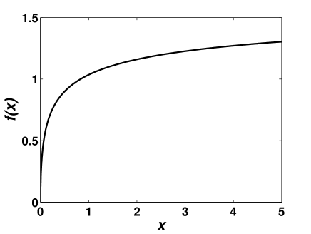
Figure 1: The scaling function $f(x).$

In one dimension, the scaling law dependence of the surface width at a scale $a$, involves integer exponents in the two cases, the EW Moktadir04 and the linear MBE equations, unlike the scaling exponents observed in the dependence with the system size, which are fractional. Table 1 summaries the value of exponents in both cases in one dimensional space.

	$\alpha$	z
EW	1(1/2)	2
MBE	2(3/2)	4

Table 1: Values of the exponents in the two cases: the EW equation and the linear MBE equation in one dimension. Between brackets are values of the exponents observed in the scaling with the system size.

II.2.2 Correlated noise

Similar to the above calculations, we will determine a different set of exponents by computing the surface width corresponding to each wavelet scale $a$ taking the substrate size infinite, in the case of spatially correlated noise. In this case the power spectrum is given by:

$$P_{\rho}(q)=2D_{\rho}q^{-2\rho}\frac{(1-\exp(-2q^{4}t))}{q^{4}}$$ (18)

We have for the surface width at the scale $a$:

$$\sigma_{\rho}\left(a,t\right)^{2}=2a^{5}D_{\rho}\pi\int_{0}^{\infty}{{q}^{-2\rho}\left(1-{e^{-2q^{4}t}}\right)e^{-{a}^{2}{q}^{2}}}{dq}$$ (19)

In this integration we have taken the upper cutoff to be infinite. By simple change of variable we have:

$$\sigma_{\rho}\left(a,t\right)^{2} = \pi D_{\rho}a^{4+2\rho}\int_{0}^{\infty}\xi^{-\rho-1/2}(1-e^{-2\xi^{2}t/a^{4}})e^{-\xi}d\xi$$ (20)

$$\propto a^{4+2\rho}f_{\rho}\left(\frac{t}{a^{4}}\right)^{2}$$

here, $f_{\rho}(x)^{2}=\int_{0}^{\infty}\xi^{-\rho-1/2}(1-e^{-2\xi^{2}x})e^{-\xi}d\xi$ is a scaling function which has the limit $f_{\rho}(x)\approx\sqrt{x}$ for $x<<1$ and $f_{\rho}(x)\approx\sqrt{\Gamma(1/2-\rho)}$, for $x>>1$, where $\Gamma$ is the gamma function. The result for the uncorrelated case is retrieved for $\rho=0$. Thus, for correlated noise, the roughness exponent is $\alpha(\rho)=2+\rho$ while $z=4$, independent of $\rho$. For the EW growth model, the roughness exponent was found to be $\alpha_{EW}=1+\rho$ Moktadir05 .

II.3 application to a computer model of the linear MBE

In this section we will apply the results obtained above to a computer model that simulate the linear molecular beam epitaxy in the case of uncorrelated noise. This model was developed in Krug94 to simulate the linear MBE growth. In this model, atoms are randomly deposited on a linear substrate and undergo a diffusion to neighboring sites in order to maximize their curvature $\kappa$. If the height at a site $i$ is $h(i)$, then the deposited atom at this site will move to a site $j$ with the maximum value of $\kappa=h_{j+1}-2h_{j}+h_{j-1}$. The diffusion length $l$ is such that $i-l\leq j\leq i+l$. Simulation is carried out for $l=2$ and a substrate size of $L=10^{6}$ sites.

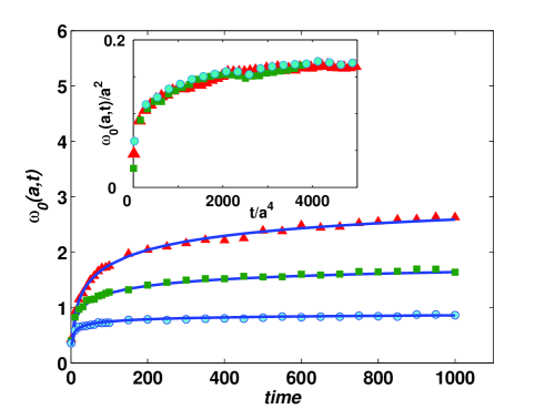
Figure 2: Computer simulation results showing the evolution of the surface width for three different scales a=2 $(\bullet)$, a=3 $(\blacksquare)$ and a=4 $(\blacktriangle)$. Full lines are the fit to the analytical expression (17). The inset shows the data collapse to a single curve confirming dynamic scaling form (17).

In figure 2 we show the plot of the surface width calculated at wavelet scales $a=$2,3 and 4 by performing the wavelet transform of the simulated profile and by using the expression $\sigma(a,t)=\left<(T(a,i)-\overline{T}(a))^{2}\right>_{i}$ where $\overline{T}(a)$ is the spatial average of $T(a,i)$, $i=1..N$. As can be seen, there is an excellent agreement between the simulated value of $\sigma(a,t)$ and the scaling form (17). The inset of figure 2 shows a good data collapse confirming the scaling form (17).

III Growth with Ehrlich$-$Schwoebel barrier

The current form $j_{m}$ in (I) represents a continuous uphill current leading to a slope selection i.e the mounds slope converges to a constant value $m_{0}$. This current is countered by the diffusion current $j_{d}$ preventing an indefinite increase of the mounds height. A simple linear stability analysis of (1) shows that this growth process is unstable against small perturbations with wavenumbers smaller than a critical value $k_{c}=\sqrt{\nu/K}$. This implies that the initial growth stage is characterized by the formation of mounds on the surface with the typical size $\lambda=2\pi\sqrt{2}/q_{c}$. After this initial phase, non-linearities become relevant triggering the coarsening of mounds. The scaling hypothesis implies that the coarsening behaviour is statistically self-similar i.e. surface mounds are similar in time domain up to a scaling by the average mound size $\lambda$. Under the scaling hypothesis, structure functions such as the height-height correlation function can be writing as $C(r)=\sigma(t)^{2}\theta(r/\lambda(t))$, where $\sigma$ is the surface width and $\theta$ is a scaling function. The evolution of $\lambda$ and $\sigma$ is expressed as:

$$\lambda \sim t^{n}$$

$$\sigma \sim t^{\beta}$$ (21)

The current form given by (I) leads to slope selection and the value of the scaling exponent $n=\frac{1}{3}$ Politi2002 .
We will show in the following, that the coarsening process can be well characterized by wavelets formalism. The advantage of this formalism is that one can track the coarsening in both, scale (or frequency) and the spatial position simultaneously. In addition we can quantify the coarsening we determine the evolution of a quantity called the scalegramMoktadir04 which is the counterpart of the power spectrum in Fourier analysis.

We first start by solving (1) numerically. The wavelet transform of the generated profiles is then computed at different times. The wavelet’s power spectrum is defined as the squared magnitude of the wavelet transform which is the analog of the power spectrum in Fourier analysis. Figure 3 displays the time evolution of the wavelet power spectrum at $t=100$, 500 and 1000 for $\nu/K=2$ and $N=500$; the result is averaged over 100 independent runs. The Hermitian wavelet of order 1 is used in these calculations. We can clearly notice the pattern formed at the early stage of growth where the power is concentrated around the dominant scale as a result of the linear instability. As time advances, the power shifts and spreads through higher scales, indicating the coarsening process.
In general, the mounds coarsening is characterized by the determination of the lateral correlation length or by determining the wavenumber corresponding to the maximum of the Fourier power spectrum. The latter is related to the mound size $\lambda$ via the relation $q_{max}=2\pi/\lambda$. One can efficiently characterize the coarsening process by performing the calculation of the the scalegramMoktadir04 . The scalegram is the spatial average of the wavelet power spectrum:

$$S(a,t)=<|T(a,x,t)|^{2}>_{x}$$ (22)

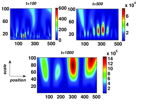
Figure 3: Color map plots showing the time evolution of the wavelet’s power spectrum of the evolving profile for three different times $t=100$, 500 and 1000. The early stage ($t=100$) shows the power concentration in a small band of scales surrounding the dominant scale as a result of linear instability. As time advances, this power is spread through larger scales as a result of the coarsening of mounds. The color scale is in arbitrary units.

The main advantage of the scalegram over the Fourier power spectrum is the fact that only few realizations are required to obtain an accurate scalegram. We can show that the scalegram defines a dominant scale at which it reaches its maximum value. We can obtain an analytical form of $S$ as a function of the scale $a$ and the mound size $\lambda=\lambda(t)$. Using the wavelet definition (6) we have:

$$S(a) = a^{2}\int\!\!\!\int\!<h(x+\xi a)h(x+\zeta a)>_{x}\psi(\xi)\psi(\zeta){d\xi}\,{d\zeta}$$ (23)

$$= a^{2}\int\int C(\xi,\zeta,a)\psi(\xi)\psi(\zeta){d\xi}\,{d\zeta}$$

The kernel $C(\xi,\zeta,a)\equiv<h(x+\xi a)h(x+\zeta a)>$ is the two points correlation function which depends only on the difference $\mid(\xi-\zeta)a\mid$ for the present process, that is: $C(\xi,\zeta,a)=C(\mid(\xi-\zeta)a\mid)$. We will choose the following form for $C(r)$Zhao98 :

$$C(r)=\sigma^{2}\exp\left(-\frac{r^{2}}{l^{2}}\right)\cos\left(\frac{2\pi r}{\lambda}\right)$$ (24)

where $\sigma$ is the surface width and $l$ is a parameter characterizing the decay of the correlations. The lateral correlation length is defined as $C(r)=\sigma^{2}/e$ and it is a function of both $l$ and $\lambda$. To obtain a simple analytical form of $S$, we use the Hermitian wavelet of order 1 ( $\psi(x)=-x\exp(-x^{2}/2)$. Integrating (23) in $(-\infty,+\infty)$ and using (24), we have:

$$S(a)=f(a,\lambda,l)\exp\left(-\frac{4\pi^{2}a^{2}l^{2}}{(4a^{2}+\l^{2})\lambda^{2}}\right)$$ (25)

Where:

$$f(a,\lambda,l)=\frac{4\pi a^{4}\sigma^{2}l(2\pi^{2}l^{4}+l^{2}\lambda^{2}+4a^{2}\lambda^{2})}{\lambda^{2}(4a^{2}+l^{2})^{5/2}}$$ (26)

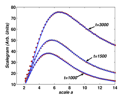
Figure 4: Plots of the scalegram obtained by numerical simulation(see text) at three different time $t=$1000, 1500 and 3000. Continuous lines are fits to the analytical form (25).

We determined the scalegram from numerical simulations of (1) by computing the wavelet transform of the obtained profile and using the definition (22). Figure 4 shows the results at three different times $t=$1000, 1500 and 3000. The Hermitian wavelet of order 1 was used with a system size of $N=500$. The ratio $\nu/K$ was set to 1.5, and the result was averaged over 100 independent runs. As can be seen, the agreement between numerical solution and the analytical form of the scalegram is extremely good. Equation (25) predicts the existence of a dominant scale $a^{*}$, which maximizes $S$, proportional to $\lambda$. Thus, the dominant scale evolves following the same power law followed by $\lambda$ i.e. (III).

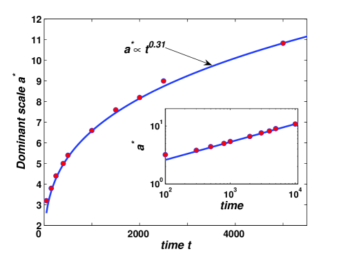
Figure 5: The evolution of the dominant scale (corresponding to the maximum of the scalegram) obtained from numerical simulations, showing a power law scaling with an exponent $n\simeq 1/3$. The inset shows the same result in a log-log plot.

This result is not surprising since the continuous wavelet transform gives the information on to what extent the frequency content of the analyzed profile, in the neighborhood of an arbitrary position $x$, is close to the frequency content of the wavelet at a given scale. To check the validity of the above we numerically computed the value of the dominant scale as a function of time. This is shown in figure 5. The power law nonlinear regression fit is also shown with an exponent $n=0.31\pm 0.01$, a value consistent with the coarsening exponent $n=1/3$ . A log-log plot of the result is also displayed at the inset of figure 5 confirming the power law scaling.

IV conclusion

In conclusion we investigated the epitaxial growth using wavelets formalism. Two cases were considered: the linear case where only atomic diffusion is the dominant process and the case where both atomic diffusion and Ehrlich$-$Schwoebel barrier are the dominant processes. In the former case, the linear equation is decomposed using a wavelet filter, allowing the discrimination of growth dynamics at each scale. We determined the scaling functions of the width corresponding to each wavelet decomposition of the surface profile, in two cases: growth with uncorrelated noise and growth with correlated noise. Analytical results were compared to a computer model simulating the linear growth in the case of uncorrelated noise. A good agreement was found between theory and computer simulation.
Growth incorporating ES effect alongside atomic diffusion is characterized by numerically computing the wavelet power spectrum. Coarsening process is quantified by the so called the scalegram, which revealed a time dependent dominant scale where the scalegram reaches its maximum. The dominant scale is proportional to the mound size i.e. following a power law with an exponent $n\simeq 1/3$. An analytical form of the scalegram is determined as a function of the scale and the mound size. This analytical form was compared to numerical results showing a good agreement between the two.

References

- (1) J. Krug 1999 Physica A 263 170
- (2) J. Krug 2002 Physica A 313 47
- (3) P. Politi, G. Grenet, A. Marty, A. Ponchet and J. Villain 2000 Physics Reports 324 271
- (4) A. Torcini and P. Politi 2002 Eur. Phys. J. B 25 519
- (5) M. Siegert and M. Plischke 1994 Phys. Rev. Lett. 73 517
- (6) M. Kalf, P. Smilauer, G. Comsa and T. Michely 1999 Surf. Sci. 426 L447
- (7) J.E. Van Nostrand, S.J. Chey, M.-A. Hasan, D.G. Cahill and J.E. Greene 1995 Phys. Rev. Lett. 74 1127
- (8) J.W. Evansa, P.A. Thiel and M.C. Bartelt 2006 Surf. Sci. Rep. 61 1
- (9) G. Ehrlich, F. Hudda 1966 J. Chem. Phys. 44 1039
- (10) W.W. Mullins 1957 J. Appl. Phys. 28 333
- (11) P. Politi and J. Villain 1996 Phys. Rev. B 54 5114
- (12) P. Politi and J. Villain 1997 Surface Diffusion: Atomistic and Collective Processes Ed M.C. Tringides (Plenum Press, New York) pp. 177
- (13) A. Pimpinelli and J. Villain 1998 Physics of crystal growth (Cambridge University press)
- (14) A. J. Bray 1994 Adv. Phys. 43 357
- (15) P. Politi 1998 Phys. Rev. E 58 281
- (16) I. Daubechis 2000 Ten Lectures on Wavelets CBMS, NSF Series in Applied Mathematics (SIAM, Philadelphia)
- (17) Z. Moktadir 2004 Phys. Rev. E 70 011602
- (18) J. Lawalle 1997 Phys. Rev. E 55 1590
- (19) J. Lawalle 1994 Acta Mech. 104 1
- (20) Z. Moktadir 2005 Phys. Rev. E 72 011608
- (21) J. Krug 1994 Phys. Rev. Lett. 72 2907
- (22) Y.-P. Zhao, H.-N. Yang, G.-C. Wang and T.-M. Lu 1998 Phys. Rev. B 57 1922