Disorder-dominated phases of random systems :
relations between tails exponents and scaling exponents

Abstract

We consider various random models (directed polymer, ferromagnetic random Potts model, Ising spin-glasses) in their disorder-dominated phases, where the free-energy cost $F(L)$ of an excitation of length $L$ present fluctuations that grow as a power-law $\Delta F(L)\sim L^{\omega}$ with the so-called droplet exponent $\omega>0$. We study the tails of the probability distribution $\Pi(x)$ of the rescaled free-energy cost $x=\frac{F_{L}-\overline{F_{L}}}{L^{\omega}}$, which are governed by two exponents $(\eta_{-},\eta_{+})$ defined by $\ln\Pi(x\to\pm\infty)\sim-|x|^{\eta_{\pm}}$. The aim of this paper is to establish simple relations between these tail exponents $(\eta_{-},\eta_{+})$ and the droplet exponent $\omega$. We first prove these relations for disordered models on diamond hierarchical lattices where exact renormalizations exist for the probability distribution $\Pi(x)$. We then interpret these relations via an analysis of the measure of the rare disorder configurations governing the tails. Our conclusion is that these relations, when expressed in terms of the dimensions of the bulk and of the excitation surface are actually valid for general lattices.

I Introduction

To understand the low-temperature phase of disordered systems, it is important to characterize both the statistics of the ground state energy over the disordered samples, and the statistics of excitations above the ground state within one sample.

The ground-state energy $E_{0}$ of a disordered sample is the minimal energy among the energies of all possible configurations. The study of its distribution thus belongs to the field of extreme value statistics. Whereas the case of independent random variables is well classified in three universality classes [1], the problem for the correlated energies within a disordered sample remains open and has been the subject of many recent studies. The interest lies both
(i) in the scaling behavior of the average $E_{0}^{av}(L)$ and the standard deviation $\Delta E_{0}(L)$ with the linear size $L$
(ii) in the asymptotic distribution $P(x)$ of the rescaled variable $x=(E_{0}-E_{0}^{av}(L))/\Delta E_{0}(L)$ in the limit $L\to\infty$

$${\cal P}_{L}(E_{0})\mathop{\simeq}_{L\to\infty}\frac{1}{\Delta E_{0}(L)}\ \Pi\left(x=\frac{E_{0}-E_{0}^{av}(L)}{\Delta E_{0}(L)}\right)$$ (1)

For spin-glasses in finite dimension $d$, a sample of linear size $L$ contains $N=L^{d}$ spins. Following the definitions of Ref. [2], the ‘shift exponent’ $\omega_{s}$ governs the correction to extensivity of the averaged value

$$E_{0}^{av}(L)\sim L^{d}e_{0}+L^{\omega_{s}}e_{1}+...$$ (2)

Within the droplet theory [3, 4], this shift exponent $\omega_{s}$ coincides with the domain wall exponent $\omega_{DW}$ and with the droplet exponent $\omega$ of low energy excitations (see below)

$$\omega_{s}=\omega_{DW}=\omega$$ (3)

The ‘fluctuation exponent’ $\omega_{f}$ governs the growth of the standard deviation

$$\Delta E_{0}(L)\sim L^{\omega_{f}}$$ (4)

In any finite dimension $d$, it has been proven that the fluctuation exponent is $\omega_{f}=d/2$ [5]. Accordingly, the rescaled distribution $P(x)$ of Eq. (1) was numerically found to be Gaussian in $d=2$ and $d=3$ [2], suggesting some Central Limit theorem. In contrast with finite-dimensional spin-glasses where one needs to introduce two exponents $\omega_{s}$ and $\omega_{f}$, the directed polymer model [6] is characterized by a single exponent $\omega$ that governs both the correction to extensivity of the average $E_{0}^{av}(L)$ and the width $\Delta E_{0}(L)$

$$E_{0}^{av}(L) \sim Le_{0}+L^{\omega}e_{1}+...$$

$$\Delta E_{0}(L) \sim L^{\omega}e_{2}+...$$ (5)

This exponent also governs the statistics of low excitations within the droplet theory [4], as confirmed numerically [7]. In dimension $1+1$, this exponent is exactly known to be $\omega(d=1)=1/3$ [8, 9, 10, 11] and the corresponding rescaled distribution $\Pi(x)$ is related to Tracy-Widom distributions of the largest eigenvalue of random matrices ensembles [10, 11, 12].

Among disordered systems, the directed polymer model thus presents the following distinctive feature : the statistics of the ground state energy over the samples is directly related to the statistics of excitations within a given sample [4]. In finite-dimensional spin systems however, the statistics of the ground-state energy over the samples is not very interesting : the fluctuation exponent $\theta_{f}=d/2$ and the corresponding Gaussian distribution $P(x)$ simply reflects the fluctuations of the $L^{d}$ random couplings defining the samples. The only information it contains on the statistics of excitations is the shift exponent $\omega_{s}=\omega$ governing the correction to extensivity of the averaged value. In this paper, we will be interested into the statistics of the energy $E_{L}$ of excitations above the ground state in a given sample. Its fluctuations are governed by the droplet exponent $\omega$

$$\Delta E_{L}\sim L^{\omega}$$ (6)

and its distribution is expected to follow a scaling form as $L\to\infty$

$$P_{L}(E_{L})\mathop{\simeq}_{L\to\infty}\frac{1}{L^{\omega}}\ {\widetilde{\Pi}}\left(x=\frac{E_{L}-\overline{E_{L}}}{L^{\omega}}\right)$$ (7)

Our aim is to show that the exponents governing the tails of the rescaled distributions ${\widetilde{\Pi}}(x)$ are simply related to the droplet exponent $\omega$. Since the whole low-temperature phase ($T<T_{c}$) is described at large scale by the zero-temperature fixed point, the statistics of the free-energy $F_{L}$ of excitations at $T<T_{c}$ is the same as the statistics of the energy $E_{L}$ of excitations above the ground state, up to some rescaling with the correlation length $\xi(T)$. So the results concerning the tails of ${\widetilde{\Pi}}(x)$ also concerns the tails of the free-energy of excitations at any temperature $T<T_{c}$.

To establish the relations existing between the tails of the probability distribution ${\widetilde{\Pi}}(x)$ and the droplet exponent $\omega$, we will first focus on the diamond hierarchical lattices where exact renormalizations exist as we now recall. Among real-space renormalization procedures [13], Migdal-Kadanoff block renormalizations [14] play a special role because they can be considered in two ways, either as approximate renormalization procedures on hypercubic lattices, or as exact renormalization procedures on certain hierarchical lattices [15, 16]. One of the most studied hierarchical lattice is the diamond lattice which is constructed recursively from a single link called here generation $n=0$ (see Figure 1): generation $n=1$ consists of $b$ branches, each branch containing $2$ bonds in series ; generation $n=2$ is obtained by applying the same transformation to each bond of the generation $n=1$. At generation $n$, the length $L_{n}$ between the two extreme sites $A$ and $B$ is $L_{n}=2^{n}$, and the total number of bonds is

$$B_{n}=(2b)^{n}=L_{n}^{d_{Liens}(b)}\ \ \ {\rm\ \ with\ \ }d_{eff}(b)=\frac{\ln(2b)}{\ln 2}$$ (8)

where $d_{eff}(b)$ represents some effective dimensionality.

Figure 1: Hierarchical construction of the diamond lattice of branching ratio $b$.

On this diamond lattice, various disordered models have been studied, such as for instance the diluted Ising model [17], ferromagnetic random Potts model [18, 19, 20], spin-glasses [21, 22, 23, 24, 25] and the directed polymer model [26, 27, 28, 29, 30, 31, 32, 33, 34]. In this article, we start from the exact renormalizations existing for these disordered models on the diamond lattices to derive the relations existing between the tails exponents and the droplet exponent $\omega$.

The paper is organized as follows. The tails of the distribution $\Pi(x)$ of the ground state energy of the directed polymer are discussed in Section II together with numerical results; the tails of the distribution ${\widetilde{\Pi}}(x)$ of excitations in the ferromagnetic random Potts model and in the Ising spin-glasses are studied in Section III and in Section IV respectively. Finally in Section V, we generalize these results to other lattices via an analysis of the measure of the rare disorder configurations governing the tails. Our conclusions are summarized in Section VI. Appendix A contains more detailed calculations, and Appendix B contains a brief reminder of Zhang argument for the directed polymer on hypercubic lattices.

II Directed polymer on diamond lattice

In this Section, we study the tails of the rescaled probability distribution $\Pi(x)$ for the ground state energy of the directed polymer model. (Eq. 1).

II.1 Reminder on the exact renormalization

II.1.1 Renormalization at finite temperature

The model of a directed polymer in a random medium [6] can be defined on diamond hierarchical lattice with $b$ branches [26, 27, 28, 29, 30, 31, 32, 33, 34]. The partition function $Z_{n}$ of generation $n$ satisfies the exact recursion [27]

$$Z_{n+1}=\sum_{a=1}^{b}Z_{n}^{(2a-1)}Z_{n}^{(2a)}$$ (9)

where $(Z_{n}^{(1)},...,Z_{n}^{(2b)})$ are $(2b)$ independent partition functions of generation $n$. At generation $n=0$, the lattice reduces to a single bond with a random energy $\epsilon$ drown from some distribution $\rho(\epsilon)$ and thus the initial condition for the recursion of Eq. 9 is simply

$$Z_{n=0}=e^{-\beta\epsilon}$$ (10)

In the low-temperature phase where the free-energy width $\Delta F(L)$ grows with the scale $L$, the recursion is dominated at large scale by the maximal term in Eq. 9

$$Z_{n+1}\mathop{\simeq}max_{1\leq a\leq b}\left(Z_{n}^{(2a-1)}Z_{n}^{(2a)}\right)$$ (11)

or equivalently in terms of free-energies $F_{n}=-T\ln Z_{n}$

$$F_{n+1}\mathop{\simeq}min_{1\leq a\leq b}\left(F_{n}^{(2a-1)}+F_{n}^{(2a)}\right)$$ (12)

This effective low-temperature recursion coincides with the recursion of the energy $E_{0}$ of the ground state studied in [26, 27]. The whole low-temperature phase is thus described by the zero-temperature fixed-point.

II.1.2 Renormalization at zero temperature

We now focus on the statistics of the ground state energy of the directed polymer [26, 28, 29, 32]. At $T=0$, the recursion for the ground state energy involves the following minimisation [26]

$$E_{n+1}=min\left[E_{n}^{(1)}+E_{n}^{(2)};E_{n}^{(3)}+E_{n}^{(4)};...;E_{n}^{(2b-1)}+E_{n}^{(2b)}\right]$$ (13)

This translates into the following recursion for the probability $P_{n}(E)$ [26] :

$$\int_{z}^{+\infty}dEP_{n+1}(E)=\left[\int_{z}^{+\infty}dSQ_{n}(S)\right]^{b}$$ (14)

where $Q_{n}(S)$ is the distribution of the sum $S=E_{n}^{(1)}+E_{n}^{(2)}$

$$Q_{n}(S)=\int_{-\infty}^{+\infty}dE_{1}\int_{-\infty}^{+\infty}dE_{2}P_{n}(E_{1})P_{n}(E_{2})\delta(S-(E_{1}+E_{2}))$$ (15)

II.1.3 Renormalization in the scaling regime

For large $n$, one expects the scaling [26]

$$P_{n}(E)\mathop{\simeq}_{n\to\infty}\frac{1}{\delta_{n}}\Pi_{b}\left(\frac{E-\gamma_{n}}{\delta_{n}}\right)$$ (16)

where the term $\gamma_{n}$ is extensive in the length $L_{n}$

$$\gamma_{n}\mathop{\simeq}_{n\to\infty}e_{0}L_{n}$$ (17)

i.e. $\gamma_{n+1}/\gamma_{n}\to 2$. The width $\delta_{n}$ scales with the length $L_{n}$ with some a priori unknown exponent $\omega$ [26]

$$\delta_{n}\mathop{\simeq}\lambda^{n}\simeq L_{n}^{\omega}\ \ {\rm with\ \ }\lambda\equiv 2^{\omega}$$ (18)

Replacing the scaling form of Eq. 16 in the recursion of Eqs 14, 15 yields

$$\int_{\frac{z-\gamma_{n+1}}{\delta_{n+1}}}^{+\infty}dx\Pi_{b}(x)=\left[\int_{\frac{z-2\gamma_{n}}{\delta_{n}}}^{+\infty}dx\int_{-\infty}^{+\infty}dx_{1}\int_{-\infty}^{+\infty}dx_{2}\Pi_{b}(x_{1})\Pi_{b}(x_{2})\delta(x-(x_{1}+x_{2}))\right]^{b}$$ (19)

Using $\gamma_{n+1}/\gamma_{n}=2$ and $\delta_{n+1}/\delta_{n}\to\lambda=2^{\omega}$, one obtains

$$\int_{\frac{u}{\lambda}}^{+\infty}dx\Pi_{b}(x)=\left[\int_{u}^{+\infty}dxG_{b}(x)\right]^{b}$$ (20)

where

$$G_{b}(x)\equiv\int_{-\infty}^{+\infty}dx_{1}\int_{-\infty}^{+\infty}dx_{2}\Pi_{b}(x_{1})\Pi_{b}(x_{2})\delta(x-(x_{1}+x_{2}))$$ (21)

The recursion simplifies in the limit $b=1$, where it reduces to the Central Limit theorem for the sum of random variables with [26]

$$\omega(b=1) =\frac{1}{2}$$

$$\Pi_{b=1}(x) =\frac{1}{\sqrt{2\pi}}e^{-\frac{x^{2}}{2}}$$ (22)

We refer to [26] where an expansion in $b=1+\epsilon$ has been developed.

Another limit where the recursion simplifies is $b\to\infty$. In the limit, a single iteration consists in taking the minimum of a large number $b\to\infty$ of random variables. The rescaled distribution is then the Gumbel distribution [1]

$$\omega(b\to\infty) =0$$

$$\Pi_{b\to\infty}(x) =e^{x-e^{x}}$$ (23)

For $1<b<+\infty$, the exponent $\omega(b)$ is expected to decay from $\omega(b=1)=1/2$ to $\omega(b=\infty)=0$, Accordingly, the rescaled distribution $\Pi_{b}(x)$ is expected to interpolate between the Gaussian and the Gumbel distribution.

II.2 Relations between tails exponents and the droplet exponent

Let us now focus on the tail exponents $\eta(b)$ and $\eta^{\prime}(b)$ of the probability distribution $\Pi_{b}$

$$\ln\Pi_{b}(x) \mathop{\simeq}_{x\to-\infty}-c(-x)^{\eta(b)}+...$$

$$\ln\Pi_{b}(x) \mathop{\simeq}_{x\to+\infty}-dx^{\eta^{\prime}(b)}+...$$ (24)

From the two extreme cases of Eqs 22 and 23, one expects that the left exponent $\eta(b)$ varies between

$$\eta(b=1) =2$$

$$\eta(b=\infty) =1$$ (25)

whereas the right exponent $\eta^{\prime}(b)$ varies between

$$\eta^{\prime}(b=1) =2$$

$$\eta^{\prime}(b=\infty) =\infty$$ (26)

The aim of this section is to show that these tail exponents are simply related to the droplet exponent $\omega(b)$ via

$$\eta(b) =\frac{1}{1-\omega(b)}$$

$$\eta^{\prime}(b) =\frac{\ln(2b)}{\ln 2}\eta(b)$$ (27)

To make things clearer, we have chosen to present here in the text only simple saddle-point arguments at leading order. We refer to Appendix A (see Eqs 106 and 123) for a much more detailed proof with subleading corrections.

II.2.1 Left-tail exponent $\eta$

Assume that the left-tail decay of the probability distribution $\Pi_{b}(x)$ is given at leading order by Eq. 24. A saddle-point analysis shows that the probability distribution $G_{b}$ (Eq 21) of the sum $x=x_{1}+x_{2}$ presents the tail

$$\ln G_{b}(x)\mathop{\simeq}_{x\to-\infty}-2c\left(-\frac{x}{2}\right)^{\eta}+...$$ (28)

The recursion of Eq. 20 yields by differentiation that the tail of $\Pi_{b}$ is related to the tail of $G_{b}$ via

$$\frac{1}{\lambda}\Pi_{b}\left(\frac{u}{\lambda}\right)\mathop{\simeq}_{u\to-\infty}bG_{b}(u)\left[\int_{u}^{+\infty}dyG_{b}(y)\right]^{b-1}\mathop{\simeq}_{u\to-\infty}bG_{b}(u)\mathop{\propto}_{u\to-\infty}be^{-2c\left(-\frac{u}{2}\right)^{\eta}+...}$$ (29)

Using $\lambda=2^{\omega}$, this yields in terms of the variable $x=u/\lambda$

$$\ln\Pi_{b}\left(x\right)\mathop{\simeq}_{x\to-\infty}-2c\left(-\frac{\lambda x}{2}\right)^{\eta}+...=-2^{1+\eta(\omega-1)}c\left(-x\right)^{\eta}+...$$ (30)

The consistency with the scaling form of the tail of Eq 24 yields $\eta=1/(1-\omega)$ as stated in Eq 27.

II.2.2 Right-tail exponent $\eta^{\prime}$

Assume that the right-tail decay of the probability distribution $\Pi_{b}(x)$ is given at leading order by (Eq. 24). A saddle-point analysis shows that the probability distribution $G_{b}$ (Eq 21) of the sum $x=x_{1}+x_{2}$ presents the tail

$$\ln G_{b}(x)\mathop{\simeq}_{x\to+\infty}-2c\left(\frac{x}{2}\right)^{\eta^{\prime}}+...$$ (31)

The recursion of Eq. 20 yields by differentiation that the tail of $\Pi_{b}$ is related to the tail of $G_{b}$ via

$$\frac{1}{\lambda}\Pi_{b}\left(\frac{u}{\lambda}\right)\mathop{\simeq}_{u\to+\infty}bG_{b}(u)\left[\int_{u}^{+\infty}dyG_{b}(y)\right]^{b-1}\mathop{\propto}_{u\to-\infty}\left[G_{b}(u)\right]^{b}\mathop{\propto}_{u\to-\infty}e^{-2bc\left(-\frac{u}{2}\right)^{\eta^{\prime}}+...}$$ (32)

Using $\lambda=2^{\omega}$, this yields in terms of the variable $x=u/\lambda$

$$\ln\Pi_{b}\left(x\right)\mathop{\simeq}_{x\to-\infty}-2bc\left(-\frac{\lambda x}{2}\right)^{\eta^{\prime}}+...=-2^{1+\eta^{\prime}(\omega-1)}bc\left(-x\right)^{\eta^{\prime}}+...$$ (33)

The consistency with the scaling form of the tail of Eq 24 yields $\eta^{\prime}(1-\omega)=\ln(2b)/\ln 2$ as stated in Eq 27.

II.2.3 Discussion

The relations of Eq. 27 have already been found for the special case $b=2$ in [29]. However in [29], a third relation between the three exponents was also written, leading to the simple values $\eta(b=2)=3/2$ and $\eta^{\prime}(b=2)=3$ that seem now excluded numerically (see below).

II.3 Numerical results of the ground state energy statistics

II.3.1 Method : numerical recursion of the probability distribution

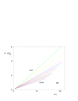
Figure 2: (Color online) Width $\Delta E_{0}(L)$ of the ground state energy distribution for a polymer of length $L$ (a) the log-log plot of width $\Delta E_{0}\sim L^{\omega(b)}$ for $b=2,3,4,5,6,7,8,12,16,24$. (b) Exponent $\omega(b)$ as a function of the branching ratio $b$ (Precise numbers are given in Table 1)

As explained in [26], it is more convenient numerically to consider the iteration of discrete probability distributions of the form

$$P_{n}(e)=\sum_{m=-\infty}^{+\infty}a_{n}(m)\delta_{e,m}$$ (34)

where the energy $e$ can take only integer values. This form is conserved via the recursion of Eq 13 that only involves summation of energies and choice of minimal value. The convolution step of Eq. 15 can be written as

$$Q_{n}(e)\equiv(P_{n}*P_{n})(e)=\sum_{m=-\infty}^{+\infty}b_{n}(m)\delta_{e,m}$$ (35)

with the following rules

$$b_{n}(m)=\sum_{m^{\prime}=-\infty}^{+\infty}a_{n}(m^{\prime})a_{n}(m-m^{\prime})$$ (36)

Since the function

$$\int_{x}^{+\infty}deQ_{n}(e)=\sum_{m>x}b_{n}(m)=\sum_{m=-\infty}^{+\infty}c_{n}(m)\theta(m-1<x<m)$$ (37)

is constant on intervals with values

$$c_{n}(m)=\sum_{m^{\prime}=m}^{+\infty}b_{n}(m^{\prime})$$ (38)

it is easy to raise it to power $b$

$$\left[\int_{x}^{+\infty}deQ_{n}(e)\right]^{b}=\sum_{m^{\prime}=-\infty}^{+\infty}\left[c_{n}(m)\right]^{b}\theta(m-1<x<m)$$ (39)

Since we have

$$\int_{x}^{+\infty}deP_{n+1}(e)=\sum_{m>x}a_{n+1}(m)=\sum_{m^{\prime}=-\infty}^{+\infty}\left[\sum_{m^{\prime}=m}^{+\infty}a_{n+1}(m^{\prime})\right]\theta(m-1<x<m)$$ (40)

the recursion of Eq. 14 yields

$$\sum_{m^{\prime}=m}^{+\infty}a_{n+1}(m^{\prime})=\left[c_{n}(m)\right]^{b}$$ (41)

and thus the coefficients at generation $(n+1)$ can be obtained via

$$a_{n+1}(m)=\left[c_{n}(m)\right]^{b}-\left[c_{n}(m+1)\right]^{b}$$ (42)

This method allows to obtain very accurate results for the fluctuation exponent $\omega(b)$ and for the tail exponents $\eta(b)$ and $\eta^{\prime}(b)$ because the probability distribution can be evaluated very far in the tails. The results presented below have been obtained by the iteration up to $n_{g}\sim 30$ generations of the discrete distribution of Eq. 34 with numerical tail cut-offs of order $-10000\leq m-m_{center}(n)\leq 1000$ around the moving center $m_{center}(n)$ for each generation $n$.

II.3.2 Numerical results for the fluctuation exponent $\omega(b)$

b $\ \ \omega(b)$ $\ \ \eta(b)$ 2 0.299 1.43 3 0.236 1.31 4 0.205 1.26 5 0.186 1.23 6 0.173 1.21 7 0.163 1.20 8 0.156 1.18 12 0.141 1.16 16 0.131 1.15 24 0.123 1.14

Table 1: Results for the exponents $\omega(b)$ and $\eta(b)$ as the number $b$ of branches varies

We first show on Fig. 2 the log-log plot of width $\Delta E_{0}\sim L^{\omega(b)}$ of the ground state energy probability distribution. The measures of the slopes yield the values given in Table 1. The values of $\omega(b)$ are in agreement with the existing previous numerical measures [26, 28, 29, 32]. The curve $\omega(b)$ shown on Fig. 2 b seems to suggest that the droplet exponent $\omega$ remains positive as long as the effective dimension $d_{eff}(b)=\ln(2b)/\ln 2$ (Eq 8) remains finite. Note that for hypercubic lattices, the existence of a finite upper critical dimension $d_{c}$ above which the droplet exponent vanishes has remained a very controversial issue between the numerical studies [35, 36, 37, 38] and various theoretical approaches [39, 40, 41].

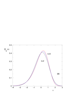
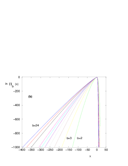
Figure 3: (Color online) Rescaled probability distribution of the ground state energy (a) Bulk representation for $b=2,4,8$ (b) Log plot for $b=2,3,4,5,6,7,8,12,16,24$ to see the behavior far in the tails

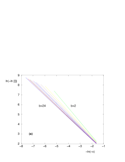
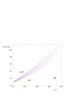
Figure 4: (Color online) Log-log plot of the tails of the rescaled probability distribution of the ground state energy for branching ratio $b=2,3,4,5,6,7,8,12,16,24$. (a) Measure of the exponent $\eta(b)$ governing the left tail $\ln\Pi_{b}(x\to-\infty)\sim-(-x)^{\eta(b)}$ (b) Measure of the exponent $\eta^{\prime}(b)$ governing the right tail $\ln\Pi_{b}(x\to+\infty)\sim-x^{\eta^{\prime}(b)}$ The curvatures of $\ln(-\ln\Pi_{b}(x))$ as a function of $\ln(x)$ show that the corrections to the leading behavior are stronger than for the left tail shown in (a).

II.3.3 Numerical results for the rescaled probability distribution $\Pi_{b}(x)$

We show on Fig. 3 the asymptotic rescaled probability distributions $\Pi_{b}(x)$ defined in Eq. 1. On Fig. 3 (a) we show $\Pi_{b}(x)$ in the bulk for $b=2,4,8$. On Fig. 3 (b) we show $\ln\Pi_{b}(x)$ to see the behaviors far in the tails.

From the Figures 4, we have measured the tails exponents defined by Eq. 24. The left-tail exponent $\eta(b)$ can be measured as the slopes of the curves of Fig. 4 (a). The results $\eta(b)$ are given in Table 1. The relation $\eta(b)=1/(1-\omega(b))$ (Eq. 27) is well satisfied by our numerical results.

The right-tail exponent $\eta^{\prime}(b)$ turns out to be more difficult to measure precisely, because the corrections to the leading behavior are much stronger, as shown by the curvatures of our results of Fig. 4 (b). However, the values predicted by the relation of Eq. 27

$$\eta^{\prime}(b)=\frac{\ln(2b)}{\ln 2}\ \eta(b)$$ (43)

are compatible with our data.

II.4 Extension to the critical point

On the diamond hierarchical lattice, the free-energy fluctuations of the directed polymer either grow as $L^{\omega}$ for $T<T_{c}$, or decay as $L^{-\omega^{\prime}}$ for $T>T_{c}$ or remain of order $O(1)$ exactly at $T_{c}$. The study of the tails of the critical rescaled distribution [42] is a special case of the above relations (Eq 27) with $\omega_{c}=0$

$$\eta_{c}(b) =1$$

$$\eta^{\prime}_{c}(b) =\frac{\ln(2b)}{\ln 2}$$ (44)

We refer to [42] for more details.

III Ising and Potts random ferromagnets on diamond lattice

In this section, we study the tails of the rescaled distribution ${\widetilde{\Pi}}(x)$ for the excitations in random Ising and Potts ferromagnets (Eq. 7).

III.1 Reminder on the exact renormalization for the effective coupling

The Ising Hamiltonian reads

$$H_{Ising}=-\sum_{<i,j>}J_{i,j}S_{i}S_{j}$$ (45)

where the spins take the values $S_{i}=\pm 1$ and where the couplings $J_{i,j}$ are positive random variables (see below section IV on spin-glass for couplings of random sign). The Potts Hamiltonian is a generalization where the variable $\sigma_{i}$ can take $q$ different values.

$$H_{Potts}=-\sum_{<i,j>}2J_{i,j}\delta_{\sigma_{i},\sigma_{j}}$$ (46)

(We choose $(2J)$ to recover Ising for $q=2$)

III.1.1 Renormalization at finite temperature

The effective coupling between the two end-points $A$ and $B$ of the diamond lattice of Fig. 1 is defined by

$$e^{-2\beta J_{eff}}=\frac{Z_{+-}}{Z_{++}}=e^{-\beta\left(F_{+-}-F_{++}\right)}$$ (47)

where $Z_{++}$ and $Z_{+-}$ are the partitions functions corresponding respectively to the same color at both ends or to two different colors at both ends. So the effective coupling represents the free-energy cost of creating an interface between the two ends at distance $L$. The renormalization equation reads in terms of the variable $y=e^{2\beta J}$ [18, 19, 20]

$$y_{n+1}=\prod_{i=1}^{b}\left(\frac{y_{n}^{(i_{1})}y_{n}^{(i_{2})}+(q-1)}{y_{n}^{(i_{1})}+y_{n}^{(i_{2})}+(q-2)}\right)$$ (48)

In the low-temperature phase where the effective couplings $J_{n}$ grow with the length $L_{n}=2^{n}$, the contribution of each branch $(i)$ is dominated by the minimal coupling between $(J_{n}^{(i_{1})},J_{n}^{(i_{2})})$. This leads to the effective zero-temperature recursion

$$J_{n+1}\mathop{\simeq}\sum_{i=1}^{b}{\rm min}\left[J_{n}^{(i_{1})},J_{n}^{(i_{2})}\right]$$ (49)

The whole low-temperature phase is thus described by the zero-temperature fixed-point.

III.1.2 Renormalization at zero temperature

We now focus on the zero-temperature renormalization

$$J_{n+1}=\sum_{i=1}^{b}{\rm min}\left[J_{n}^{(i_{1})},J_{n}^{(i_{2})}\right]$$ (50)

Note that two operations ’sum’ and ’min’ occur in the opposite order with respect to the directed polymer case of Eq. 13. Eq. 50 translates into the following recursion for the probability $P_{n}(J)$ :

$$P_{n+1}(J)=\int_{0}^{+\infty}dK_{1}P_{n}^{min}(K_{1})...\int_{0}^{+\infty}dK_{b}P_{n}^{min}(K_{b})\delta(J-(K_{1}+K_{2}+...+K_{b}))$$ (51)

where $P_{n}^{min}(K)$ is the distribution of the minimum $K=min(J_{n}^{(1)},J_{n}^{(2)})$ of two variables drawn with the distribution $P_{n}(J)$

$$\int_{z}^{+\infty}dKP_{n}^{min}(K)=\left[\int_{z}^{+\infty}dJP_{n}(J)\right]^{2}$$ (52)

III.1.3 Renormalization in the scaling regime

For large $n$, one expects the scaling

$$P_{n}(J)\mathop{\simeq}_{n\to\infty}\frac{1}{L_{n}^{\omega}}{\widetilde{\Pi}}_{b}\left(\frac{J-\gamma_{n}}{L_{n}^{\omega}}\right)$$ (53)

Replacing the scaling form of Eq. 53 in the recursion of Eqs 51, 52 yields

$$\frac{1}{\lambda}{\widetilde{\Pi}}_{b}\left(\frac{u}{\lambda}\right)=\int_{-\infty}^{+\infty}dx_{1}{\widetilde{\Pi}}_{b}^{min}(x_{1})...\int_{-\infty}^{+\infty}dx_{b}{\widetilde{\Pi}}_{b}^{min}(x_{b})\delta(u-(x_{1}+x_{2}+...+x_{b}))$$ (54)

and

$$\int_{z}^{+\infty}dx{\widetilde{\Pi}}_{b}^{min}(x)=\left[\int_{z}^{+\infty}dx{\widetilde{\Pi}}_{b}(x)\right]^{2}$$ (55)

and where the term $\gamma_{n}$ should grow asymptotically as $\gamma_{n+1}/\gamma_{n}\to b$. In terms of the effective dimension $d_{eff}(b)$ of Eq 8, this corresponds to

$$\gamma_{n}\sim b^{n}=L_{n}^{\frac{\ln b}{\ln 2}}=L_{n}^{d_{eff}(b)-1}$$ (56)

as it should for an interface of dimension $d_{s}=d_{eff}(b)-1$.

The recursion simplifies in the limit $b\to\infty$ [23] where a single iteration consists in summing a large number of random variables

$${\widetilde{\Pi}}_{b\to\infty}(x)=\frac{1}{\sqrt{2\pi}}e^{-\frac{x^{2}}{2}}$$ (57)

(Note that here, the usual other simple limit $b=1$ is not interesting since it does not correspond to a positive droplet exponent).

III.2 Relation between the tail exponents and the droplet exponent

Let us now focus on the tail exponents $\eta(b)$ and $\eta^{\prime}(b)$ of the probability distribution ${\widetilde{\Pi}}_{b}$ defined as in Eq 24. The aim of this section is to show that these tail exponents are simply related to the droplet exponent $\omega(b)$ via

$$\eta(b) =\frac{\frac{\ln b}{\ln 2}}{\frac{\ln b}{\ln 2}-\omega(b)}$$

$$\eta^{\prime}(b) =\frac{\frac{\ln(2b)}{\ln 2}}{\frac{\ln b}{\ln 2}-\omega(b)}$$ (58)

As in the directed polymer case, these relations can be obtained via simple saddle-point arguments.

III.2.1 Left-tail exponent $\eta$

If the left tail of ${\widetilde{\Pi}}_{b}(x)$ is described by Eq 24, the distribution ${\widetilde{\Pi}}_{b}^{min}$ presents the same decay by differentiation of Eq. 55

$${\widetilde{\Pi}}_{b}^{min}(x)=2{\widetilde{\Pi}}_{b}(x)\int_{x}^{+\infty}dy{\widetilde{\Pi}}_{b}(y)\mathop{\simeq}_{x\to-\infty}2{\widetilde{\Pi}}_{b}(x)\mathop{\simeq}_{x\to-\infty}2e^{-c(-x)^{\eta}}$$ (59)

A saddle-point analysis shows that the convolution of $b$ variables $K_{i}$ then presents the following decay (Eq 54)

$$\frac{1}{\lambda}{\widetilde{\Pi}}_{b}\left(\frac{u}{\lambda}\right)\mathop{\simeq}_{u\to-\infty}e^{-bc\left(-\frac{u}{b}\right)^{\eta}}$$ (60)

Using $\lambda=2^{\omega}$, this yields in terms of the variable $x=u/\lambda$

$$\ln{\widetilde{\Pi}}_{b}\left(x\right)\mathop{\simeq}_{x\to-\infty}-bc\left(-\frac{\lambda x}{b}\right)^{\eta}\mathop{\simeq}_{x\to-\infty}-b^{1-\eta}2^{\eta\omega}c(-x)^{\eta}$$ (61)

The consistency with the tail of Eq 24 yields the following constraint $2^{\eta\omega}=b^{\eta-1}$ leading to the result for $\eta(b)$ given in Eq 58.

III.2.2 Right-tail exponent $\eta^{\prime}$

If the right tail of ${\widetilde{\Pi}}_{b}(x)$ is described by Eq 24, the distribution ${\widetilde{\Pi}}_{b}^{min}$ presents the following exponential decay by differentiation of Eq. 55

$${\widetilde{\Pi}}_{b}^{min}(x)=2{\widetilde{\Pi}}_{b}(x)\int_{x}^{+\infty}dy{\widetilde{\Pi}}_{b}(y)\mathop{\propto}_{x\to+\infty}{\widetilde{\Pi}}_{b}^{2}(x)\mathop{\propto}_{x\to+\infty}e^{-2dx^{\eta^{\prime}}}$$ (62)

A saddle-point analysis shows that the convolution of $b$ variables $K_{i}$ then presents the following decay (Eq 54)

$$\frac{1}{\lambda}{\widetilde{\Pi}}_{b}\left(\frac{u}{\lambda}\right)\mathop{\simeq}_{u\to+\infty}e^{-2bd\left(\frac{u}{b}\right)^{\eta^{\prime}}}$$ (63)

Using $\lambda=2^{\omega}$, this yields in terms of the variable $x=u/\lambda$

$$\ln{\widetilde{\Pi}}_{b}\left(x\right)\mathop{\simeq}_{x\to+\infty}-2bd\left(\frac{\lambda x}{b}\right)^{\eta^{\prime}}\mathop{\simeq}_{x\to+\infty}-b^{1-\eta^{\prime}}2^{1+\eta^{\prime}\omega}dx^{\eta^{\prime}}$$ (64)

The consistency with the tail of Eq 24 yields the following constraint $2^{1+\eta^{\prime}\omega}=b^{\eta^{\prime}-1}$ leading to the result for $\eta^{\prime}(b)$ given in Eq 58.

III.3 Extension to the critical point

As in the directed polymer case (Eq 44), one may try to extend the results on the tail behaviors in the low-temperature phase where $\omega>0$ to the critical point where $\omega_{c}=0$. The right tail exponent becomes at criticality (Eq 58)

$$\eta_{c}^{\prime}(b) =\frac{\ln(2b)}{\ln b}$$ (65)

For the left tail however, the problem is qualitatively different at criticality and will not be discussed here ( the critical invariant distribution $P_{c}(J)$ does not extend to $(-\infty)$ anymore, but reaches the natural boundary $J=0$.)

IV Spin-glasses on diamond lattice

We now consider the case of Ising spin-glasses described by Eq. 45, but now the random couplings $J_{i,j}$ can be positive or negative and are distributed with a symmetric distribution $P_{0}(J)$

$$P_{0}(J)=P_{0}(-J)$$ (66)

IV.1 Reminder on the exact renormalization for the effective coupling

IV.1.1 Renormalization at zero temperature

The renormalization at finite temperature is still described by Eq. 48 with $q=2$. However, the fact that the couplings are of arbitrary sign yields that the zero-temperature renormalization now reads

$$J_{n+1}=\sum_{i=1}^{b}{\rm sign}\left(J_{n}^{(i_{1})}J_{n}^{(i_{2})}\right){\rm min}\left[|J_{n}^{(i_{1})}|,|J_{n}^{(i_{2})}|\right]$$ (67)

instead of Eq 50 corresponding to the case of positive couplings only. The symmetry of the initial condition (Eq 67) is conserved by the renormalization

$$P_{n}(J)=P_{n}(-J)$$ (68)

To translate the renormalization of Eq. 67 into a recursion for the probability distribution $P_{n}(J)$, it is convenient to introduce the probability distribution $P_{n}^{abs}$ of $|J_{n}|$

$$P_{n}^{abs}(J>0)=P_{n}(J)+P_{n}(-J)=2P_{n}(J)$$ (69)

and the probability distribution $Q_{n}^{abs}(K)$ of $K={\rm min}\left[|J_{n}^{(1)}|,|J_{n}^{(2)}|\right]\geq 0$ satisfying

$$\int_{z}^{+\infty}dKQ_{n}^{abs}(K)=\left[\int_{z}^{+\infty}dJP_{n}^{abs}(J)\right]^{2}$$ (70)

(the value $z=0$ corresponds to the normalization condition of both distribution). The probability distribution $Q_{n}(J)$ of $K={\rm sign}\left(J_{n}^{(1)}J_{n}^{(2)}\right){\rm min}\left[|J_{n}^{(1)}|,|J_{n}^{(2)}|\right]\geq 0$ is symmetric in $K\to-K$

$$Q_{n}(K\neq 0)=\frac{1}{2}Q_{n}^{abs}\left(|K|\right)$$ (71)

The recursion of Eq. 67 corresponds to the convolution

$$P_{n+1}(J)=\int_{-\infty}^{+\infty}dK_{1}Q_{n}(K_{1})...\int_{-\infty}^{+\infty}dK_{b}Q_{n}(K_{b})\delta(J-(K_{1}+K_{2}+...+K_{b}))$$ (72)

IV.1.2 Renormalization in the scaling regime

For large $n$, one expects the scaling

$$P_{n}(J)\mathop{\simeq}_{n\to\infty}\frac{1}{L_{n}^{\omega}}{\widetilde{\Pi}}_{b}\left(\frac{J}{L_{n}^{\omega}}\right)$$ (73)

where $\gamma_{n}=0$ in contrast with the ferromagnetic case of Eq 53, and where the scaling function ${\widetilde{\Pi}}_{b}$ is symmetric ( Eq. 68 )

$${\widetilde{\Pi}}_{b}(x)={\widetilde{\Pi}}_{b}(-x)$$ (74)

IV.2 Relation between the tail exponent and the droplet exponent

Note that the true rescaled distribution ${\widetilde{\Pi}}^{true}(x)$ as defined by Eq. 7 with a positive energy for excitations above the ground state actually corresponds to the distribution of the absolute value of the rescaled coupling ${\widetilde{\Pi}}_{b}(x)$ defined in Eq 73

$${\widetilde{\Pi}}^{true}_{b}(x)={\widetilde{\Pi}}_{b}(x)+{\widetilde{\Pi}}_{b}(-x)$$ (75)

So the true distribution ${\widetilde{\Pi}}^{true}_{b}(x)$ begins at $x=0$ with a non-zero value ${\widetilde{\Pi}}^{true}_{b}(0)$ [4] and there exists a single tail as $x\to+\infty$. So in contrast with the previous cases of the directed polymer and of the ferromagnetic Potts model described by two tail exponents (Eq 24), the distribution ${\widetilde{\Pi}}_{b}(x)$ of the rescaled coupling for spin-glasses presents a single exponent $\eta^{\prime}(b)$ as a consequence of the symmetry of Eq. 74

$$\ln{\widetilde{\Pi}}_{b}(x)\mathop{\simeq}_{x\to\pm\infty}-d|x|^{\eta^{\prime}}$$ (76)

We will not repeat here the calculations that are similar to the case of the right tail of the Potts model and that lead to the same relation between exponents (Eq 58)

$$\eta^{\prime}(b)=\frac{\frac{\ln(2b)}{\ln 2}}{\frac{\ln b}{\ln 2}-\omega(b)}$$ (77)

V Generalization of the tail exponents relations to other lattices

In the previous sections, we have derived the relations that exist between the tail exponents $(\eta,\eta^{\prime})$ and the scaling exponent $\omega$ for various disordered models on the diamond hierarchical lattices from the exact renormalization recursions. The obtained relations are actually very simple in terms of the effective dimension $d_{eff}(b)$ of these lattices (Eq. 8). This suggest that these relations should have a simple interpretation. In this section, we explain the physical meaning of these relations and generalize them to other lattices.

V.1 Tail exponents for the directed polymer

V.1.1 Physical interpretation of the left tail

The relation $\eta=1/(1-\omega)$ ( Eq. 27 ) derived previously from the exact renormalization on the diamond lattice can be interpreted as follows. The left tail of the ground state energy of the directed polymer corresponds to samples that leads to much lower energy than the average. Let us evaluate the probability to obtain a ground state energy $E_{0}=\gamma_{n}-aL_{n}$ extensively below the averaged value $\gamma_{n}$ of the scaling function of Eq. 16 with tail behavior described by Eq 24

$$P_{n}(E_{0}=\gamma_{n}-aL_{n})\simeq\frac{1}{L_{n}^{\omega}}\Pi_{b}\left(-a\frac{L_{n}}{L_{n}^{\omega}}\right)\mathop{\propto}_{L_{n}\to\infty}e^{-ca^{\eta}L_{n}^{\eta(1-\omega)}}$$ (78)

On the other hand, to obtain such a ground state energy $E_{0}=\gamma_{n}-aL_{n}$ extensively below the averaged value $\gamma_{n}$, it seems reasonable to ask that each bond of the ground state configuration of length $L$ should have an energy $\epsilon_{i}$ lower than the average, which happens with the exponentially small probability

$$\left[\int_{-\infty}^{..}d\epsilon\rho(\epsilon)\right]^{L}\sim e^{-cstL}$$ (79)

The identification of the length exponents in Eqs 78 and 79 yields

$$\eta(1-\omega)=1$$ (80)

which corresponds to the relation found for the diamond lattice ( Eq. 27). From this interpretation in terms of the rare disordered samples that govern the left tail of the ground state energy configuration, we expect that the relation of Eq 80 is actually valid on any lattice, and in particular for hypercubic lattices of $1+d$ dimensions. The relation is satisfied by the exact exponents in $1+1$ dimensions with $\omega=1/3$ [8, 9, 10, 11] and $\eta=3/2$ [10, 11, 12]. The relation of Eq 80 has been previously derived for hypercubic lattices via Zhang argument [6] (the argument is recalled in Appendix B for comparison) and has been checked numerically in [43] for $d=2,3$. However Zhang argument only concerns the left tail because it is based on the existence of a Lyapunov exponent for positive moments of the partition function. It cannot be extended easily to the right tail that would be in correspondence with negative moments. This is in contrast with the rare events analysis presented here that can be extended to the right tail as we now explain.

V.1.2 Physical interpretation of the right tail

The relation $\eta^{\prime}=d_{eff}(b)/(1-\omega)$ ( Eq. 27 ) derived previously from the exact renormalization on the diamond lattice can be interpreted as follows. The right tail of the ground state energy of the directed polymer corresponds to samples that leads to much higher energy than the average. Let us evaluate the probability to obtain a ground state energy $E_{0}=\gamma_{n}+aL_{n}$ extensively higher the averaged value $\gamma_{n}$ of the scaling function of Eq. 16 with tail behavior described by Eq 24

$$P_{n}(E_{0}=\gamma_{n}+aL_{n})\simeq\frac{1}{L_{n}^{\omega}}\Pi_{b}\left(a\frac{L_{n}}{L_{n}^{\omega}}\right)\mathop{\propto}_{L_{n}\to\infty}e^{-da^{\eta^{\prime}}L_{n}^{\eta^{\prime}(1-\omega)}}$$ (81)

On the other hand, to obtain such a ground state energy $E_{0}=\gamma_{n}+aL_{n}$ extensively higher the averaged value $\gamma_{n}$, it seems reasonable to ask that all $L^{d_{eff}}$ bonds of the lattice should have an energy $\epsilon_{i}$ higher than the average, which happens with the exponentially small probability

$$\left[\int_{...}^{+\infty}d\epsilon\rho(\epsilon)\right]^{L^{d_{eff}}}\sim e^{-cstL^{d_{eff}}}$$ (82)

The identification of the length exponents in Eqs 81 and 82

$$\eta^{\prime}(1-\omega)=d_{eff}$$ (83)

exactly corresponds to the relation found for the diamond lattice ( Eq. 27). From this interpretation in terms of the rare disordered samples, we expect that the relation of Eq 83 is actually valid on any lattice, and in particular for hypercubic lattices of $d_{eff}=1+d$ dimensions. The relation is satisfied by the exact exponents in $1+1$ dimensions with $\omega=1/3$ [8, 9, 10, 11] and $\eta^{\prime}=3$ [10, 11, 12].

V.2 Tail exponents for the ferromagnetic random Potts model

V.2.1 Physical interpretation of the left tail

The relation derived for the left tail of the Potts model on the diamond lattice (Eq 58) reads in terms of the effective dimension $d_{eff}(b)$ of Eq 8

$$\eta(b)=\frac{d_{eff}(b)-1}{d_{eff}(b)-1-\omega(b)}$$ (84)

We now propose the following physical interpretation. The left tail corresponds to samples that leads to much lower effective coupling than the average $\gamma_{n}\sim L_{n}^{d_{eff}(b)-1}$ (Eq. 56) Let us evaluate the probability to obtain an effective coupling $J=\gamma_{n}-aL_{n}^{d_{eff}(b)-1}$ extensively below the averaged value $\gamma_{n}$ of the scaling function of Eq. 53 with tail behavior described by Eq 24

$$P_{n}(J=\gamma_{n}-aL_{n}^{d_{eff}(b)-1})\simeq\frac{1}{L_{n}^{\omega}}{\widetilde{\Pi}}_{b}\left(-a\frac{L_{n}^{d_{eff}(b)-1}}{L_{n}^{\omega}}\right)\mathop{\propto}_{L_{n}\to\infty}e^{-ca^{\eta}L_{n}^{\eta(d_{eff}(b)-1-\omega)}}$$ (85)

On the other hand, to obtain such a low effective coupling $J=\gamma_{n}-aL_{n}^{d_{eff}(b)-1}$ extensively below the averaged value $\gamma_{n}$, it seems reasonable to ask that each bond of the interface of dimension $L^{d_{eff}(b)-1}$ should have a coupling $J_{i}$ lower than the average, which happens with the exponentially small probability

$$\left[\int_{0}^{..}dJP_{0}(J)\right]^{L^{d_{eff}(b)-1}}\sim e^{-cstL^{d_{eff}(b)-1}}$$ (86)

The identification of the length exponents in Eqs 85 and 86

$$\eta({d_{eff}(b)-1-\omega)}=d_{eff}(b)-1$$ (87)

exactly corresponds to the relation found for the diamond lattice ( Eq. 84).

V.2.2 Physical interpretation of the right tail

The relation derived for the left tail of the Potts model on the diamond lattice (Eq 58) reads in terms of the effective dimension $d_{eff}(b)$ of Eq 8

$$\eta^{\prime}(b)=\frac{d_{eff}(b)}{d_{eff}(b)-1-\omega(b)}$$ (88)

We now propose the following physical interpretation. The right tail corresponds to samples that leads to much higher effective coupling than the average $\gamma_{n}\sim L_{n}^{d_{eff}(b)-1}$ (Eq. 56) Let us evaluate the probability to obtain an effective coupling $J=\gamma_{n}+aL_{n}^{d_{eff}(b)-1}$ extensively above the averaged value $\gamma_{n}$ of the scaling function of Eq. 53 with tail behavior described by Eq 24

$$P_{n}(J=\gamma_{n}+aL_{n}^{d_{eff}(b)-1})\simeq\frac{1}{L_{n}^{\omega}}{\widetilde{\Pi}}_{b}\left(a\frac{L_{n}^{d_{eff}(b)-1}}{L_{n}^{\omega}}\right)\mathop{\propto}_{L_{n}\to\infty}e^{-da^{\eta^{\prime}}L_{n}^{\eta^{\prime}(d_{eff}(b)-1-\omega)}}$$ (89)

On the other hand, to obtain such a high effective coupling $J=\gamma_{n}+aL_{n}^{d_{eff}(b)-1}$ extensively above the averaged value $\gamma_{n}$, it seems reasonable to ask that all bonds of the sample of dimension $L^{d_{eff}(b)}$ should have a coupling $J_{i}$ higher than the average, which happens with the exponentially small probability

$$\left[\int_{..}^{+\infty}dJP_{0}(J)\right]^{L^{d_{eff}(b)}}\sim e^{-cstL^{d_{eff}(b)}}$$ (90)

The identification of the length exponents in Eqs 89 and 90

$$\eta^{\prime}({d_{eff}(b)-1-\omega)}=d_{eff}(b)$$ (91)

exactly corresponds to the relation found for the diamond lattice ( Eq. 88).

VI Conclusion

In this paper, we have studied the statistics of excitations of finite-dimensional random models (directed polymer, ferromagnetic random Potts model, Ising spin-glasses) in their low-temperature phase characterized by a positive droplet exponent $\omega>0$. We have shown that the tails of the rescaled probability distribution are characterized by two tails exponents $(\eta,\eta^{\prime})$ that are simply related to the droplet exponent $\omega$. We have first proved these relations on the diamond hierarchical lattices where exact renormalizations exist for the rescaled probability distribution. We have then given the physical meaning of these relations in terms of the measure of the rare disorder configurations governing the tails. This interpretation allows to understand the asymmetry $\eta<\eta^{\prime}$ because a ’good’ sample contributing to the left tail is a sample containing $L^{d_{s}}$ ’good’ random variables for an interface of dimension $d_{s}<d$, whereas a ’bad’ sample contributing to the right tail is a sample containing $L^{d}$ ’bad’ random variables for the bulk of dimension $d$. We have then argued that this physical interpretation means that the relations between the tails exponent $(\eta,\eta^{\prime})$ and the droplet exponent $\omega$ should actually remain true on arbitrary lattices when expressed in terms of the dimensions $(d_{s},d)$, namely

$$\eta =\frac{d_{s}}{d_{s}-\omega}$$

$$\eta^{\prime} =\frac{d}{d_{s}-\omega}$$ (92)

The directed polymer corresponds to the case of a linear object $d_{s}=1$ embedded in a space of total dimension $d$, whereas the ferromagnetic random Potts model corresponds to an interface of dimension $d_{s}=d-1$ in a space of dimension $d$. These two cases merge for the special case of a linear object $d_{s}=1$ embedded in a space of total dimension $d=2$, which is not surprising since the directed polymer model was precisely invented to model a one-dimensional interface in two-dimensional ferromagnetic spin models at low temperature [44]. This special case also explains why it is the distribution of the ground state energy of the directed polymer model (Eq. 1) which is in direct correspondence with the distribution of excitations in ferromagnetic spin models (Eq. 7).

The case of spin-glasses is different for at least two reasons. First of all, only the right tail exponent $\eta^{\prime}$ exists, because the distribution of the energy of excitations extends down to $E=0$ as a consequence of the symmetry $J\to-J$ (see the discussion around Eqs 75 and 76). Secondly, in real space, the dimension $d_{s}$ is expected to be different from the value $(d-1)$ and to reflect the fractal nature of the droplet boundary [4].

As a final remark, we should stress that the tails exponents discussed here concern the universal scaling distributions of the rescaled variables. But of course, as in the Central Limit theorem, non-universal tails could also be present in random systems with particular initial disorder distributions.

Appendix A Tail exponents of the ground state energy distribution for the directed polymer on the diamond lattice

In this Appendix, we derive the relations between these tail exponents $\eta(b),\eta^{\prime}(b)$ defined in Eqs 24 and the fluctuation exponent $\omega(b)$. We start from the recursion Eqs 19 and 20 in the scaling regime. The convolution relation of Eq. 21 is simple in Fourier

$${\hat{G}}_{b}(q)=\left[{\hat{F}}_{b}(q)\right]^{2}$$ (93)

with

$${\hat{G}}_{b}(q) \equiv\int_{-\infty}^{+\infty}dxe^{ikx}G_{b}(x)\ \ \ \ \ \ \ G_{b}(x)=\int_{-\infty}^{+\infty}\frac{dq}{2\pi}e^{-iqx}{\hat{G}}_{b}(q)$$

$${\hat{F}}_{b}(q) \equiv\int_{-\infty}^{+\infty}dxe^{iqx}\Pi_{b}(x)\ \ \ \ \ \ \ \Pi_{b}(x)=\int_{-\infty}^{+\infty}\frac{dq}{2\pi}e^{-iqx}{\hat{F}}_{b}(q)$$ (94)

but the recursion relation Eq. 20 is non-local in Fourier. This is why it is difficult to obtain an explicit solution for the probability distribution $\Pi_{b}$. In the following, we show that the problem simplifies for the tails of the distribution $\Pi_{b}$.

A.1 Study of the left-tail form $\Pi_{b}(x\to-\infty)$

We write the left-tail of $\Pi_{b}(x)$ as

$$\Pi_{b}(x)\mathop{\simeq}_{x\to-\infty}e^{-c|x|^{\eta}+\Phi\left(|x|\right)}$$ (95)

where the function $\Phi(|x|)$ is subleading with respect to the first term of order $|x|^{\eta}$. This left-tail will determine the asymptotic of the Fourier transform ${\hat{F}}_{b}(q)$ of Eq. 94 for $q=is$ with real $s\to+\infty$

$${\hat{\Pi}_{b}}(q=is)=\int_{-\infty}^{+\infty}dxe^{-sx}\Pi_{b}(x)\mathop{\simeq}_{s\to+\infty}\int dxe^{sx-cx^{\eta}+\Phi(x)}$$ (96)

Since $\Phi(x)$ is subleading, we perform a saddle point calculation with the two first terms, yielding the saddle value

$$x_{*}(s)=\left(\frac{s}{c\eta}\right)^{\frac{1}{\eta-1}}$$ (97)

One obtains

$${\hat{\Pi}_{b}}(q=is)\mathop{\simeq}_{s\to+\infty}\sqrt{\frac{2\pi}{c\eta(\eta-1)x^{\eta-2}_{*}(s)}}e^{c(\eta-1)x^{\eta}_{*}(s)+\Phi(x_{*}(s))}$$ (98)

A.1.1 Use of the convolution equation

The convolution equation is simple in Fourier ( Eq. 93)

$${\hat{G}_{b}}(q=is)=({\hat{\Pi}_{b}}(q=is))^{2}\mathop{\simeq}_{s\to+\infty}=\frac{2\pi}{c\eta(\eta-1)x^{\eta-2}_{*}(s)}e^{2c(\eta-1)x^{\eta}_{*}(s)+2\Phi(x_{*}(s))}$$ (99)

A.1.2 Use of the recursion equation

We now consider the recursion of Eq. 20 in the tail $u\to-\infty$. Using the normalization

$$\int_{-\infty}^{+\infty}dx\Pi_{b}(x)=1=\int_{-\infty}^{+\infty}dxG_{b}(x)$$ (100)

we may rewrite it as

$$1-\int_{-\infty}^{\frac{u}{\lambda}}dx\Pi_{b}(x)=\left[1-\int_{-\infty}^{u}dxG_{b}(x)\right]^{b}$$ (101)

At leading order in the tail, one has

$$\int_{-\infty}^{\frac{u}{\lambda}}dx\Pi_{b}(x)=b\int_{-\infty}^{u}dxG_{b}(x)+...$$ (102)

The identification

$$\frac{1}{\lambda}\Pi_{b}\left(\frac{u}{\lambda}\right)\mathop{\simeq}_{u\to-\infty}bG_{b}(u)$$ (103)

becomes in Fourier

$${\hat{\Pi}_{b}}(q=i\lambda s)\mathop{\simeq}_{s\to+\infty}b{\hat{G}_{b}}(q=is)$$ (104)

A.1.3 Identification

Rewriting Eq. 104 using Eq. 98 and Eq. 99 yields the following constraints. The identification of the leading term in the exponential yields

$$\lambda^{\frac{\eta}{\eta-1}}=2$$ (105)

and with the notation $\lambda\equiv 2^{\omega}$ (Eq. 18 ) this gives

$$\eta=\frac{1}{1-\omega}$$ (106)

The identification of subleading terms is compatible with the power-law form

$$e^{\Phi(x)}\simeq Ax^{-\nu}$$ (107)

with the parameters

$$\nu =\frac{2-\eta}{2}$$

$$A =\frac{1}{b}\sqrt{\frac{c\eta(\eta-1)}{2\pi}}$$ (108)

In Fourier, this corresponds to pure exponential forms

$${\hat{\Pi}_{b}}(q=is) \mathop{\simeq}_{s\to+\infty}\frac{1}{b}e^{c(\eta-1)\left(\frac{s}{c\eta}\right)^{\frac{\eta}{\eta-1}}}$$

$${\hat{G}_{b}}(q=is) =({\hat{\Pi}_{b}}(q=is))^{2}\mathop{\simeq}_{s\to+\infty}\frac{1}{b^{2}}e^{2c(\eta-1)\left(\frac{s}{c\eta}\right)^{\frac{\eta}{\eta-1}}}$$ (109)

A.2 Study of the right-tail form $\Pi_{b}(x\to+\infty)$

We write the right-tail of $\Pi_{b}(x)$ as

$$\Pi_{b}(x)\mathop{\simeq}_{x\to+\infty}e^{-dx^{\eta^{\prime}}+\Psi(x)}$$ (110)

where the function $\Psi(x)$ is subleading with respect to the first term of order $x^{\eta^{\prime}}$. This right tail will dominate the Fourier transform for $q=-is$ with real $s\to+\infty$

$${\hat{\Pi}_{b}}(q=-is) \equiv\int_{-\infty}^{+\infty}dxe^{sx}\Pi_{b}(x)\mathop{\simeq}_{s\to+\infty}\int dxe^{sx-dx^{\eta^{\prime}}+\Psi(x)}$$ (111)

Since $\Psi(x)$ is subleading, we perform a saddle point calculation in the two first terms, yielding the saddle value

$$x_{+}(s)=\left(\frac{s}{d\eta^{\prime}}\right)^{\frac{1}{\eta^{\prime}-1}}$$ (112)

One obtains

$${\hat{\Pi}_{b}}(q=-is)\mathop{\simeq}_{s\to+\infty}=\sqrt{\frac{2\pi}{d\eta^{\prime}(\eta^{\prime}-1)x^{\eta^{\prime}-2}_{+}(s)}}e^{d(\eta^{\prime}-1)x^{\eta^{\prime}}_{+}(s)+\Psi(x_{+}(s))}$$ (113)

A.2.1 Use of the convolution equation

The convolution equation is simple in Fourier ( Eq. 93)

$${\hat{G}_{b}}(q=-is)=({\hat{\Pi}_{b}}(q=-is))^{2}\mathop{\simeq}_{s\to+\infty}\frac{2\pi}{d\eta^{\prime}(\eta^{\prime}-1)x^{\eta^{\prime}-2}_{+}(s)}e^{2d(\eta^{\prime}-1)x^{\eta^{\prime}}_{+}(s)+2\Psi(x_{+}(s))}$$ (114)

The asymptotic behavior of $G_{b}$ for $x\to\infty$ is then

$$G_{b}(x)\mathop{\simeq}_{x\to+\infty}e^{-Dx^{\eta^{\prime}}+\rho(x)}$$ (115)

with the correspondence

$$D =d\ \ 2^{1-\eta^{\prime}}$$

$$e^{\rho(2x)-2\Psi\left(x\right)} =\sqrt{\frac{\pi}{d\eta^{\prime}(\eta^{\prime}-1)x^{\eta^{\prime}-2}}}$$ (116)

This suggests the power-law forms

$$e^{\Psi(x)} \simeq Bx^{-\kappa}$$

$$e^{\rho(x)} \simeq{\cal B}x^{-\sigma}$$ (117)

with the following relations between exponents and amplitudes

$$\sigma =2\kappa+\frac{\eta^{\prime}-2}{2}$$

$${\cal B} =B^{2}2^{\sigma}\sqrt{\frac{\pi}{d\eta^{\prime}(\eta^{\prime}-1)}}$$ (118)

A.2.2 Use of the recursion equation

We now consider the recursion of Eq. 20 in the tail $u\to+\infty$. We may use Eq. 110 and use a saddle-point calculation at the left boundary $x_{left}=u/\lambda$ yielding

$$\int_{\frac{u}{\lambda}}^{+\infty}dx\Pi_{b}(x)\mathop{\simeq}_{u\to\infty}\frac{1}{d\eta^{\prime}\left(\frac{u}{\lambda}\right)^{\eta^{\prime}-1}}\ \ e^{-d\left(\frac{u}{\lambda}\right)^{\eta^{\prime}}+\Psi\left(\frac{u}{\lambda}\right)}$$ (119)

Similarly from Eq. 115

$$\int_{u}^{+\infty}dxG_{b}(x)\mathop{\simeq}_{u\to\infty}\frac{1}{D\eta^{\prime}u^{\eta^{\prime}-1}}\ \ e^{-Du^{\eta^{\prime}}+\rho(u)}$$ (120)

So Eq. 20 becomes

$$\frac{1}{d\eta^{\prime}\left(\frac{u}{\lambda}\right)^{\eta^{\prime}-1}}\ \ e^{-d\left(\frac{u}{\lambda}\right)^{\eta^{\prime}}+\Psi\left(\frac{u}{\lambda}\right)}=\left[\frac{1}{D\eta^{\prime}u^{\eta^{\prime}-1}}\right]^{b}e^{-bDu^{\eta^{\prime}}+b\rho(u)}$$ (121)

A.2.3 Identification

The identification of the leading term gives using Eq. 116

$$\lambda^{\eta^{\prime}}=\frac{d}{bD}=\frac{2^{\eta^{\prime}-1}}{b}$$ (122)

Comparison with Eq. 105 yields that the two exponents $\eta$ and $\eta^{\prime}$ are related via

$$2^{\frac{\eta^{\prime}}{\eta}}=(2b)$$ (123)

The subleading terms yield

$$e^{b\rho(u)-\Psi\left(\frac{u}{\lambda}\right)}=\frac{(D\eta^{\prime}u^{\eta^{\prime}-1})^{b}}{d\eta^{\prime}\left(\frac{u}{\lambda}\right)^{\eta^{\prime}-1}}=(2d\eta^{\prime}\ u^{\eta^{\prime}-1})^{b-1}(2b)^{\frac{1-\eta^{\prime}}{\eta^{\prime}}}$$ (124)

Using the power-law forms of Eqs 117, one obtains via identification

$$\kappa-b\sigma =(b-1)(\eta^{\prime}-1)$$

$$\frac{({\cal B})^{b}}{B\lambda^{\kappa}} =(2d\eta^{\prime})^{b-1}(2b)^{\frac{1-\eta^{\prime}}{\eta^{\prime}}}$$ (125)

Consistency with Eq. 118 yields

$$\kappa =\frac{1}{2b-1}\left[-\frac{b}{2}(\eta^{\prime}-2)-(b-1)(\eta^{\prime}-1)\right]$$

$$\sigma =\frac{1}{2b-1}\left[-\frac{1}{2}(\eta^{\prime}-2)-2(b-1)(\eta^{\prime}-1)\right]$$ (126)

Appendix B Reminder on Zhang argument for the left tail of the directed polymer

Let us now recall Zhang’s argument [6] that allows to determine the exponent $\eta$ of the left tail of the free energy distribution of the directed polymer

$$P_{L}(F\to-\infty)\sim e^{-\left(\frac{|F|}{L^{\omega}}\right)^{\eta}}$$ (127)

Positive moments of the partition function can be evaluated by the saddle-point method, with a saddle value $F^{*}$ lying in the negative tail (127)

$$\overline{Z_{L}^{k}}=\int dFP_{L}(F)e^{-k\beta F_{L}}\sim\int dFe^{-\left(\frac{|F|}{L^{\omega}}\right)^{\eta}}e^{-k\beta F_{L}}\sim e^{c(k)L^{\frac{\omega\eta}{\eta-1}}}$$ (128)

Since these moments of the partition function have to diverge exponentially in $L$, the exponent $\eta$ of the tail (127) reads in terms of the droplet exponent

$$\eta=\frac{1}{1-\omega}$$ (129)

This argument can be extended to the free-energy distribution of other random systems. However, as recalled in the introduction, the distribution of the free-energy over the samples is simply Gaussian with $\eta=2$ and $\omega_{f}=d/2$ for spin models in any finite dimension $d$. The distribution of the ground state energy is non Gaussian for the mean-field Sherrington-Kirkpatrick model of spin-glasses and we refer to [43] for a discussion of the corresponding tail exponent $\eta$.

References

- [1] E.J. Gumbel, “ Statistics of extreme” (Columbia University Press, NY 1958); J. Galambos, “ The asymptotic theory of extreme order statistics” ( Krieger , Malabar, FL 1987).
- [2] J.-P. Bouchaud, F. Krzakala and O.C. Martin, Phys. Rev. B68, 224404 (2003).
- [3] D.S. Fisher and D.A. Huse, Phys. Rev. B38, 386 (1988).
- [4] D.S. Fisher and D.A. Huse, Phys. Rev. B43, 10728 (1991).
- [5] J. Wehr and M. Aizenman, J. Stat. Phys. 60 (1990) 287.
- [6] T. Halpin-Healy and Y.-C. Zhang, Phys. Repts., 254, 215 (1995).
- [7] C. Monthus and T. Garel, Phys. Rev. E 73 , 056106 (2006).
- [8] D. A. Huse, C. L. Henley, and D. S. Fisher, Phys. Rev. Lett. 55, 2924 (1985).
- [9] M. Kardar, Nucl. Phys. B 290 582 (1987).
- [10] K. Johansson, Comm. Math. Phys. 209 (2000) 437.
- [11] M. Prahofer and H. Spohn, Physica A 279, 342 (2000) ; M. Prahofer and H. Spohn, Phys. Rev. Lett. 84, 4882 (2000) ; M. Prahofer and H. Spohn, J. Stat. Phys. 108, 1071 (2002) ; M. Prahofer and H. Spohn, cond-mat/0212519.
- [12] M. Prähoher and H. Spohn, http://www-m5.ma.tum.de/KPZ/.
- [13] Th. Niemeijer, J.M.J. van Leeuwen, ”Renormalization theories for Ising spin systems” in Domb and Green Eds, ”Phase Transitions and Critical Phenomena” (1976); T.W. Burkhardt and J.M.J. van Leeuwen, “Real-space renormalizations”, Topics in current Physics, Vol. 30, Spinger, Berlin (1982); B. Hu, Phys. Rep. 91, 233 (1982).
- [14] A.A. Migdal, Sov. Phys. JETP 42, 743 (1976) ; L.P. Kadanoff, Ann. Phys. 100, 359 (1976).
- [15] A.N. Berker and S. Ostlund, J. Phys. C 12, 4961 (1979).
- [16] M. Kaufman and R. B. Griffiths, Phys. Rev. B 24, 496 - 498 (1981); R. B. Griffiths and M. Kaufman, Phys. Rev. B 26, 5022 (1982).
- [17] C. Jayaprakash, E. K. Riedel and M. Wortis, Phys. Rev. B 18, 2244 (1978)
- [18] W. Kinzel and E. Domany, Phys. Rev. B 23, 3421 (1981).
- [19] B. Derrida and E. Gardner, J. Phys. A 17, 3223 (1984); B. Derrida, Les Houches (1984).
- [20] D. Andelman and A.N. Berker, Phys. Rev. B 29, 2630 (1984).
- [21] A. P. Young and R. B. Stinchcombe, J. Phys. C 9 (1976) 4419 ; B. W. Southern and A. P. Young J. Phys. C 10 ( 1977) 2179.
- [22] S.R. McKay, A.N. Berker and S. Kirkpatrick, Phys. Rev. Lett. 48 (1982) 767; E. J. Hartford, J. Appl. Phys. 70, 6068 (1991).
- [23] E. Gardner, J. Physique 45, 115 (1984).
- [24] A.J. Bray and M. A. Moore, J. Phys. C 17 (1984) L463; J.R. Banavar and A.J. Bray, Phys. Rev. B 35, 8888 (1987); M. A. Moore, H. Bokil, B. Drossel Phys. Rev. Lett. 81 (1998) 4252.
- [25] M. Nifle and H.J. Hilhorst, Phys. Rev. Lett. 68 (1992) 2992 ; M. Ney-Nifle and H.J. Hilhorst, Physica A 193 (1993) 48 ; M.J. Thill and H.J. Hilhorst, J. Phys. I France 6, 67 (1996)
- [26] B. Derrida and R.B. Griffiths, Eur.Phys. Lett. 8 , 111 (1989).
- [27] J. Cook and B. Derrida, J. Stat. Phys. 57, 89 (1989).
- [28] T. Halpin-Healy, Phys. Rev. Lett. 63, 917 (1989); Phys. Rev. A , 42 , 711 (1990).
- [29] S. Roux, A. Hansen, L R da Silva, LS Lucena and RB Pandey, J. Stat. Phys. 65, 183 (1991).
- [30] L. Balents and M. Kardar, J. Stat. Phys. 67, 1 (1992); E. Medina and M. Kardar, J. Stat. Phys. 71, 967 (1993).
- [31] M.S. Cao, J. Stat. Phys. 71, 51 (1993).
- [32] LH Tang J Stat Phys 77, 581 (1994).
- [33] S. Mukherji and S. M. Bhattacharjee, Phys. Rev. E 52, 1930 (1995).
- [34] R. A. da Silveira and J. P. Bouchaud, Phys. Rev. Lett. 93, 015901 (2004)
- [35] L.H. Tang, B.M. Forrest and D.E. Wolf, Phys. Rev. A 45 (1992) 7162.
- [36] T. Ala-Nissila, T. Hjelt, J.M. Kosterlitz and V. Venalainen, J. Stat. Phys. 72 (1993) 207.
- [37] T. Ala-Nissila, Phys. Rev. Lett. 80 (1998) 887 ; J.M. Kim, Phys. Rev. Lett. 80 (1998) 888.
- [38] E. Marinari, A. Pagnani and G. Parisi, J Phys. A 33 (2000) 8181 ; E. Marinari, A. Pagnani and G. Parisi and Z. Racz, Phys. Rev. E 65 (2002) 026136.
- [39] M. Lassig and H. Kinzelbach, Phys. Rev. Lett. 78 (1997) 903.
- [40] F. Colaiori and M. A. Moore, Phys. Rev. Lett. 86 (2001) 3946.
- [41] P. Le Doussal and K. Wiese, Phys. Rev. E 72 (2005) 035101.
- [42] C. Monthus and T. Garel, arXiv:0710.0735.
- [43] C. Monthus and T. Garel, Phys. Rev. E 74, 051109 (2006).
- [44] D. A. Huse, C. L. Henley, Phys. Rev. Lett. 54, 2708 (1985).