Abstract

We compare the Infrared Dirac-Born-Infeld (IR DBI) brane inflation model to observations using a Bayesian analysis. The current data cannot distinguish it from the $\Lambda$CDM model, but is able to give interesting constraints on various microscopic parameters including the mass of the brane moduli potential, the fundamental string scale, the charge or warp factor of throats, and the number of the mobile branes. We quantify some distinctive testable predictions with stringy signatures, such as the large non-Gaussianity, and the large, but regional, running of the spectral index. These results illustrate how we may be able to probe aspects of string theory using cosmological observations.

1 Introduction

1.1 Experiments and theories

An ongoing and forthcoming array of experiments (e.g. WMAP, [2], SDSS [3, 4, 5, 6], SNLS [7], ACBAR [8], Planck [9], ACT [10], Spider [11]) is measuring the cosmic microwave background (CMB) and the large scale structure of the universe with unprecedented precision. This provides exciting opportunities to reveal the nature of the early universe and the underlying fundamental theories. The leading theoretical candidate for creating the initial conditions of our universe is inflation [12, 13, 14]. However inflation remains a paradigm, which can be implemented by a variety of models underpinned by differing microphysical constructions; as the constraints from data tighten, there is the hope that we might identify the specific scenario that describes our universe. With the natural ingredients of such model-building being supergravity and string theory, the process of better measuring the properties of the early universe is also a process of understanding better the theory of quantum gravity.

In contrast to recent debates on the predictivity of the string theory landscape, here we use a more conventional approach to investigate the predictivity of string theory by studying the properties and exploring the dynamics of our own vacuum. We first scan the parameter space of inflationary models subject only to the requirement that they provide enough inflationary $e$-folds to solve the flatness and horizon problems. This is because the natural creation of a homogeneous and isotropic universe is the leading problem that we want to solve, and is perhaps the most attractive feature of the inflationary paradigm. After that, we study the observational consequences of all the viable parameter spaces, with the goal of looking for distinctive signatures. Some of these can be compared with observations and used to narrow down the parameter space. Despite of the vastness of all possible vacua in the string landscape, this process can be rather effective since certain observational features rely on distinctive dynamics. As we will see, such dynamics can either be field-theoretic with strong motivations from string theory, or completely stringy in nature.

There are many candidate observable signatures in inflationary models. The most generic ones are the amplitude of the primordial power spectrum and its spectral index. Since most viable models built from a fundamental theory have adjustable parameters to fit these two observables, this leaves a large number of viable models that are consistent with the data, and even leaves the nature of the inflaton field ambiguous. In principle, Nature is not obligated to provide more information within our experimental abilities, and indeed there is no evidence for further parameters required to describe the current data. But anticipating her generosity, possible distinctive observables that might be measurable in the future include the scale-dependence (“running”) of the spectral index, departures from Gaussianity of the primordial fluctuations, a tensor contribution to the primordial power spectrum, and cosmic strings. These will be crucial to successfully carry out the program that we have outlined.

With the rapidly improving quality of cosmological data, it will become increasingly interesting to implement the above program by comparing specific models to data, starting directly from microscopic parameters of theories. Modern cosmological data analyses make use of the powerful method known as Markov Chain Monte Carlo (MCMC) to implement the comparison to data, providing an efficient way of estimating posterior distributions of the microscopic parameters. However, in practice, when directly using microscopic parameters as MCMC parameters, highly non-linear relationships between the parameters and observables may introduce severe obstacles for MCMC to efficiently search the parameter space. Therefore, a reparameterization according to the specific nature of the model often becomes necessary. So instead of a straightforward exercise, implementing MCMC becomes a rather interesting model-dependent art. It is also a purpose of this paper to use an example to illustrate this process and extract certain model-independent procedures of such reparameterization which may be of more general interest.

1.2 Brane inflation

The inflationary models that we study in this paper belong to the brane inflation scenario proposed by Dvali and Tye [15, 16]. We are interested in these models precisely because they can give rise to a large number of distinctive observational signatures. This happens even in the simplest scenarios that provide inflation. One of the most important reasons that makes it possible is that brane inflation can be achieved via two different mechanisms, namely slow-roll and Dirac-Born-Infeld (DBI) inflation.

The original models of brane inflation [15, 21, 22, 23] are slow-roll inflationary models [13, 14], where branes and anti-branes slowly approach each other in a flat potential. A model that uses this mechanism in the framework of the string theory flux compactification [24] is studied by Kachru, Kallosh, Linde, Maldacena, McAllister and Trivedi (KKLMMT) [23]. As in the F-term inflation models in supergravity [25], it is found that the generic shape of the potential is too steep to achieve the slow-roll inflation, in this case due to the moduli stabilization. Again, similar to those supergravity models, it is possible that several contributions to the potential manage to cancel to a certain precision so that the potential becomes sufficiently flat. There are effective parameters in the model controlling the inflaton mass that can be adjusted to fit the observed spectral index [26]. The running of the spectral index, non-Gaussianities and tensor modes are all too small to be observed in the near future.

Another inflationary mechanism that is so far uniquely found in brane inflation is the DBI inflation [33, 34, 35, 36]. In DBI inflation, the rolling velocity of inflaton branes is not determined by the shape of the potential but by the speed-limit of the warped internal space. Such warped spaces are naturally present in the extra dimensions due to fluxes used to stabilize the string compactification [37].

The first model that uses such a mechanism is that of Silverstein, Tong and Alishahiha (STA) [33, 34]. In this model, as the branes roll into a throat from the UV side of the warped space under a quadratic potential, its velocity gets restricted by the large warping in the IR side of the warped space. However, instead of having a potential with a generic mass term, a rather steep potential, characterized by a large inflaton mass, is required to achieve this UV DBI inflation. The reason is that, when the branes enter from the UV side of the warped space in the GKP-type warped compactification [37], the energy provided by the antibranes sitting at the IR side is not large enough to drive DBI inflation even if there is the speed-limit, since the antibrane tension has been warped down correspondingly. Therefore an extra, steep, potential has to be added to raise the inflationary energy. In addition, embedded in the same warped compactification, the model generates large non-Gaussianities that exceed the experimental bound [26, 38], as well as excessive probe brane backreaction which we will address in Sec. 2.1. This is because in this model, the levels of non-Gaussianity and probe brane backreaction sensitively depend on the inflaton value, and it is viable only if the inflaton field is of (super-)Planckian size. However, the range of the inflaton field is restricted by some geometric conditions of the compactification and is sub-Planckian [39, 40, 41, 26, 38].

To fully make use of the speed-limit of the warped space, it is better to make the branes roll out from the IR end, and use antibranes in other throats to provide the inflationary energy. In this way the speed-limit of the branes and the inflationary energy become relatively independent of each other, leaving a rather flexible shape of the inflaton potential which has been the main problem of model-building. This is the model proposed in Ref. [35, 36]. It can be generically realized in the multi-throat brane inflation scenario [35].

It happens that in this IR DBI inflation model, the large non-Gaussianities can also be small enough to satisfy the current observational bound [39]. This is partly because no matter how small the warp-factor (and consequently, how big the non-Gaussianity) the branes begin with, the level of non-Gaussianity decreases as the branes roll out and approaches its minimal value at the end of the inflation. Therefore, in the segment of the warped space traversed during the last 60 $e$-folds, the level of non-Gaussianity is among the smallest in the entire DBI inflation trajectory. Moreover, the geometric conditions that put a tight constraint on the STA model are automatically satisfied in the IR DBI model and has no effect on the non-Gaussianities.

Besides providing a speed-limit to the inflaton, another important property of warped space is the reduction of the local fundamental string scale [42]. This turns out to have important consequences on density perturbations in DBI inflationary models. During the epoch when the string scale is red-shifted below the Hubble parameter, the quantum fluctuations on the inflaton branes become stringy. The density perturbations are no longer fully described by the usual field theory approximation, and acquire distinctive stringy signatures. In the IR DBI model, this stringy phase corresponds to earlier inflationary $e$-folds, and therefore larger scales in the sky. It is estimated that such a phase transition will give rise to a large transient (regional) running of the spectral index [36, 39]. In this paper, we make this prediction more quantitative and compare it to observations.

1.3 Outline

Following the strategy that we outlined in Sec. 1.1, in this paper, we first summarize the overall features of brane inflation using phase diagrams that describe the parameter spaces spanned by both inflationary mechanisms, i.e. slow-roll vs. DBI (Sec. 2), reviewing the key observational predictions in the different parts of the parameter space.

The main focus of this paper is to compare the IR DBI brane inflation model to observations (Sec. 3). We derive analytical and numerical model predictions for the shape of the power spectrum, non-Gaussianity, and tensor modes, giving a quantitative estimate of the effect of the Hubble-expansion-induced stringy phase transition on density perturbations (Appendix A).

We then proceed to compare these results to the observational data from cosmic microwave background and large scale structure (Sec. 4). We outline how such a comparison should be generally implemented using MCMC. The current data give a number of interesting constraints on the microscopic parameters of the model (Sec. 5), including the mass of the brane moduli potential, the fundamental string scale, the charge or warp factor of throats, and the number of the mobile branes. We also quantify some distinctive observable signatures of this model, such as the level of the non-Gaussianity and the running of the spectral index. We discuss how the latter is observationally different from two other cases that may also give large running spectral index: slow-roll inflation with mild features on potential (Appendix B), and slow-roll or DBI inflation with a non-Bunch-Davies vacuum (Appendix C). These results illustrate how string theory can make testable predictions which might be subject to observational constraints.

For convenience, all the variables used in this paper are summarized in Table 1.

Variable	Description	Notes
$M_{\rm Pl}$	4d reduced Planck mass	$M_{\rm Pl}=(8\pi G)^{-1/2}=2.4\times 10^{18}{\rm GeV}$
$m_{s}$	Mass scale of fundamental strings	$m_{s}\equiv\alpha^{\prime-1/2}$
$g_{s}$	String coupling	$g_{s}<1$
$T_{3}$	D3-brane tension	Eq. (2.4)
$R$	Length scale of warped throat	Eq. (2.4)
$M$, $K$	Flux numbers in warped throat	Integers
$n_{A}$	Number of antibranes in A-throats
$n_{B}$	Number of branes (inflatons) in B-throat
$N_{B}$	Effective charge of B-throat	$N_{B}=a_{B}MK$
$a_{B}$	Multiplicative factor from orbifolding	$a_{B}\sim 1$ in data analysis
$\lambda_{B}$	$\lambda_{B}=n_{B}N_{B}/2\pi^{2}$	Eq. (2.3)
$r$	Radial coordinate of throats
$\phi$	Canonical inflaton field	$\phi=r\sqrt{nT_{3}}$
$h_{A}$	Minimum warp factor of A-throat
$h_{B}(\phi)$	Warp factor at location $\phi$ in B-throat	$h\equiv r/R=\phi R/\sqrt{\lambda}$
$\beta$	Characterization of shape of potential	Inflaton mass $m^{2}=\beta H^{2}$
$\gamma$	Lorentz factor of inflaton
$c_{s}$	Sound speed in 4d	$c_{s}=1/\gamma$ for DBI inflation
$V_{0}$	Inflationary energy density
$N_{e}$	Number of $e$-folds to the end of inflation
$N_{e}^{\rm DBI}$	Number of $e$-folds to the end of IR DBI inflation
$N_{\rm tot}^{\rm NR}$	Total $e$-folds of non-relativistic roll inflation	Typically fast-roll
$k_{c}$	Critical scale of the stringy phase transition	Eq. (4.38)
$N_{c}$	Critical DBI $e$-fold at $k_{c}$	Eq. (A.7)
$P(k)$	Power spectrum
$r_{TS}$	Tensor to scalar ratio
$f_{NL}^{\rm eq}$	Estimator of the non-Gaussianity	Equilateral shape

Table 1: Description of variables. In the text, subscripts $A$ and $B$ are frequently added to some of the variables, referring to the quantities of the A- or B-throat.

2 Phase diagrams of brane inflation

As mentioned in the introduction, a useful approach to study inflationary models is to first scan through as large a parameter space as possible with the requirement of a sufficient number of inflationary $e$-folds. Then we can work out the observable predictions (such as density perturbations) in different regimes, and compare them with the data to narrow down the parameter space.

Bearing this in mind, in this section we will study the parameter space in brane inflation models that can provide enough inflationary $e$-folds. In this paper we choose the representative examples in which D3-branes move along the radial direction of a throat with an approximate AdS geometry in type IIB flux compactification.

In the case of the flat 4-d space-time and non-compact extra dimensions, D3-branes move freely in the throats. However realistic inflation models in warped compactification requires an inflationary 4-d space-time with a Hubble parameter $H$ and stabilized compact extra dimensions. In this case the moduli space of branes are lifted and receive potentials with masses of order $H$. This is only the generic expectation – the details of the potential profiles are environmental, depending on various ingredients (such as fluxes and other branes) present in specific string compactification models.

In this paper we choose to simply parametrize such unknown mass terms in the potentials, hoping it can provide a bridge between the bottom-up observational data-fitting and top-down string theory calculations.

2.1 UV models

In this and the next subsection, we draw the phase diagrams of brane inflation in terms of two parameters: the inflaton position $\phi$ and the mass of the inflaton moduli potential $m$. We use these diagrams to show the conditions under which different inflationary mechanisms happen.

We first consider the UV models, the phase diagram for which is shown in Fig. 1. In the UV models, the branes are started from the UV side of a throat (denoted as the A-throat) and attracted to the IR end by the moduli potential or Coulomb potential from antibranes,

$$V(\phi)=V_{0}+\frac{1}{2}m^{2}\phi^{2}+V_{\rm Coulomb}(\phi)~{},$$ (2.1)

where $V_{0}=2n_{A}h_{A}^{4}T_{3}$ are provided by $n_{A}$ antibranes at the end of the throat, which eventually get annihilated by the same number of branes. The warped geometry is

$$ds^{2}\propto\frac{\phi^{2}}{\sqrt{\lambda}}ds_{4}^{2}+\frac{\sqrt{\lambda}}{\phi^{2}}d\phi^{2}~{},$$ (2.2)

where the $ds_{4}$ is the 4-d space-time metric, and

$$\lambda_{A}\equiv n_{A}T_{3}R_{A}^{4}=n_{A}N_{A}/(2\pi^{2})$$ (2.3)

where $N_{A}$ and $R_{A}$ are the effective charge and characteristic length scale of the warped space, respectively. $n_{A}$ is the number of inflaton branes. Note that $N_{A}$ may include the multiplication factor $a_{A}$ from orbifolding on the original D3-charge $N_{0A}$, $N_{A}\equiv a_{A}N_{0A}$. The following relations are also useful:

$$R_{A}^{4}=4\pi g_{s}N_{A}m_{s}^{-4}~{},~{}~{}~{}~{}~{}T_{3}=\frac{m_{s}^{4}}{(2\pi)^{3}g_{s}}~{},$$ (2.4)

where $m_{s}=\alpha^{\prime-1/2}$ is the string mass scale. (Later we will also use the same definitions for other throats with corresponding subscripts $A$ or $B$.)

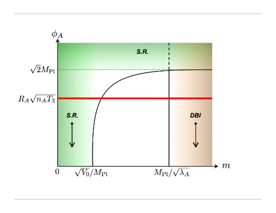
Figure 1: The inflation phase diagram for UV models. The shaded regions correspond to parameter space that can give rise to inflation. The darker the region is, the larger $e$-folds it can provide. “S.R.” stands for slow-roll inflation; “DBI” stands for DBI inflation. The arrows indicate the starting point and rolling direction of the inflaton. In brane inflation, inflatons have to stay below the horizontal solid line (at $\phi_{A}=R_{A}\sqrt{n_{A}T_{3}}$); the two vertical lines (at $m=\sqrt{V_{0}}/M_{\rm Pl}$ and $m=M_{\rm Pl}/\sqrt{\lambda_{A}}$) are widely separated. The curve stretching from $m=\sqrt{V_{0}}/M_{\rm Pl}$ to $\phi_{A}=\sqrt{2}M_{\rm Pl}$ corresponds to $\eta_{V}=\beta/3=1$. See text for discussion.

If the flatness of the potential $V(\phi)$ satisfies the slow-roll conditions, the branes can slowly roll non-relativistically and the kinetic term of the brane DBI action reduces to the minimal non-relativistic form. To indicate this condition in the phase diagram, we draw a curve of $\eta_{V}\equiv M_{\rm Pl}^{2}V^{\prime\prime}/V=1$ which is

$$\phi^{2}=2M_{\rm Pl}^{2}-\frac{2V_{0}}{m^{2}}~{},$$ (2.5)

where we neglected the Coulomb potential term for simplicity. Eq. (2.5) corresponds to the solid line stretching from the lower-left (at $m=\sqrt{V_{0}}/M_{\rm Pl}$) to upper-right (at $\phi=\sqrt{2}M_{\rm Pl}$) in Fig. 1. Inclusion of the Coulomb term will cause a slight deformation at the lower-left corner of this curve and will not affect our conclusion. The shaded region above and to the left of this curve has $\eta_{V}<1$, and corresponds to the slow-roll inflation phase; here the condition $\epsilon_{V}<1$ is always weaker. The lower-left shaded region is the small-field slow-roll region where the potential is dominated by the constant $V_{0}$. As $\phi$ increases toward the upper part of the shaded region, it corresponds to large-field slow-roll inflation where the potential is dominated by $m^{2}\phi^{2}$ term. Note that in this region $\phi$ is trans-Planckian, $\phi>\sqrt{2}M_{\rm Pl}$.

Outside of this slow-roll region, naively the inflaton will roll down the potential very fast and make inflation impossible. However because of the presence of the warped space, the velocity of the inflaton is bounded by the warped speed of light and therefore cannot be arbitrarily increased. Silverstein and Tong [33] show that, if

$$m\gg M_{\rm Pl}/\sqrt{\lambda_{A}}~{},$$ (2.6)

the inflaton enters another phase of inflation, namely DBI inflation, in which the full form the DBI kinetic term has to be taken into account. We indicate this condition by the solid vertical line (at $m=M_{\rm Pl}/\sqrt{\lambda_{A}}$) in Fig. 1 and the DBI inflation phase by the shaded region to the right.

There are two possible regions where these two phases merge onto each other: when the inflaton in the DBI phase starts from a Planckian value (the upper-right corner of Fig. 1), the inflation can go continuously from slow-roll to DBI; when $\sqrt{V_{0}}/M_{\rm Pl}\sim M_{\rm Pl}/\sqrt{\lambda_{A}}$ so the two vertical lines in Fig. 1 become very close to each other or even switch places, the inflaton around this border will trigger an inflationary phase that lies in-between the slow-roll and DBI regimes. These are the “intermediate regions” studied in Refs. [43, 26].

However, so far we have been discussing an effective field theory description where one is allowed to independently choose the throat charge $N_{A}$, fundamental string mass $m_{s}$ and the inflaton field range $\phi$. In a realistic string compactification like the generic multi-throat flux compactification in type IIB string theory [37], various throats are glued to a bulk. There are several fairly model-independent geometric conditions that should be imposed to be consistent with the brane inflation setup that we have in mind. In this type of compactification, the Planck mass is obtained by an integration throughout the compact space,

$$M_{\rm Pl}^{2}\sim g_{s}^{-2}m_{s}^{8}V_{6}~{},$$ (2.7)

where $V_{6}$ is the total volume of the compactification (after modding out the possible orbifold effect) and its dominant contribution comes from the bulk and the UV regions of throats. The throats are glued to the bulk and their sizes $R$ are restricted,

$$\frac{R_{A}^{6}}{a_{A}}\lesssim V_{6}~{}.$$ (2.8)

The volume of the throat is divided by $a_{A}$ in case of orbifolding. The inflaton brane separation is restricted by

$$\phi\lesssim R_{A}\sqrt{n_{A}T_{3}}~{},~{}~{}~{}{\rm or}~{}~{}~{}\phi\lesssim L\sqrt{n_{A}T_{3}}~{},$$ (2.9)

for $n_{A}$ branes moving in the throat or the bulk respectively. Here $L$ is the size of the bulk in a certain dimension. These conditions have been used in various contexts in brane inflation, to constrain slow-roll models in the bulk [21, 23], random walk eternal inflation [40], the UV DBI model through the non-Gaussianities [39, 41, 26, 38], and the tensor mode [41, 44, 45, 46]. For our phase diagram these imply

$$\frac{\sqrt{V_{0}}}{M_{\rm Pl}}\Bigg{/}\frac{M_{\rm Pl}}{\sqrt{\lambda_{A}}}\lesssim\frac{n_{A}h_{A}^{2}}{N_{A}/a_{A}}\ll 1~{},$$ (2.10)

and

$$\frac{R_{A}\sqrt{n_{A}T_{3}}}{M_{\rm Pl}}\lesssim\frac{\sqrt{n_{A}}}{\sqrt{N_{A}/a_{A}}}\ll 1~{}.$$ (2.11)

Thus the two vertical solid lines (at $m=\sqrt{V_{0}}/{M_{\rm Pl}}$ and $m=M_{\rm Pl}/\sqrt{\lambda_{A}}$ respectively) in Fig. 1 should be widely separated; the inflaton can only move below the horizontal solid line (at $\phi=R_{A}\sqrt{n_{A}T_{3}}$) which is well below $\phi=\sqrt{2}M_{\rm Pl}$. This excludes the large field models where $\phi\gtrsim M_{\rm Pl}$, and opens up a wide region in the middle of the parameter space where there is no inflation. This is also why random-walk eternal inflation in KKLMMT model within the throat is excluded in [40], the tensor mode in brane inflation is unobservable [41], and the “intermediate UV models” are ruled out in [26]. The earlier statement that the antibrane tension alone is not large enough to drive DBI inflation in UV models can be justified as well by estimating $H_{\rm anti}\Delta t\approx\sqrt{n_{A}T_{3}}R_{A}h_{A}/M_{\rm Pl}\ll 1$, where $H_{\rm anti}$ is the contribution from antibrane tension and $\Delta t\approx R_{A}h_{A}^{-1}$ is the time scale that the branes spend traveling down the throat.

Having considered this inflationary phase diagram, we can now restrict the parameter space by comparing it to observations. In the UV model, we saw from the above discussions that there is a clean separation of slow-roll and DBI inflationary phases after the geometric conditions (2.7)-(2.9) are applied. The slow-roll region is the KKLMMT model [23] and is compatible with the current observations [26, 47, 48]. In this model, the inflaton mass may be adjusted to fit the spectral index. The running of spectral index and non-Gaussianities are unobservable if the potential is featureless. The tensor mode is also unobservable. The DBI region is the STA model [33, 34]. It predicts large non-Gaussianities with the estimator

$$|f_{NL}^{\rm eq}|\approx 1.3\frac{p^{2}M_{\rm Pl}^{4}}{\phi^{4}}~{},$$ (2.12)

(where $p=m/(\sqrt{6}M_{\rm Pl}/\sqrt{\lambda_{A}})\gg 1$,) together with a possibly-observable tensor mode $r\approx 5/(p\sqrt{f_{NL}})$ [34]. From the constraints (2.9) and (2.11), one can see that, for one brane $n_{A}=1$, $|f_{NL}|\gtrsim p^{2}(N_{A}/a_{A})^{2}$ which cannot fit the observations [26, 39, 41]. One way to increase the field range is to increase the number of the inflaton branes. Here we emphasize another constraint coming from the relativistic probe brane backreactions discussed in [33, 53]. In order to treat the mobile inflaton branes as probes of the warped background, $N_{A}/a_{A}\gg n_{A}\gamma$ is required. Namely, the energy scale of the mobile branes cannot exceed the source of the warped background. On the other hand, combining (2.9), (2.11) and (2.12), we have $|f_{NL}|\gtrsim 1.3p^{2}N_{A}^{2}/(a_{A}^{2}n_{A}^{2})$. Using the relation $|f_{NL}|\approx 0.32\gamma^{2}$, these two requirements lead to $p\ll 0.5$, which is a contradiction. Note that this conclusion is independent of the value of $n_{A}$ and before any comparison with data is made. However we should note that this inconsistency appears when the STA model is embedded in the warped compactification of the GKP type, so it remains a viable field-theoretic model, and looking for other UV embeddings becomes an interesting question.

2.2 IR models

In the IR models, branes are started from the IR side of a throat (denoted as the B-throat) and roll toward the UV side under the moduli potential

$$V(\phi)=V_{0}-\frac{1}{2}m^{2}\phi^{2}~{}.$$ (2.13)

The origin of $\phi$ is at the tip of the throat (2.2), which can be realized for example if the tip of the throat is an orbifold fixed point. The Coulomb attraction from antibranes in other throats is neglected here unless $m^{2}/H^{2}$ is very small.

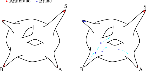
Figure 2: Multi-throat brane inflation scenario. In the first figure, antibranes are settled down in throats. In the second figure, in some throats antibranes annihilate fluxes and generate branes. For a throat with tachyonic brane moduli, branes fall out and settle down somewhere else, triggering either IR or UV models of brane inflation.

The IR model can arise in the following scenario [35] (illustrated in Fig. 2): At the beginning, antibranes are naturally attracted to and settle down at the end of various throats induced by fluxes. However they are semi-stable at most, and will eventually annihilate against some fluxes [51]. The end products are many branes. As mentioned, unlike antibranes, branes experience no potential if the extra dimensions are not compactly stabilized. But for realistic inflation models in string compactification, their moduli space is lifted. If the mass term is tachyonic as in (2.13) for a B-throat, these liberated branes will roll out. The inflationary energy $V_{0}$ is provided by longer-living antibranes in other throats (denoted as the A-throats) or in the bulk. Shorter A-throats give more dominant contributions to $V_{0}$. These antibranes eventually get annihilated by some of the inflaton branes. The annihilation products will naturally heat low mass-scale sectors in case of tunnelling reheating [52], such as branes residing in very long throats or in a large bulk.

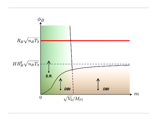
Figure 3: The inflation phase diagram for IR models. The notation used here is the same as in Fig. 1. The vertical line at $m=\sqrt{V_{0}}/M_{\rm Pl}$ corresponds to $|\eta_{V}|=\beta/3=1$. The unshaded region may support a certain amount of non-relativistic fast-roll inflation.

In the absence of the warped space, the $|\eta_{V}|\equiv M_{\rm Pl}^{2}|V^{\prime\prime}|/V=1$ line is

$$\phi^{2}=-2M_{\rm Pl}^{2}+\frac{2V_{0}}{m^{2}}~{},$$ (2.14)

which corresponds to the vertical line (at $m=\sqrt{V_{0}}/M_{\rm Pl}$) in Fig. 3. Slow-roll inflation occurs when $|\eta_{V}|<1$ which is the region to the left of this line.

In the presence of the warped space, DBI inflation can be triggered even if the slow-roll condition is not satisfied. Ref. [35, 36] show that, for $\beta\equiv m^{2}/H^{2}\sim|\eta_{V}|\gtrsim 1$, DBI inflation happens if

$$\phi<HR_{B}^{2}\sqrt{n_{B}T_{3}}~{}.$$ (2.15)

Here, an important difference from the STA model condition (2.6) is that, because the inflationary energy $V_{0}$ is provided by antibranes in other throats instead of the moduli potential itself, the shape of the potential that can achieve inflation becomes rather flexible. Of the special interest is the generic case $m^{2}\sim H^{2}$. Even for $\beta<1$ when slow-roll inflation is possible, the speed-limit provided by the warped space cannot be neglected if the inflatons are started from the region [36]

$$\phi<\beta HR_{B}^{2}\sqrt{n_{B}T_{3}}~{}.$$ (2.16)

This implies that the DBI and slow-roll phases can be smoothly connected by an intermediate region in this corner of the parameter space. Overall, the DBI inflation phase stays below the horizontal curve stretching from the origin to $\phi=HR_{B}^{2}\sqrt{n_{B}T_{3}}$ in Fig. 3. The DBI region always stays well below the maximum inflaton extension (the horizontal solid line at $\phi=R_{B}\sqrt{n_{B}T_{3}}$), since

$$\frac{HR_{B}^{2}\sqrt{n_{B}T_{3}}}{R_{B}\sqrt{n_{B}T_{3}}}=HR_{B}\lesssim\frac{\sqrt{n_{A}}h_{A}^{2}}{\sqrt{N_{B}/a_{B}}}\ll 1~{},$$ (2.17)

where

$$V_{0}=2n_{A}h_{A}^{4}T_{3}~{},$$ (2.18)

and (2.7) (2.8) are used, $n_{A}$ being the number of antibranes that get annihilated. We see that IR DBI inflation is completed in a very small region at the tip of the B-throat. Unlike the UV DBI phase, the condition (2.9) is automatically satisfied. This also justifies the small field expansion in (2.13).

We have treated the Hubble parameter $H$ as a constant. This can be verified using the geometric constraints (2.7) and (2.8), because in the IR model the potential drop $\Delta V$ during inflation, estimated very conservatively, satisfies

$$\frac{\Delta V}{V_{0}}\lesssim\frac{m^{2}R_{B}^{2}n_{B}T_{3}}{2V_{0}}\sim\frac{\beta n_{B}}{N_{B}/a_{B}}~{}.$$ (2.19)

As long as

$$\beta\ll N_{B}/(a_{B}n_{B})~{},$$ (2.20)

the inflationary energy is approximately a constant.

Therefore we see that in the IR models, inflation can occur for a large range of the mass parameter,

$$0<m^{2}/H^{2}\ll N_{B}~{},$$ (2.21)

around the generically expected magnitude $m\sim H$. The requirement is to start the inflatons from a small enough $\phi_{B}$. In terms of the flux compactification this is easy to achieve, because the minimum warp factor is given by the flux numbers $M$ and $K$ in an exponential form [37]

$$h_{\rm min}\sim\exp(-2\pi K/3Mg_{s})~{}.$$ (2.22)

We emphasize that non-trivial constraints come from various back-reactions that cut off the IR regions of a throat. These include the back-reaction from the 4-d inflationary background [36, 52] and the back-reaction from the relativistic inflaton branes [33, 53]. The former is generally (for $\beta\sim 1$) more important than or comparable to the latter depending on the number of inflaton branes. It is estimated [36, 52] to cut off the throat at $\phi\sim HR_{B}^{2}\sqrt{n_{B}T_{3}}/\sqrt{N_{B}}$. This determines the maximum number of $e$-folds achievable by the DBI inflationary phase, $N_{\rm tot}^{\rm DBI}\sim\sqrt{N_{B}}$. A more detailed understanding of this backreaction is important.

It is worth pointing out that, in terms of model building, the most important difference between the IR and UV DBI models is not whether branes are started from the IR or UV side of a warped space. It is the independence between the inflaton speed-limit and the inflationary energy, which allows a flexible shape of potential. We have seen that this naturally happens when branes are moving out of a throat, with inflationary energy provided by antibranes in other throats. Just in terms of field theory, even in the UV models, such an independence can be achieved by demanding the constant term $V_{0}$ in the potential (2.1) to be independent of the A-throat warp factor, for example by a hybrid of a different field around $\phi=0$ to suddenly end inflation. The question is then how to realize it naturally in string models.

Having considered the phase diagram, we would like to first restrict the parameter space by comparing the predictions of the model with observational data, and then make predictions for future observations. This will be the main focus for the rest of the paper. We close this subsection with a few comments on the setup of the model.

Firstly, as we demonstrated in Fig. 1, for UV models there is no inflation around $\eta_{V}\sim 1$ and a large parameter space beyond that. So for IR models, it is reasonable to consider the simplest case where, after branes come out of the B-throat, there is no significant amount of additional inflationary $e$-folds if they roll through the bulk or enter another A-throat to annihilate antibranes there. This simplest possibility represents a fairly generic class of models.

Secondly, more realistic throats such as the Klebanov-Strassler throat [54] have a scale-dependent charge. The characteristic scale $R$ decreases slowly towards the tip of the throat. Especially the geometry around the tip region will be significantly different from (2.2). For UV models such modifications can be important because the tip of the throat is the region around which the last 60 $e$-folds of inflation happens [55, 56]. For IR models, the situation is opposite. The last 60 $e$-folds of inflation happens away from the bottom of a throat because generally the total $e$-folds is more than 60. Furthermore the relevant field range is very small. Therefore, under these conditions (which will be made more precise in Sec. 3.1), we can ignore both the deformation of the throat geometry and the running of the throat charge, and approximate the metric as (2.2) with the constant $\lambda$ (or $R$) being the effective value at the relevant $\phi$ (or $r$).

Thirdly, as we have mentioned, the realistic IR case almost always involves multiple inflaton branes. It is interesting to see whether the non-Abelian action plays an important role [57]. In our scenario, after the mobile branes are created in the IR end of the throat, they all have approximately the same radial coordinates and roll in the radial direction. In the angular directions, we either imagine that they are randomly distributed, in which case their average separation is $h_{B}R_{B}/n_{B}^{1/5}$ (the power of $1/5$ is due to the five-sphere) which is much larger than the local red-shifted string length along the extra dimensions, $h_{B}m_{s}^{-1}$; or we imagine that they stick together and roll with a fixed angular coordinate, which is different from them forming a higher dimensional brane and expanding around the center. In both cases, we expect the leading effects of a large number of branes on density perturbations to be well represented by the Abelian action. As in Ref. [36, 39], we will use this approximation in this paper.

Lastly, there is a trivial slow-roll region in IR models if we tune $\beta$ to be near ${\cal O}(0.01)$. We skip this parameter space in this paper and start from $\beta\gtrsim{\cal O}(0.1)$.

2.3 Open questions

We list two open questions that are relevant to our parameterization:

$\bullet$ Construction of potentials: Different parameter regions in the phase diagrams have different requirements on the inflaton mass. As mentioned, the generic magnitude of the inflaton mass is expected to be of order $H$, but the actual value can be environmental. For the slow-roll phases in both UV and IR models, such a mass term has to be tuned to percent level of the generic value; for the IR DBI model, although the magnitude of the inflaton mass can be of the generic order, it has to be tachyonic, or more generally the potential has to be repulsive for branes. For example, the conformal coupling will give a positive mass-squared $2H^{2}$ (through the canonical inflaton dependence in the Kähler potential). It is possible that such a contribution gets cancelled by others from the superpotential or Kähler potential, to order $0.01H^{2}$ for slow-roll models. For IR DBI models, it has to be cancelled to a negative value, although inflation is insensitive to the magnitude. In addition it is easy to see that, for IR DBI inflation to happen, the shape of the repulsive potential can be much more general than the quadratic form [58]. For the UV DBI model, the requirement seems to be more restrictive. The typical potential is expected to vary over $\Delta\phi\lesssim m_{s}\ll M_{\rm Pl}$, so to have a quadratic form over Planckian size $\Delta\phi$ needs to be functionally fine-tuned. In addition, using the geometric conditions (2.7) and (2.8), the requirement (2.6) implies

$$m\gg M_{\rm Pl}/\sqrt{\lambda_{A}}>\frac{N_{A}^{1/4}}{g_{s}^{1/4}a_{A}^{1/2}n_{A}^{1/2}}m_{s}~{}.$$ (2.23)

In string constructions, the mass parameters typically arise at most of order of the string scale $m_{s}$, with possible suppressions from factors of the Planck mass $m_{s}/M_{\rm Pl}$ and warp factors. So $a_{A}\gg\sqrt{N_{A}/g_{s}}/n_{A}$ is necessary, where $a_{A}$ is defined before (2.4) and is due to orbifolding. The construction of all these potentials is an issue under active investigation [59, 60, 61, 62, 63].

$\bullet$ Background D3-charges: As we have seen, to get enough $e$-folds in the DBI model, $N_{B}\sim 10^{4}$ is enough. But as we will see later, there are interesting parameter spaces in DBI inflation which require very large D3-charges for the A or B-throat to fit the magnitude of the density perturbations. This charge can be as large as of order ${\cal O}(10^{14})$ [34]. In IR models, branes are always generated in a large number after the flux-antibrane annihilation, and this reduces $N_{B}$ to ${\cal O}(10^{9})$ [36]. In a GKP-type flux compactification, such a charge should be cancelled by the induced negative D3-charge of the wrapped D7-branes. This negative charge is given by the Euler number of the corresponding fourfold in F-theory. The explicit examples give no more than ${\cal O}(10^{5})$ [64]. So far it is not clear which of the following possibilities is true: in terms of the density perturbations, DBI inflation is extremely fine-tuned or even not viable; a modified construction, e.g. multiple-dimensional orbifolding (a large $a_{A}$), can be engineered; a more complete understanding of the flux compactification can give such numbers; or subtleties are involved in the reheating.

The approach in this paper to both issues above is phenomenological. By parameterizing and comparing them to experimental data, we can hopefully learn something useful about string theory from a bottom-up approach.

3 IR DBI model

In this section, we summarize the main results and predictions of the IR model, carrying out numerical calculations whenever is necessary. In the next section, we compare them to observational data, constrain microscopic parameters and make predictions.

3.1 Attractor solutions

In regions where various back-reactions to the warped background are negligible and the Hubble energy stays below the red-shifted string scale, the low-energy dynamics of the inflaton branes is described by the DBI-CS action

$$S=\frac{M_{\rm Pl}^{2}}{2}\int d^{4}x\sqrt{-g}R-\int d^{4}x\sqrt{-g}\left(\frac{\phi^{4}}{\lambda_{B}}\sqrt{1+\frac{\lambda_{B}}{\phi^{4}}g^{\mu\nu}\partial_{\mu}\phi\partial_{\nu}\phi}-\frac{\phi^{4}}{\lambda_{B}}+V(\phi)\right)~{},$$ (3.1)

where $V(\phi)$ is given by (2.13). The branes start from the tip of the throat and end at the UV end of the throat $\phi_{\rm end}=R_{B}\sqrt{n_{B}T_{3}}=\sqrt{\lambda_{B}}/R_{B}$. After that some of them quickly find antibranes and annihilate, diminishing the cosmological constant $V_{0}$.

The dynamics of the inflaton can be approximately described by two attractor solutions. The first is that of the IR DBI inflation. This is the phase where the effect of the speed-limit is important. The inflaton is traveling near the warped speed of light, and the attractor solution is

$$\phi=-\frac{\sqrt{\lambda_{B}}}{t}+\frac{9\sqrt{\lambda_{B}}}{2\beta^{2}H^{2}t^{3}}+\cdots~{},$$ (3.2)

where $t$ is chosen to run from $-\infty$ for convenience. Recall that for $0<\beta\ll N_{B}/(a_{B}n_{B})$, $H$ is approximately a constant. This phase ends around $\phi\sim H\sqrt{\lambda_{B}}$ ($t\sim-H^{-1}$) for $\beta\gtrsim 1$ and $\phi\sim\beta H\sqrt{\lambda_{B}}$ ($t\sim-\beta^{-1}H^{-1}$) for $\beta<1$. The inflationary $e$-folds as the function of $\phi$ can be estimated as

$$N_{e}^{\rm DBI}\approx\frac{H\sqrt{\lambda_{B}}}{\phi}-\beta^{-1}~{}.$$ (3.3)

Here we have incorporated both the case $\beta<1$ and $\beta\gtrsim 1$ by adding the term $\beta^{-1}$; this correction is negligible for $\beta\gtrsim 1$, and the validity of (3.2) requires $N_{e}^{\rm DBI}\gg\beta^{-1}$.

The second attractor solution describes the nonrelativistic rolling where the inflaton velocity stays far below the speed-limit. In this limit the equation of motion

$$\ddot{\phi}+3H\dot{\phi}+\partial_{\phi}V(\phi)=0$$ (3.4)

has the following attractor solution

$$\phi=\phi_{0}e^{\alpha\beta H(t-t_{0})/3}~{},~{}~{}~{}~{}~{}\alpha=\frac{-9+\sqrt{81+36\beta}}{2\beta}~{}.$$ (3.5)

The consistency condition that the inflaton velocity is non-relativistic $\dot{\phi}\ll\phi^{2}/\sqrt{\lambda_{B}}$ requires that $\phi\gg\alpha\beta H\sqrt{\lambda_{B}}/3$. This phase is smoothly connected to the previous DBI phase. The total number of inflationary $e$-folds provided by this period is given by

$$N_{\rm tot}^{\rm NR}\approx\frac{3}{\alpha\beta}\ln\phi\Bigg{|}_{\alpha\beta H\sqrt{\lambda_{B}}/3}^{\sqrt{\lambda_{B}}/R_{B}}\approx\frac{3}{\alpha\beta}|\ln HR_{B}|~{}.$$ (3.6)

We emphasize that this nonrelativistic rolling region is slow-roll only if $\beta\ll 1$, while the above formulae are valid even if this condition is not satisfied. For example in Fig. 3 at around $\beta\sim 1$ ($m\sim\sqrt{V_{0}}/M_{\rm Pl}$), after the DBI phase it takes time for branes to go through the lightly-shaded region till it reaches the end of the throat. This is because the branes are originally very close to the top of the potential. It provides a certain amount of $e$-folds typically not corresponding to the scale of the CMB. These additional non-relativistic non-slow-roll inflationary $e$-folds is also interesting to us, because it affects the relevant $e$-folds in the DBI phase,

$$N_{e}=N_{e}^{\rm DBI}+N_{\rm tot}^{\rm NR}~{},$$ (3.7)

and hence predictions for observations.

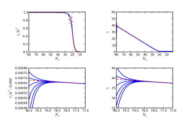
Figure 4: Attractor solutions and numerical results. The dashed lines are the analytical attractor solutions. The solid lines are numerical solutions with different initial velocities. The upper-left panel shows the evolution of the ratio of the inflaton-velocity $\dot{r}$ to the warped-speed-of-light $h^{2}$. The two dashed lines are DBI and non-relativistic rolling, respectively. The upper-right panel shows the evolution of the Lorentz factor $\gamma$. The lower panels are the blow-ups of the upper panels. The parameters are $\beta=2$, $N_{B}=10^{9}$, $n_{B}=10^{5}$, $m_{s}g_{s}^{-1/4}=10^{-6}M_{\rm Pl}$, $n_{A}h_{A}^{4}=1$. In the simulation, branes are started at $h_{B}=2.9\times 10^{-7}$.

In Fig. 4 we demonstrate numerical results and show that the two attractor solutions (3.2) and (3.5) give good analytical approximations for the inflaton dynamics. Any initial angular motions will also be damped out due to the Hubble friction, because the inflaton potential considered here has only radial dependence.

Klebanov-Strassler throat

In this paper, we use the $AdS_{5}$ geometry with a length scale $R$ to represent the warped space. The details of the geometry can be different for more realistic cases. We expect our example to capture the main properties of the model, and to be a good approximation for a certain generic parameter space. Let us consider, for example, the KS throat,

$$h(r)^{-4} = \frac{27\pi g_{s}\alpha^{\prime 2}}{4r^{4}}\left[N_{\rm tot}+\frac{3g_{s}M^{2}}{2\pi}\left(\ln\frac{r}{r_{max}}+\frac{1}{4}\right)\right]$$ (3.8)

$$\equiv \frac{R_{l}^{4}}{r^{4}}~{},$$

where we have defined a running $R_{l}$,

$$R_{l}^{4}=\frac{27\pi}{4}g_{s}\alpha^{\prime 2}N_{\rm eff}~{},$$ (3.9)

with $N_{\rm eff}\equiv MK_{\rm eff}=M(K_{\rm tot}-l)$ for

$$r=r_{max}\exp(-2l\pi/3g_{s}M)~{}.$$ (3.10)

So instead of the parameter $N_{B}$, here we have the parameter $M$. The effective $N_{\rm eff}$ and $K_{\rm eff}$ are now functions of $r$ or $l$. From (3.10) we can estimate that, during IR DBI inflation, $\Delta l\approx g_{s}M$. Therefore as long as

$$K_{\rm eff}\gg g_{s}M~{},$$ (3.11)

we can neglect the running of $N_{\rm eff}$. The $N_{B}$ in our analyses thus represents the $N_{\rm eff}$ in a small region of $r$ relevant for IR DBI inflation. The condition (3.11) is most easily satisfied by having a small $g_{s}$. In addition, since the WMAP window is only a few $e$-folds, which corresponds to $\Delta l\approx 3g_{s}M/N_{e}^{\rm DBI}$, we only need $K_{\rm eff}>g_{s}M$ to approximate $N_{\rm eff}$ as a constant in this window. In this case, the running of $N_{\rm eff}$ only slightly affects the total DBI $e$-folds, and hence the relation in (3.7). Another difference between the KS throat and the geometry we use is that, in the latter, the UV edge of the warped space is cut off and glued to the bulk at $R$, while in the former it is given by an independent parameter $r_{max}$. This does not cause too much difference in the analyses, since the non-relativistic fast-roll inflation mostly happens near the top of the potential; hence $N^{\rm NR}_{\rm tot}$ is insensitive to the cutoff in generic cases.

3.2 Power spectrum

We first look at the density perturbations in the DBI phase. Its amplitude is given by the usual formula

$$P_{k}=H^{2}\delta t^{2}~{},$$ (3.12)

where $\delta t$ is the position-dependent time delay caused by the frozen quantum fluctuations of the inflaton, $\delta\phi=H/2\pi$. In this phase we approximate the inflaton zero-mode velocity as the speed of light, $\dot{\phi}=\phi^{2}/\sqrt{\lambda_{B}}$. So we have

$$P_{k}=\frac{H^{4}}{4\pi^{2}\dot{\phi}^{2}}\approx\frac{(N_{e}^{\rm DBI})^{4}}{4\pi^{2}\lambda_{B}}~{}.$$ (3.13)

If this is responsible for $P_{k}\approx 23\times 10^{-10}$, we need $\lambda_{B}\sim 10^{13}$. Since the number of branes created after the flux-antibrane annihilation can be as large as ${\cal O}(\sqrt{N_{B}})$, this requires $N_{B}\gtrsim 10^{9}$. The formula (3.13) can be derived rigorously using the formalism of Garriga and Mukhanov [65], where we can see that the main difference from the slow-roll case is the development of the sound speed $c_{s}$ on the world-volume of the inflaton branes. This shrinks the Hubble horizon by a factor of $c_{s}$. The underlying physics can be most easily understood in the view of an instantaneous co-moving observer with the brane [35, 36]. For this observer the Hubble expansion rate is increased by the Lorentz factor

$$\gamma=1/c_{s}=1/\sqrt{1-\lambda_{B}\dot{\phi}^{2}/\phi^{4}}\approx{\beta N_{e}^{\rm DBI}\over 3}$$ (3.14)

due to the relativistic time dilation. In the last step of (3.14), we have used the IR model solution (3.2) and (3.3). This Hubble parameter leads to a horizon of size $c_{s}H^{-1}$, which lies orthogonal to the brane velocity and hence appears the same to the lab observer (i.e. the observer that does not move with the branes).

In this model it is very important to realize the validity condition for the field theory analyses of density perturbations, and make estimates for the density perturbations when the field theory analyses break down [35, 36, 39]. There are the following several interesting regions as we extend the inflaton back in time towards the IR side of the warped space.

Firstly, open strings on the inflaton brane will be created when the Hubble energy density $\gamma^{4}H^{4}$ for the moving observer becomes larger than the red-shifted brane tension $h_{B}^{4}T_{3}=\phi^{4}/n_{B}\lambda_{B}$. Using (3.3) and (3.14), this happens at the critical $e$-fold

$$N_{c}\sim\frac{\lambda_{B}^{1/8}}{\beta^{1/2}n_{B}^{1/8}}\sim\frac{N_{B}^{1/8}}{\beta^{1/2}}~{}.$$ (3.15)

Another observation that also indicates that we cannot naively extend the field-theoretic results too far down the IR side of the throat, is to look at the region $N_{e}>N_{c}$, where the brane fluctuations in the transverse directions become superluminal. This is impossible. The reason that such a superluminal speed even occurs under the DBI action can be understood as follows. When we calculate the primordial fluctuations, in the first step, the source of such fluctuations is the uncertainty principle, which a priori does not necessarily respect the speed-limit if we only consider the scalar field. In the next step, the later evolution of such fluctuations is governed by the DBI action and always follows the causality constraint. The superluminal fluctuation speeds to which we just referred come from the first step, if we naively extend the field theoretic calculation to the regions beyond (3.15).

Secondly, closed strings will be created when the Hubble energy $H^{4}$ for the lab observer becomes larger than the red-shifted brane tension. This happens at

$$N_{e}\sim\lambda_{B}^{1/4}/n_{B}^{1/4}~{}.$$ (3.16)

Finally, when the closed string density created by the Hubble expansion overwhelms the source (fluxes or branes) for the warped geometry, the warped space gets cut off. As mentioned, this back-reaction determines the maximum number of inflationary $e$-folds in the DBI phase,

$$N_{\rm tot}^{\rm DBI}\sim{\lambda_{B}^{1/2}}/{n_{B}^{1/2}}~{}.$$ (3.17)

It is important to note that the zero-mode dynamics of the inflaton are still valid as long as $N_{e}<N^{\rm DBI}_{\rm tot}$, since it only relies on the existence of the speed-limit and therefore on the condition (3.17) at which the warped space gets cut off. In addition, the strings and graviton KK-modes are only created in the tip of the throat and have energy density ${\cal O}(H^{4})$. It does not backreact significantly on the Hubble expansion. However, the field-theoretic calculation of the density perturbation is no longer valid if $N_{e}\gtrsim N_{c}$, since not only scalar fields but also open strings will be created.

While a rigorous treatment is currently unavailable, there are a couple of ways to estimate the density perturbations in this situation [36, 39]. (We shall make the estimates more quantitative in Appendix A.) We can estimate the part of energy that goes into scalar fluctuations to be saturated when the Hubble temperature reaches the brane tension $\phi^{4}/n_{B}\lambda_{B}$ at (3.15). Further relative increase of the Hubble energy excites strings and branes. The stringy excitations will be diluted by the exponential spatial expansion after the Hubble energy drops below the brane tension as branes move to the UV side, in the same way that the inflation dilutes relic densities. Only the scalar fluctuations are frozen and later translated into the position-dependent time-delay for the reheating. For the moving observer, the scalar field energy density is $(\delta\phi)_{\rm mov}^{2}\gamma^{2}H^{2}\sim\phi^{4}/n_{B}\lambda_{B}$ and for the lab observer $\delta\phi=\delta\phi_{\rm mov}/\gamma$. This estimate leads to $\delta\phi=\sqrt{\lambda_{B}}H/\sqrt{n_{B}}(N_{e}^{\rm DBI})^{2}\gamma^{2}$. So for $N_{e}>N_{c}$, we estimate

$$P_{k}=H^{2}\frac{\delta\phi^{2}}{\dot{\phi}^{2}}\sim\frac{324\pi^{2}}{n_{B}\beta^{4}(N_{e}^{\rm DBI})^{4}}~{}.$$ (3.18)

This is also the result that we will get by looking at the transverse fluctuation speed of each brane. The field-theoretic analyses lead to the fluctuation speed (for the moving observer), $\dot{r}_{\rm mov}=\delta r/\delta t\approx{\gamma H\over\sqrt{T_{3}}}/(\gamma H)^{-1}$, which is the fluctuation amplitude divided by a Hubble time. This velocity reaches the warped speed of light precisely around (3.15). Above the phase transition, we assume the fluctuation speed saturates the warped speed of light $h^{2}$, so $\delta r_{\rm mov}\approx h^{2}(\gamma H)^{-1}$. The position-dependent time-delay is then

$$\delta t_{\rm lab}\approx\frac{\delta r_{\rm mov}/\dot{r}_{0}}{\gamma\sqrt{n_{B}}}\approx\gamma^{-2}H^{-1}/\sqrt{n_{B}}~{},$$ (3.19)

where $\dot{r}_{0}=h_{B}^{2}$ is the zero-mode brane speed, and the factor $1/\sqrt{n_{B}}$ is due to the reduction of the root-mean-square of the fluctuations by the superposition of $n_{B}$ independent branes. Eq. (3.19) reproduces (3.18).

3.3 Regional large running of spectral index and phase transition

From the last subsection, the spectral index is

$$n_{s}-1=\frac{d\ln P_{k}}{d\ln k}\approx-\frac{4}{N_{e}^{\rm DBI}}$$ (3.20)

for $N_{e}^{\rm DBI}<N_{c}$, and

$$n_{s}-1\sim\frac{4}{N_{e}^{\rm DBI}}$$ (3.21)

for $N_{e}^{\rm DBI}>N_{c}$.

The most interesting information from (3.15) is its smallness due to the power $1/8$. For $\lambda_{B}\sim 10^{13}$, $\lambda_{B}^{1/8}\sim{\cal O}(100)$, which already makes $N_{c}$ interestingly small. Considering the more realistic multi-brane case $n_{B}\lesssim\sqrt{N_{B}}$ leads to even smaller $N_{c}$ of order ${\cal O}(10)$. So such an interesting phase transition may well have occurred within our CMB scale. Another interesting property is the fact that Eq. (3.15) is independent of the inflationary energy scale and the local warp factor of the inflaton branes, so it will be a rather generic prediction of the IR DBI models.

It is very important how sharp this transition is in terms of $e$-folds. In Appendix A, we give an estimate of the transition width based on the following approach. For the familiar case of field-theoretic density perturbations, the super-horizon perturbations can be understood as being generated by the random walk of the transverse brane fluctuations within a Hubble time before the modes exit the horizon. Such a random walk velocity is given by the Hubble energy, and is non-relativistic. As we have discussed, during or above the stringy phase transition, the main difference is that the Hubble energy is comparable to or exceeds the rest mass of the brane in a Hubble-size patch. As a consequence the brane fluctuation speed becomes relativistic. We therefore use the same physical picture underlying the familiar theory, but generalize it relativistically to estimate the behavior of the density perturbations across the phase transition. The result is given in (A.4).

It is worth noting that this scenario has marked differences to several other cases commonly discussed in the literature. Firstly, this model has a scale-varying running of $n_{s}$, in contrast to the commonly investigated empirical ansatz, where the running of $n_{s}$ is assumed to be constant. Here the large running of $n_{s}$ is only regional, principally when $N_{e}^{\rm DBI}\lesssim N_{c}$. Secondly, this scenario can generate large running, in contrast to most slow-roll scenarios. A standard slow-roll potential predicts very small running of $n_{s}$. A transient, large $dn_{s}/d\ln k$ can be caused by some “mild features” in the potential. For example, for small field slow-roll inflation, to generate a large transition for $n_{s}$ from blue to red, the mild feature should be a potential shape changing from concave to convex. We study this case in Appendix B. Since the spectral index is still close to one, the slow-roll parameters for this case should still be at least of order $0.1$. So such a case predicts unobservable non-Gaussianities. Lastly, non-standard choice of vacua may also cause observable running of spectral index. As we will discuss in Appendix C, such a running will be oscillatory in the WMAP window and phenomenologically distinguishable from the phase transition in IR DBI inflation.

3.4 Large non-Gaussianity and small tensor mode

The three-point function of the scalar perturbation for general single field inflation models, where the Lagrangian is an arbitrary function of $X=-\frac{1}{2}g^{\mu\nu}\partial_{\mu}\phi\partial_{\nu}\phi$ and $\phi$, is derived in Ref. [66]. In the absence of any sharp features [30], large non-Gaussianities can arise if the sound speed $c_{s}\ll 1$ or another quantity $\lambda/\Sigma\gg 1$ (related to the third derivative of the Lagrangian with respect to $X$). This non-Gaussianity is a function of three momenta, which are conveniently referred to as the shape of the non-Gaussianity [67] and the running of the non-Gaussianity [39]. The former describes its dependence on the shape of the momenta triangle, and the latter the overall size of the triangle. In the absence of sharp features, the running is relatively weak, and the shape has two categories: (1) the “local shape” in which the non-Gaussianity blows up in the squeezed-limit (where one of the momenta goes to zero) and takes a minimum value in the equilateral-limit (where all three momenta are equal); (2) the “equilateral shape” in which the non-Gaussianity vanishes in the squeezed-limit and reaches maximum value in the equilateral limit. The primordial non-Gaussianity is considered to be possibly observable if its estimator $f_{NL}$ is $|f^{\rm loc}_{NL}|>2$ or $|f^{\rm eq}_{NL}|>10$ [69, 70], where the superscript “loc” refers to the local shape and “eq” the equilateral shape.

For DBI inflation, the result becomes [34]

$$f_{NL}^{\rm eq}\approx-0.32c_{s}^{-2}~{}.$$ (3.22)

For IR DBI inflation, using the relation (3.14), we have [39]

$$f_{NL}^{\rm eq}\approx-0.036\beta^{2}(N_{e}^{\rm DBI})^{2}~{}.$$ (3.23)

The current observational bound is $-256<f_{NL}^{\rm eq}<332$ [68]. Comparing (2.12) and (3.23), we see that the requirements of the non-Gaussianity bound on the fundamental parameters are quite different. Furthermore the running of non-Gaussianities for these two cases are opposite, as dictated by the background geometry scanned through by the rolling inflatons.

However, we emphasize that the above results are derived in the regime where the primordial fluctuations are field-theoretic. Therefore the results can be different when the stringy phase transition happens. As we will see, data analysis suggests that the critical scale $k_{c}$ for that transition lies somewhere near the largest scales. For those smaller scales, it seems reasonable to assume that the magnitude of Eq. (3.23) should be smoothly modified by the stringy corrections. So in this paper, we will use this field-theoretic approximation (3.23) and the bound $|f_{NL}^{\rm eq}|<256$.

For DBI inflation, the scalar and tensor perturbations can be written as follows,

$$P_{k}=\frac{fV^{2}}{36\pi^{2}M_{\rm Pl}^{4}}~{},~{}~{}~{}~{}~{}~{}P_{h}=\frac{2V}{3\pi^{2}M_{\rm Pl}^{4}}~{},$$ (3.24)

where $f(\phi)$ is the background geometry and for our case $f=\lambda_{B}/\phi^{4}$. So the tensor to scalar ratio is

$$r_{TS}\equiv\frac{P_{h}}{P_{k}}=\frac{24\phi^{4}}{\lambda_{B}V}~{}.$$ (3.25)

Because $V$ is almost a constant in this model, the fact that the scalar and tensor modes have different horizon sizes during inflation makes no difference to (3.25). From Sec. 3.1, we see that, at the scale of $N_{e}^{\rm DBI}$, $\phi\approx HR_{B}^{2}\sqrt{n_{B}T_{3}}/N_{e}^{\rm DBI}$. So we get

$$r_{TS} \approx \frac{8}{{N_{e}^{\rm DBI}}^{4}}(HR_{B})^{2}\frac{n_{B}R_{B}^{2}T_{3}}{M_{\rm Pl}^{2}}$$ (3.26)

$$\lesssim \frac{1}{{N_{e}^{\rm DBI}}^{4}}\frac{n_{A}h_{A}^{4}}{N_{B}/a_{B}}\frac{n_{B}}{N_{B}/a_{B}}~{}.$$

This is of course consistent with the Lyth bound [73, 41, 44], since the r.h.s. of (3.26) is just the square of $\Delta\phi/\Delta N_{e}$ in Planck units divided by $(N_{e}^{\rm DBI})^{2}$, as we can see from (2.11), (2.17) and (3.3). To ignore the probe brane back-reactions we need $\gamma n_{B}\ll N_{B}/a_{B}$. So

$$r_{TS}\ll 1/({N_{e}^{\rm DBI}}^{4}\gamma^{2})<10^{-6}~{},$$ (3.27)

which is unobservably small. Therefore in our data analyses, we always set $r_{TS}=0$.

3.5 Constraining microscopic parameters

In this subsection we identify the set of microscopic parameters of the model, and list self-consistency constraints and the observables. As discussed in Appendix A, we can estimate the power spectrum at all scales across the transition region by the following formula,

$$P_{k}=\frac{4\pi^{2}v^{2}T_{3}}{\gamma^{4}\dot{\phi}^{2}}~{},$$ (3.28)

where

$$v^{2}T_{3}=h_{B}^{4}T_{3}\left[1-\left(1+\vphantom{\Biggl{(}}\displaystyle{\frac{\gamma^{4}H^{4}}{32\pi^{4}h_{B}^{4}T_{3}}}\right)^{-2}\right]=\vphantom{\Biggl{(}}\displaystyle{\frac{\phi^{4}}{n_{B}\lambda_{B}}\left[1-\left(1+\vphantom{\Biggl{(}}\displaystyle{\frac{n_{B}\lambda_{B}\gamma^{4}H^{4}}{32\pi^{4}\phi^{4}}}\right)^{-2}\right]}~{}.$$ (3.29)

These equations relate the fundamental parameters to the observations. We will always choose initial position and velocity of branes so that all the observable scales are within the attractor solution, namely the total $e$-folds is larger than the minimum requirement. So these initial conditions will not enter the observables. The parameters $V_{0}$ and $\beta\equiv m^{2}/H_{0}^{2}$ determine the scale and shape of the relevant part of the potential, $\lambda_{B}/n_{B}$ characterizes the background geometry, and $R_{B}$ tells us where to end the inflation (i.e. at $\phi_{\rm end}=\sqrt{32\pi^{2}/27}\sqrt{\lambda_{B}}/R_{B}$). So these four parameters determine the zero-mode evolution of the spacetime background and the inflaton dynamics in terms of the number of inflationary $e$-folds to the end of the inflation. In particular this determines the evolution of $\gamma$, $\phi/\sqrt{n_{B}}$ and $H$ in (3.28) and (3.29). Note that we can write the factor $h_{B}^{4}T_{3}$ in (3.29) in terms of $\phi/\sqrt{n_{B}}$ and $\lambda_{B}/n_{B}=2\pi^{2}N_{B}$, $h_{B}^{4}T_{3}=(\phi/\sqrt{n_{B}})^{4}/(\lambda_{B}/n_{B})$, so this is also determined. Because the factor $\dot{\phi}^{2}$ appears in the denominator of (3.28), the parameter $n_{B}$ affects the overall scale of $P_{k}$, but does not affect the spectral index once $\lambda_{B}/n_{B}$ is fixed. In conclusion, we have five parameters $\{\lambda_{B},n_{B},R_{B},V_{0},\beta\}$. Using (2.4) and (2.18), these parameters are equivalent to five even more fundamental microscopic parameters $\{N_{B},n_{B},m_{s}g_{s}^{-1/4},n_{A}h_{A}^{4},\beta\}$.

We have the following observables:

1. The amplitude of the power spectrum $P_{k}\approx 23\times 10^{-10}$. Through (3.13) and (3.18) this roughly determines the order of magnitude of the parameters $\lambda_{B}$ or $n_{B}\beta^{4}$ depending on whether the pivot point $N_{e}$ is smaller or larger than $N_{c}$.

2. The scale-dependence of $P_{k}$. This determines the spectral index and its running. Since the spectral index of this model has a regional large running, the data will constrain at which scale ($k_{c}$) such a running happens and which DBI $e$-fold ($N_{c}$) it corresponds to. These are then transferred into some delicate relations with the microscopic parameters, e.g. (A.7) and (3.7).

3. Non-Gaussianity constraint $\gamma<28$, will mainly constrain $\beta$ (with some weak dependence on $N_{e}^{\rm DBI}$).

4. We have the following several consistency relations. First, a scale $k$ is related to the corresponding $N_{e}$ by

   $$N_{e}=65-\ln\frac{k}{0.002\ {\rm Mpc}^{-1}}+\ln\frac{H_{0}/\hat{c}_{s}}{T_{\rm reheat}}~{},$$ (3.30)

   where the reheating is assumed to be efficient so that $T_{\rm reheat}=V_{0}^{1/4}$, and $\hat{c}_{s}$ is the sound speed when the mode $k=0.002\ {\rm Mpc}^{-1}$ crossed the sound horizon.

   Second, according to the multi-throat brane inflationary scenario, the maximum number of the inflaton branes is bounded by the flux number $M$. Since $N_{B}=a_{B}KM$ and we want to keep the minimum warp factor (2.22) small, we require

   $$n_{B}\lesssim\sqrt{N_{B}/(a_{B}g_{s})}~{}.$$ (3.31)

   Third, the geometric constraints (2.7) and (2.8) give an upper bound on $m_{s}g_{s}^{-1/4}$,

   $$\frac{m_{s}}{g_{s}^{1/4}}\lesssim 2^{3/2}\pi^{11/4}a_{B}^{1/2}\frac{M_{\rm Pl}}{N_{B}^{3/4}}~{},$$ (3.32)

   where the approximate numerical factors come from the toroidal compactification, $M_{\rm Pl}^{2}=\frac{2}{(2\pi)^{7}}g_{s}^{-2}m_{s}^{8}V_{6}$, which may change for more realistic setups.

   Fourth, the warp factor $h_{A}\leq 1$ and $n_{A}=n_{B}$, (this is not a coincidence, see footnote 7), so

   $$n_{A}h_{A}^{4}\leq n_{B}~{}.$$ (3.33)

   Lastly, the inflationary scale and the string scale are both bounded below by TeV,

   $$n_{A}h_{A}^{4}T_{3}\geq{\rm TeV}^{4}~{},$$ (3.34)

   $$m_{s}g_{s}^{-1/4}\geq{\rm TeV}~{}.$$ (3.35)

   (These two bounds turn out to be very weak. Much stronger ones will arise from the data analyses.)

   Note that, there are two other independent parameters $g_{s}$ and $a_{B}$ that only appear in the bounds (3.31) and (3.32). For simplicity we do not promote them into free parameters in data analyses. We set $g_{s}=0.1$ and $a_{B}=1$ in these bounds. Reducing $g_{s}$ and/or increasing $a_{B}$ may loosen these bounds and allow some microscopic parameters to take wider ranges. But this should not change the model predictions qualitatively.

4 Markov Chain Monte Carlo data analysis

4.1 Methodology

In order to obtain multi-dimensional parameter constraints from cosmological data, a Markov Chain Monte Carlo (MCMC) approach [74, 75, 76, 77, 78, 79, 80] is employed to sample the likelihood surface efficiently. The MCMC is used to simulate observations from the posterior distribution $P(\alpha|x)$, for a set of parameters $\{\alpha\}$ given an event $\{x\}$ (which, for us, is the total set of observational data), using Bayes’ Theorem

$$P(\alpha|x)=\frac{P(x|\alpha)P(\alpha)}{\int P(x|\alpha)P(\alpha)d\alpha}$$ (4.36)

where $P(x|\alpha)$ is the likelihood of the event $x$ given the model parameters $\alpha$, and $P(\alpha)$ is the prior probability distribution of obtaining a model parameter value $\alpha$. The MCMC generates random draws from the posterior distribution that are a “fair” sample of the likelihood surface, and from this sample, we can estimate all the quantities of interest about the posterior distribution (mean, variance, confidence levels).

In most cosmological analyses, flat priors, $P(\alpha)$=constant, are assumed on a set of empirical parameters such as the spectral index and its running, $n_{s}$, $dn_{s}/d\ln k$, and the normalization $A_{s}$, of the primordial scalar power spectrum, or its logarithm $\ln A_{s}$ (for example [28, 81, 2, 82, 26]). It is by no means true, however, that such constant priors should naturally arise in a fundamental theory. The effect of priors on constraints on slow-roll inflation was recently discussed in [83]; here we discuss their role in IR DBI inflationary scenarios.

Unlike parameters used in an empirical ansatz, the relationships between the fundamental microscopic parameters and observables are highly nonlinear and far from transparent. This can make it problematic for the MCMC to efficiently explore the likelihood surface, potentially leading to the presence of non-Gaussian posterior distributions: for example, multiple, disconnected maxima in the likelihood surface, or long, curved degeneracy directions. In these cases, a proposal distribution for the microscopic parameters that samples the posterior distribution efficiently can be very difficult to obtain. In such situations, instead of directly adopting the microscopic parameters as the parameters sampled by the MCMC, we find it useful to reparameterize variables according to the properties of the models. The specific details will of course be model-dependent, but there are certain general strategies that one can follow, which we will summarize now.

• Although the full relationships between the observables and microscopic parameters $\{\alpha\}$ are usually complicated, and in realistic cases often have to be computed numerically, an isolated analytical expression for the observationally accessible window (scales $10^{-4}\ {\rm Mpc}^{-1}\lesssim k\lesssim 1\ {\rm Mpc}^{-1}$) can be much easier to obtain and be expressed in terms of an equal or smaller number of effective parameters $\{\theta\}$.

• Run a trial MCMC with the effective parameters $\{\theta\}$ with constant priors, in order to ensure that these parameters have a relatively simple likelihood surface. This will generally be the case if the $\{\theta\}$ are chosen to such that the observables of the model vary roughly linearly with the effective parameters.

• The effective parameters $\{\theta\}$ can often provide the necessary physical intuition to find a reparameterization of the original microphysical parameters $\tilde{\alpha}_{i}(\alpha_{i})$, which have simple (e.g. linear) relationships to the $\{\theta\}$, thus have simple enough relationships to the observables such that the likelihood surface can be effectively explored by standard, robust MCMC techniques. Ideally, the reparameterization $\tilde{\alpha}_{i}(\alpha_{i})$ should be a bijective function in the observable region of interest. Because the trial MCMC helps ensure the simplicity of the likelihood surface in the space of $\{\theta\}$, and the new parameterization ensures that the $\{\tilde{\alpha}\}$ essentially travel along the directions of $\{\theta\}$, the likelihood surface in space of $\{\tilde{\alpha}\}$ will also be plausibly simple. When running the full MCMC in the $\{\tilde{\alpha}\}$ space, any analytical approximations used in the trial MCMC to compute the observables can be dropped, and the observables calculated numerically, in order to prevent modeling uncertainties coming from such approximations significantly affecting the final constraints.

• After obtaining the likelihood surface of the new parameters $\{\tilde{\alpha}\}$, transform the likelihood surface of the $\{\tilde{\alpha}\}$ to the space of the original parameters $\{\alpha\}$; the MCMC can also be re-weighted to impose any desired priors on the $\{\alpha\}$. It must be noted at this stage that the theory does not predict the prior distribution of the $\{\alpha\}$ and therefore any prior adopted on this parameter set can potentially be highly informative. If the data impose a tight-constraint on a given parameter (i.e. the likelihood is significantly peaked within the prior) such that the posterior distribution is not very sensitive to simple forms of adopted prior (such as constant, logarithmic etc), we will not concern ourselves overly with this point. If a given “constraint” is coming primarily from the prior, we will point it out.

• An alternative approach, which is to use complicated sampling techniques to explore the complex likelihood surface of the original microphysical parameters $\{\alpha\}$, can often be more time-consuming as it has to be tuned for each particular problem.

Now we will apply this procedure to the IR DBI model.

4.2 MCMC using microscopic parameters of the IR DBI model

First, as detailed in Appendix A, we notice that the primordial power spectrum predicted by the IR DBI model can be approximated by the following analytical form:

$$P_{k}=H^{2}\delta t^{2}=\frac{324\pi^{2}}{n_{B}\beta^{4}{N_{e}^{\rm DBI}}^{4}}\left[1-\frac{N_{c}^{16}}{(N_{c}^{8}+{N_{e}^{\rm DBI}}^{8})^{2}}\right]~{}.$$ (4.37)

This is parameterized by three effective parameters: $N_{c}$, $\ln k_{c}$, and $n_{B}\beta^{4}$, where $k_{c}$ is the critical scale near which the stringy phase transition happens,

$$N_{e}^{\rm DBI}=\ln(k_{c}/k)+N_{c}~{}.$$ (4.38)

After verifying that these three parameters appear to have a simple likelihood surface in a trial MCMC analysis, we relate the five microscopic parameters to these three parameters through approximate analytical expressions.

The relation to $N_{c}$ is simple and given by (A.7),

$$N_{c}=\sqrt{6}\pi^{1/4}\frac{N_{B}^{1/8}}{\beta^{1/2}}~{}.$$ (4.39)

The $k_{c}$ is defined as the value of $k$ at $N_{e}^{\rm DBI}=N_{c}$. Using the relations (3.7) and (3.30), we get

$$N_{c}+N_{\rm tot}^{\rm NR}=65-\ln\left(\frac{k_{c}}{0.002\ {\rm Mpc}^{-1}}\right)+\ln\left(\frac{H_{0}}{\hat{c}_{s}T_{\rm reheat}}\right)~{}.$$ (4.40)

Using the approximation (3.6), expressing $H_{0}$, $R_{B}$, $V_{0}$ in terms of $N_{B}$, $n_{A}h_{A}^{4}$ and $g_{s}/m_{s}^{4}$ using Eq. (2.4) and (2.18), we obtain

$$\ln\left(\frac{k_{c}}{0.002\ {\rm Mpc}^{-1}}\right) \approx 65-N_{c}+\ln\frac{1}{\sqrt{6}\pi^{3/4}\hat{c}_{s}}+\frac{3}{\alpha\beta}\ln\frac{a_{B}^{1/4}}{\sqrt{6}\pi^{5/4}}+\frac{3}{4\alpha\beta}\ln N_{B}$$ (4.41)

$$+ \left(\frac{1}{4}+\frac{3}{2\alpha\beta}\right)\ln n_{A}h_{A}^{4}-\left(\frac{1}{4}+\frac{3}{4\alpha\beta}\right)\ln\frac{g_{s}}{m_{s}^{4}}~{},$$

where

$$\alpha\beta=(-9+\sqrt{81+36\beta})/2~{}.$$ (4.42)

Here, $\hat{c}_{s}$ is the sound speed when the mode $k=0.002$ Mpc^-1 crosses the sound horizon; we can also approximately express it in terms of the five microscopic parameters. But the detailed expression will complicate the relation. For our purpose, since $\hat{c}_{s}$ varies slowly from $0.01$ to $0.1$, treating it as a constant should not cause problems for the reparameterization.

These expressions suggest that the following set may prove to be a successful reparameterization of the microphysical parameters that can be effectively explored by MCMC:

$$\tilde{\alpha}_{1} = N_{c}=\sqrt{6}\pi^{1/4}a_{B}^{1/8}\frac{N_{B}^{1/8}}{\beta^{1/2}}~{},$$

$$\tilde{\alpha}_{2} = \frac{3}{4\alpha\beta}\ln N_{B}~{},$$

$$\tilde{\alpha}_{3} = \left(\frac{1}{4}+\frac{3}{2\alpha\beta}\right)\ln n_{A}h_{A}^{4}~{},$$

$$\tilde{\alpha}_{4} = \left(\frac{1}{4}+\frac{3}{4\alpha\beta}\right)\ln\frac{g_{s}}{m_{s}^{4}}-\left(3\ln\frac{a_{B}^{1/4}}{\sqrt{6}\pi^{5/4}}\right)\frac{1}{\alpha\beta}~{},$$

$$\tilde{\alpha}_{5} = \ln n_{B}\beta^{4}~{}.$$ (4.43)

The relation between these new parameters, $\{\tilde{\alpha}\}$, and the effective parameters, $\{\theta\}=\{N_{c},\ln k_{c},n_{B}\beta^{4}\}$, is very clear. Two of them are identical, and the rest, $\tilde{\alpha}_{2}$, $\tilde{\alpha}_{3}$, and $\tilde{\alpha}_{4}$, all have approximately linear relationships to $\ln k_{c}$ through (4.41).

We adopt the reparametrized microscopic parameters $\{\tilde{\alpha}\}$ and the standard set of cosmological parameters $\{\omega_{b}\equiv\Omega_{b}h^{2}$, $\omega_{m}\equiv\Omega_{m}h^{2}$, $\theta_{A},\tau\}$ as the model parameter set sampled by the MCMC. Here, $\theta_{A}$ is the angular size of the acoustic horizon and functions as a proxy for the Hubble constant $H_{0}\equiv 100h$ km/s/Mpc or $\Omega_{m}$, and $\tau$ is the optical depth to reionization. The universe is assumed to be spatially flat. Constant priors are assumed over the previously specified parameter set $\{\tilde{\alpha}\}$, subject to the microphysical cuts described below.

For each set of $\{\tilde{\alpha}\}$ sampled by the MCMC, the relations (4.2) are numerically inverted to obtain the set of microscopic parameters $\{N_{B}$, $n_{B}$, $n_{A}h_{A}^{4}$, $g_{s}^{-1/4}m_{s}$, $\beta\}$. This inversion is bijective in the parameter ranges of interest. The microscopic parameters are then fed into a numerical code which is described in detail in Appendix D. After checking the input parameters for a set of microphysical conditions which enforce model-building self-consistency, as described in the Appendix D, the code computes the primordial power spectrum of the curvature perturbation for the model specified by the input parameters. Input parameters which fail to satisfy the microphysical cuts are rejected through being assigned zero likelihood in the MCMC. The primordial power spectrum from this code is fed to the Boltzmann code CAMB [77], without significantly increasing the computational time, in order to calculate the cosmological observables.

We use a modified version of the CosmoMC code [78] to determine constraints placed on this parameter space by the WMAP three-year cosmic microwave background data [2, 84, 85, 86] and the SDSS Luminous Red Galaxy (LRG) galaxy power spectrum data [5]. We marginalize analytically over the linear bias factor $b$ and the non-linearity parameter $Q_{\rm nl}$ of the SDSS LRG data as is done normally in the CosmoMC code. A properly derived and implemented MCMC draws from the joint posterior density defined in (4.36) once it has converged to the stationary distribution. We use eight Markov chains and a conservative Gelman-Rubin convergence criterion [87] on the eigenvalues of the parameter covariance matrix to determine when the chains have converged to the stationary distribution. Then we re-weight the MCMC to switch to constant priors on the microscopic parameters $\{\alpha\}=\{\log_{10}N_{B},\log_{10}n_{B},\beta,\log_{10}n_{A}h_{A}^{4},\log_{10}m_{s}/g_{s}^{1/4}\}$.

Following this process, we would like to apply the observational non-Gaussianity bound $-256<f_{NL}^{\rm eq}<332$ (95% CL) [68], as this should have a significant effect on restricting the allowed parameter range for $\beta$ and other parameters which are correlated with it. This is because $\gamma$ is roughly proportional to $\beta$, and $f_{NL}^{\rm eq}=-0.32\gamma^{2}$. However, two approximations enter in applying this constraint. First, the observational constraint was obtained using an estimator that does not encode the specific scale-dependence of the IR DBI model, and it also does not restrict $f_{NL}^{\rm eq}<0$. Second, Ref. [68] only gives a 95% confidence level of the result, and hence a full Bayesian posterior is not available for this parameter. In order to make use of this constraint despite these limitations, firstly we assume that the constraint of Ref. [68] is the effective constraint at $k=0.02$ Mpc^-1, which is approximately the best constrained scale with the current data compilation [88, 89]. Secondly, we choose a Gaussian prior on $f_{NL}^{\rm eq}(0.02\ {\rm Mpc}^{-1})$ which has the 95% CL range found by Ref. [68], since the maximally uninformative prior in the case that only a single confidence range is available has a Gaussian form [90, 91]. We apply this prior to the chains, verifying that the convergence criteria still remain satisfied. Finally, we obtain parameter constraints on the microphysical parameters, cosmological parameters, cosmological observables, and derived model parameters, which we present in Tables 2–3 and Figs. 5–10.

Model	Best fit $-2\ln\cal{L}_{\mathrm{max}}$ (WMAP+SDSS LRG)
$\Lambda$CDM	5374.04
IR DBI	5373.11

Table 2: The best fit chi square, defined as $\chi^{2}=-2\ln\cal{L}_{\mathrm{max}}$ (where $\cal{L}_{\mathrm{max}}$ is the maximum likelihood with respect to the WMAP 3 year data and the SDSS LRG galaxy power spectrum data) for the standard $\Lambda$CDM model and the IR DBI scenario analyzed in this work. A Gaussian prior on $f_{NL}^{\rm eq}$ has been applied based on the WMAP 3 year constraint on this parameter from Ref. [68]. For the $\Lambda$CDM model, the $f_{NL}$ constraint has been applied assuming $f_{NL}^{\rm eq}=0$. The IR DBI model gives a slightly better (lower) $\chi^{2}$ for this dataset than the $\Lambda$CDM model. The primordial power spectrum is described by five microphysical parameters in the former, and two empirical parameters (an amplitude and a power law index) in the latter. When we consider that the IR DBI observables are described phenomenologically by the three effective parameters $N_{c}$, $\ln k_{c}$, and $n_{B}\beta^{4}$, to which the microphysical parameters are related, we can see that the IR DBI model has roughly one extra degree of freedom over the $\Lambda$CDM model, which one expects to give a $\Delta\chi^{2}\sim 1$ improvement in the fit. Since this is in fact what we see, there is no indication of a preference in the data for the IR DBI model.

Parameter	Marginalized Constraint	Maximum Likelihood
$\Omega_{b}h^{2}$	$0.02145_{-0.00071-0.00138}^{+0.00071+0.00138}$	0.02162
$\Omega_{c}h^{2}$	$0.1070_{-0.0044-0.0082}^{+0.0042+0.0086}$	0.1058
$\tau$	$0.089_{-0.030-0.061}^{+0.030+0.060}$	0.094
$H_{0}$	$71.2_{-1.9-3.7}^{+1.8-3.9}$	72.1
$\log_{10}[n_{B}]$	$4.64_{-0.32-0.70}^{+0.30+0.45}$	4.93
$\log_{10}[m_{s}/g_{s}^{1/4}/M_{\rm Pl}]$	$-6.71_{-1.07-2.89}^{+1.04+1.43}$	$-5.91$
$\beta$	$2.11_{-0.60-0.85}^{+0.63+1.63}$	1.77
$\log_{10}[N_{B}]$	$9.48_{-0.39-0.70}^{+0.39+0.93}$	9.15
$\log_{10}[n_{A}h_{A}^{4}]$	$1.41_{-2.82-8.02}^{+2.64+3.34}$	$0.585$
$\log_{10}[V_{0}^{1/4}/M_{\rm Pl}]$	$-6.95_{-1.34-3.09}^{+1.25+1.83}$	$-6.36$
$N_{c}$	$35.7_{-7.3-12.6}^{+6.8+11.7}$	34.1
$\log_{10}$ [kc/Mpc]	$-4.15_{-0.81-1.82}^{+0.81+1.21}$	$-3.86$
$N_{\rm tot}^{\rm NR}$	$18.4_{-3.2-5.7}^{+3.3+5.8}$	20.5
$N_{e}^{\rm DBI}$ (10-5/Mpc)	$38.4_{-6.1-10.7}^{+5.6+9.1}$	37.6
$\log_{10}[(n_{A}h_{A}^{4}/n_{B})^{1/4}]$	$>-2.36$ (95% CL)	$-1.09$
$\log_{10}[(h_{A}m_{s}/g_{s}^{1/4})^{2}/(16\pi^{2})/M_{\rm Pl}^{2}]$	$-17.2_{-2.6-6.0}^{+2.4+3.5}$	$-16.2$
$n_{s}$ (0.02/Mpc)	$0.943_{-0.016-0.031}^{+0.016+0.032}$	0.946
$dn_{s}/d\ln k$ (0.02/Mpc)	$-0.021_{-0.009-0.025}^{+0.008+0.011}$	$-0.021$
$\gamma$ (0.02/Mpc)	$19.9_{-3.4-5.1}^{+3.6+9.3}$	16.8
$f^{\rm eq}_{NL}$ (0.02/Mpc)	$-131_{-45-141}^{+44+61}$	$-91$

Table 3: Constraints on the IR DBI model from the WMAP and SDSS LRG data-sets (mean, upper and lower 68% and 95% CL, marginalizing over all other parameters), and the maximum likelihood values of the parameters found in the MCMC. A Gaussian prior on $f_{NL}^{\rm eq}$ has been applied based on the WMAP 3 year constraint on this parameter from Ref. [68].

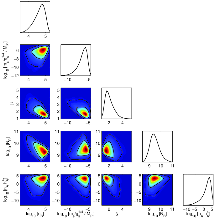
Figure 5: Solid lines show the marginalized 2D-joint 68% and 95% probability contours (off-diagonal panels) and 1D marginalized probability distribution (diagonal panels) for the microphysical IR DBI parameters. The color coding in the off-diagonal panels shows the marginalized probability density in these 2D parameter spaces, ranging from red for the highest density to blue for the lowest.

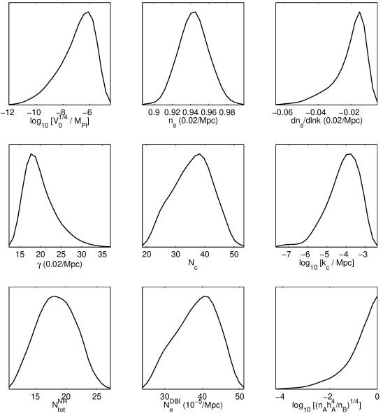
Figure 6: Marginalized posterior probability distribution functions obtained from the MCMC analysis for observables and derived quantities of interest. The functions are normalized such that the area under the curve is one.

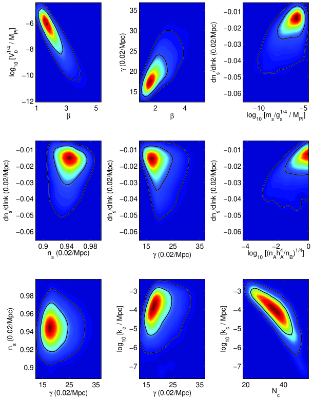
Figure 7: Examples of 2D contours. Solid lines show the marginalized 2D-joint 68% and 95% probability contours for observables and derived quantities of interest. The color coding shows the marginalized probability density in these 2D parameter spaces, ranging from red for the highest density to blue for the lowest.

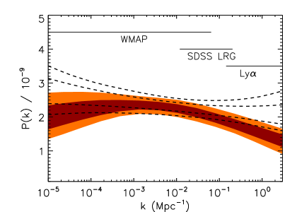
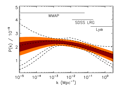
Figure 8: Reconstructed 68% (dark) and 95% (light) CL constraints on the primordial scalar power spectrum for the IR DBI model. The range of scales spanned by WMAP and SDSS LRG data (which were used in the fit) and the smaller scales covered by Lyman–$\alpha$ data (which were not) are shown for reference. For comparison, the dashed lines show the corresponding 68% and 95% constraints for (Upper) single-field slow-roll inflation, taken from Ref. [88] fitted to the WMAP and SDSS main galaxy sample data [4], and for (Lower) the empirical power law ansatz where the primordial power spectrum is described by its amplitude at a pivot scale, the spectral index $n_{s}$, and its running $dn_{s}/d\ln k$, fitted to WMAP, SDSS LRG and Supernova Legacy Survey [7] data. See text for discussion.

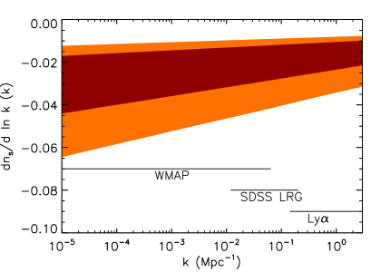
Figure 9: Reconstructed 68% (dark) and 95% (light) CL constraints on the scale-dependence of the running of the spectral index, $dn_{s}/d\ln k$, showing a mild indication for a “running of the running”. See text for discussion.

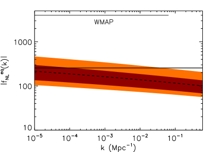
Figure 10: Reconstructed 68% (dark) and 95% (light) CL constraints and mean (dashed) for the non-linearity parameter $f_{NL}^{\rm eq}$ for the IR DBI model, as a function of scale. Note that DBI inflation predicts $f_{NL}^{\rm eq}<0$, and the absolute value is plotted for convenience. The range of scales spanned by WMAP data are shown, as well as the WMAP 95% lower limit $f_{NL}^{\rm eq}>-256$ (solid line), from an analysis which treated $f_{NL}^{\rm eq}$ as scale-independent [68]. See text for discussion.

5 Discussion and Conclusions

We conclude by highlighting the main results and discussing their physical implications. The quoted ranges are at the $95\%$ confidence level, and we have combined constraints from both the power spectrum and non-Gaussianity. The detailed $68\%$ and $95\%$ CL marginalized constraints and the maximum likelihood values are listed in Table 3.

5.1 Microscopic parameters

• Shape of the inflaton brane moduli potential: $1.3<\beta<3.7$. The lower bound is due to constraints from the power spectrum, while the upper bound is due to the non-Gaussianity constraint. It is encouraging that, while IR DBI inflation can happen for a range of $\beta$ that varies over nearly 10 orders of magnitude, $0.1\lesssim\beta<10^{9}$ (see Eq. (2.21)), comparison with data picks out a very small range around ${\cal O}(1)$ which is generically expected theoretically. This makes an explicit construction of such potentials a more interesting question.

• Fundamental string scale: $-9.6<\log_{10}(m_{s}/M_{\rm Pl})/g_{s}^{1/4}<-5.3$. The upper bound on the string scale is due to the large charge, and hence length scale, of the B-throat required to fit the amplitude of the density perturbations. The lower bound is due to the fact that a smaller string scale tends to increase the total number of $e$-folds of non-relativistic fast-roll inflation, and make the running of the spectral index too large (Fig. 7). The model prefers an intermediate fundamental string scale, $10^{8}\ {\rm GeV}<m_{s}/g_{s}^{1/4}<10^{13}\ {\rm GeV}$, and therefore an intermediate large volume compactification, $8.9\times 10^{7}<V^{1/6}M_{\rm Pl}<4.8\times 10^{13}$, where $V$ is the compactification volume.

• B-throat charge: $8.8<\log_{10}N_{B}<10.4$; Number of inflaton branes: $3.9<\log_{10}n_{B}<5.1$. In terms of the GKP-type warped compactification, this implies flux numbers $K\sim M\sim\sqrt{N_{B}}\sim{\cal O}(10^{5})$. Explicit construction remains an open question as discussed in Sec. 2.3. In the multi-throat brane inflation scenario, inflaton branes are generated from flux-antibrane annihilation. The number of branes generated in this process is roughly determined by the flux number $M$. Indeed, a small number of inflaton branes is ruled out by the data.

• A-throat minimum warp factor: $-2.4<\log_{10}h_{A}\leq 0$. This is from combining the constraint on $n_{B}$ and $n_{A}h_{A}^{4}$, $h_{A}=(n_{A}h_{A}^{4}/n_{B})^{1/4}$. A smaller $h_{A}$ leads to larger $N^{\rm NR}_{\rm tot}$ and larger running of the spectral index (Fig. 7). So the A-throat tends to be short. This makes tunneling reheating possible, where many interesting phenomena can occur, such as an intermediate matter-dominated epoch.

5.2 Secondary derived parameters

• Inflationary phases. In this model, not all $e$-folds comes from IR DBI inflation. The last $13<N^{\rm NR}_{\rm tot}<24$ $e$-folds come from non-relativistic fast-rolling inflation, which is possible because inflatons are close to the top of the potential.

• The stringy phase transition. The Hubble-expansion induced stringy phase transition happens at the largest scales in the sky, $-6.0<\log_{10}k_{c}/{\rm Mpc}<-2.9$. However its impact on density perturbations extends over to shorter scales, such as generating a transient large running of the spectral index.

• Inflation scale: $-10.0<\log_{10}V_{0}^{1/4}/M_{\rm Pl}<-5.1$. This gives a very small tensor to scalar ratio $r_{TS}<10^{-13}$.

• Cosmic string tension: $-23<\log_{10}G\mu_{D}+\log_{10}g_{s}^{1/2}<-14$. Here the cosmic strings refer to the D-strings left over from the brane-antibrane annihilation in the A-throat, whose tension is $G\mu_{D}=(m_{s}h_{A}/g_{s}^{1/4}M_{\rm Pl})^{2}/(16\pi^{2}g_{s}^{1/2})$. There is an unconstrained freedom coming from the additive factor $\log_{10}g_{s}^{1/2}$, but it is not expected to give any significant contributions. The F-string tension differs by a factor of $g_{s}$, $\mu_{F}=g_{s}\mu_{D}$.

5.3 Observational predictions

• Large, but regional, running of spectral index: $-0.046<dn_{s}/d\ln k(k=0.02/{\rm Mpc})<-0.010$. A reconstructed full-scale power spectrum and the running of the spectral index are shown in Fig. 8 & 9.

  This prediction is stringy in nature. A better understanding of the theoretical details and better measurements of both the power spectrum and non-Gaussianities on the relevant scales may reveal finer structures. In future experiments, Planck is expected to achieve $\sigma(dn_{s}/d\ln k)=0.005$ [9].

• Large non-Gaussianities: $-272<f_{NL}^{\rm eq}(k=0.02/{\rm Mpc})<-70$. A reconstructed full-scale prediction is in Fig. 10, which shows the running of the non-Gaussianities.

  This prediction is strictly speaking field-theoretic, but with strong string theory motivations, such as warped compactification and the DBI brane action. This field theoretic regime is $k>k_{c}$; the theoretical analysis for non-Gaussianities at $k\lesssim k_{c}$ is currently unavailable and remains an interesting open question. In future experiments, on CMB scales, Planck can achieve $\sigma(f^{\rm eq}_{NL})=67$ [92, 69]; on large scale structure scales, some high-$z$ galaxy surveys can reach similar or better precision [70].

As seen from these results, constraints from cosmological data, and even relatively loose constraints such as the non-Gaussianity constraint, are already putting strong restrictions on models which aim to provide self-consistent microphysical descriptions of the early universe. With the bounty of precision cosmological data expected in the future, the hope of probing not just field-theoretic, but string-theoretic early universe physics burns brightly.

Appendix A Estimate the effect of phase transition on spectral index

In this appendix we estimate the transition behavior of the spectral index between two asymptotic values described in Ref. [36, 39] and Sec. 3.2. Consider a simple model where the density perturbations are caused by the scalar field fluctuations, which are the super-horizon ripples on branes in transverse directions. These ripples are generated during a Hubble time while they are still sub-horizon and then frozen. The amplitude of the ripples are given by the fluctuation speed of a Hubble-sized patch on the brane. This speed is determined by the energy pumped into the branes by the Hubble expansion. This model simplifies the underlying physics by focusing on only the overall fluctuation speed of a Hubble-sized patch while ignoring the detailed world-volume theory such as effects from specific stringy excitations.

According to the special relativity, an object with rest mass $m_{0}$ and energy $E=m_{0}+\Delta E$ has velocity

$$v=c\sqrt{1-\frac{m_{0}^{2}}{(m_{0}+\Delta E)^{2}}}~{}.$$ (A.1)

For the on-brane observer, a Hubble-sized patch has rest mass

$$m_{0}=h_{B}^{4}T_{3}\Delta V=h_{B}^{4}T_{3}\left(\frac{\gamma H}{2\pi}\right)^{-3}~{},$$ (A.2)

where $h_{B}^{4}T_{3}$ is the red-shifted brane tension. The Hubble energy is $\gamma H/2\pi$, half of which goes to the kinetic energy of the transverse oscillation of the brane $\Delta E=\gamma H/4\pi$, while the other half goes to the tension of oscillations in terms of spatial derivatives. We have restored the factor of $2\pi$ in the Hubble length and energy in order to quantitatively match the known results in the low energy limit. The local speed of light is $c=h_{B}^{2}$. The position-dependent time delay is

$$\delta t=\frac{v(\gamma H/2\pi)^{-1}/\gamma}{\dot{r}\sqrt{n_{B}}}~{},$$ (A.3)

where the numerator is the fluctuation amplitude within a Hubble time viewed from the lab observer (hence an extra factor of $1/\gamma$ due to Lorentz contraction), and the denominator is the overall brane velocity which is approximately the local speed of light $\dot{r}\approx c$. Here we also consider the case of $n_{B}$ multiple branes where the superposition of independent fluctuations reduces the time-delay by a factor of $1/\sqrt{n_{B}}$. Using these estimates we obtain the power spectrum

$$P_{k}=\frac{4\pi^{2}v^{2}T_{3}}{\gamma^{4}\dot{\phi}^{2}}~{},$$ (A.4)

where

$$v^{2}T_{3}=h_{B}^{4}T_{3}\left[1-\left(1+\vphantom{\Biggl{(}}\displaystyle{\frac{\gamma^{4}H^{4}}{32\pi^{4}h_{B}^{4}T_{3}}}\right)^{-2}\right]~{}.$$ (A.5)

This formula recovers the usual field theory result in the limit of non-relativistic fluctuation speed. This includes non-relativistic-(slow or fast)-roll inflation, and DBI inflation below the phase transition. This formula also gives an estimate on the effect of the Hubble-expansion induced stringy phase transition. The estimate is expected to provide the envelope behavior beyond the transition since it ignores detailed features such as specific resonant production of various stringy states.

It will be useful to extract the DBI inflation region in (A.4) and (A.5), and parametrize it in the following way,

$$P_{k}=H^{2}\delta t^{2}=\frac{324\pi^{2}}{n_{B}\beta^{4}{N_{e}^{\rm DBI}}^{4}}\left(1-\frac{N_{c}^{16}}{(N_{c}^{8}+{N_{e}^{\rm DBI}}^{8})^{2}}\right)~{}.$$ (A.6)

$N_{c}$ is defined as

$$N_{c}\equiv 2^{5/8}\sqrt{3\pi}\frac{\lambda_{B}^{1/8}}{n_{B}^{1/8}\beta^{1/2}}=\sqrt{6}\pi^{1/4}\frac{N_{B}^{1/8}}{\beta^{1/2}}~{},$$ (A.7)

where we have used the relation (2.3). Taking the limits $N_{e}\ll N_{c}$ and $N_{e}\gg N_{c}$, we recover (3.13) and (3.18) respectively. The spectral index is

$$n_{s}-1=\frac{4}{N_{e}^{\rm DBI}}\frac{x^{2}+3x-2}{(x+1)(x+2)}~{},~{}~{}~{}~{}x\equiv\left(\frac{N_{e}^{\rm DBI}}{N_{c}}\right)^{8}~{}.$$ (A.8)

This formula interpolates between two asymptotic values $4/N_{e}$ and $-4/N_{e}$. If we define the width of the transition region as the $e$-fold difference $\Delta N_{e}$ between $n_{s}-1=2/N_{e}^{\rm DBI}$ and $-2/N_{e}^{\rm DBI}$, then we have

$$\Delta N_{e}\approx 0.2N_{c}~{},$$ (A.9)

which can be quite large (for example, six if $N_{c}=30$). But the running of $n_{s}$ is still observably large in the transition region (for example, $dn_{s}/d\ln k\approx-0.02$ in the range of (A.9) for $N_{c}=30$).

Appendix B Running spectral index from slow-roll potential with mild features

Usual slow-roll inflation gives negligible running of the spectral index, $dn_{s}/d\ln k={\cal O}(10/N_{e}^{2})$, because large running of $n_{s}$ tends to end the inflation too quickly. For a comparison with data, see Ref. [93]. In this appendix, we study the possibility of having measurable $|dn_{s}/d\ln k|\gtrsim 0.01$ by adding some mild features to the slow-roll potential, and how we can phenomenologically distinguish it from the IR DBI inflation model.

We consider a potential of a small field inflation and add some ripples on it,

$$V=V_{0}-a\phi-b\sin(\phi/\phi_{0})~{}.$$ (B.1)

The inflaton starts for example at $\phi_{i}=0$. At $\phi=\phi_{\rm end}$, one imagines that the inflationary energy $V_{0}$ gets annihilated as in brane-anti-brane inflation. This is just an example of many possibilities, which we use to illustrate the main properties. As we will see, to generate a large running of $n_{s}$ from blue to red, the shape of the slow-roll potential changes from convex to concave. The oscillatory ripples help to sustain inflation, and at the same time generate large $dn_{s}/d\ln k$ periodically. In fact, for our purpose, it is not necessary to make the mild feature periodic, for example the 3rd term in (B.1) can be regional as long as it falls into the WMAP range. Nonetheless being periodic might be more naturally realized in model-building.

We want the inflaton to continuously roll down, so we need $V^{\prime}\leq 0$, i.e. ,

$$-a+b/\phi_{0}\leq 0~{}.$$ (B.2)

We require the average slow-roll parameter

$$\epsilon=\frac{M_{\rm Pl}^{2}}{2}\frac{a^{2}}{V_{0}^{2}}\ll 1$$ (B.3)

to have enough inflationary $e$-folds. To have the effect of one ripple span several $e$-folds, we need $\phi_{0}/\dot{\phi}=\xi H^{-1}$, where $\xi$ is of order one. $\dot{\phi}$ can be estimated using the attractor behavior $3H\dot{\phi}+V^{\prime}=0$ and taking the average value of $V^{\prime}$. We want the other slow-roll parameter $\eta$ to vary between order $\pm 0.1$ to generate observable $dn_{s}/d\ln k$,

$$|\eta|\leq M_{\rm Pl}^{2}\frac{b}{\phi_{0}^{2}V_{0}}\equiv\zeta~{},$$ (B.4)

where $\zeta$ is ${\cal O}(0.1)$.

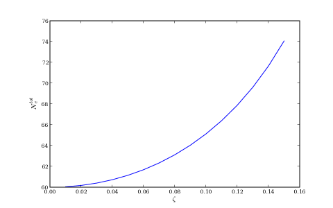
Figure 11: Turning on the periodic mild features $\zeta$ does not significantly affect the total inflationary $e$-folds. In this figure, $\xi=4$, $a/V_{0}=10^{-4}$, $\phi$ starts from $0$ and ends at $0.006M_{\rm Pl}$.

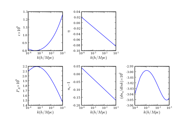
Figure 12: The power spectrum and spectral index in the WMAP range for a slow-roll potential with mild features. The parameters $a/V_{0}=10^{-4}$, $\xi=4$ and $\zeta=0.15$ are chosen so that these observables look close to what we obtained in the IR DBI model.

Therefore for our purpose, we can choose the parameters in (B.1) in the following way. We require

$$a\ll\frac{V_{0}}{M_{\rm Pl}}$$ (B.5)

so that $\epsilon\ll 1$;

$$\phi_{0}=\xi\frac{aM_{\rm Pl}^{2}}{V_{0}}$$ (B.6)

with $\xi$ of ${\cal O}(1)$ so that the effect of one period of the mild feature spans a reasonable amount of $e$-folds;

$$b=\xi^{2}\zeta\frac{a^{2}M_{\rm Pl}^{2}}{V_{0}}$$ (B.7)

with $\zeta$ of ${\cal O}(0.1)$ so that the running of $n_{s}$ is observably large. In order for these conditions to be consistent with (B.2), we need

$$\xi\zeta\leq 1~{}.$$ (B.8)

For example, we can choose $\xi=4$, $\zeta=0.15$.

In Fig. 11 and 12 we demonstrate numerically:

• Introducing such mild features does not significantly affect, and in fact can slightly increase, the total number of inflationary $e$-folds.

• The power spectrum within the WMAP scales looks like what we obtained in IR DBI model; notably, the spectral index runs from blue to red with a large and negative $dn_{s}/d\ln k$.

To experimentally distinguish this case from the IR DBI model, we estimate the non-Gaussianity. In slow-roll inflation, the 3-point function of the gauge-invariant scalar perturbation receives contributions from the following sources [71, 94]. In the cubic action there are terms proportional to $\epsilon^{2}$, $\epsilon^{3}$ and $\epsilon d\eta/dt$. In terms of order-of-magnitude, these terms contribute ${\cal O}(\epsilon)$, ${\cal O}(\epsilon^{2})$, ${\cal O}(\Delta\eta)$, respectively, to the non-Gaussianity estimator $f_{NL}$. The $\Delta\eta$ is the maximum change of $\eta$ caused by the features, since the 3-point function involves an integration over time. In addition, there is a field redefinition term that contributes ${\cal O}(\eta_{\rm end})$ to $f_{NL}$, where $\eta_{\rm end}$ is the frozen value of $\eta$ after the horizon crossing.

In case of slow-roll inflation with smooth potential, the leading terms of $f_{NL}$ are ${\cal O}(\epsilon)$ and ${\cal O}(\eta)$ [71]. In case of sharp features, ${\cal O}(\Delta\eta)$ term dominates [30]. In the case of interest here with periodic mild features, both ${\cal O}(\Delta\eta)$ and the boundary term ${\cal O}(\eta_{\rm end})$ become important. As we saw, to generate large but reasonable running of the spectral index, we require $\eta$ to vary between $\pm{\cal O}(0.1)$. So we expect such features to be associated with non-Gaussianities $f_{NL}={\cal O}(0.1)$. This is clearly observationally distinguishable from the IR DBI inflation case.

Appendix C Running spectral index from non-Bunch-Davies vacuum

In this Appendix, we study how the running spectral index arising from the non-Bunch-Davies vacuum case can be phenomenologically distinguished from the running spectral index in IR DBI model.

In the field theory of density perturbations, the Bunch-Davies (BD) vacuum is the leading behavior of the fluctuations when they are well within the horizon. However corrections to such a vacuum can have observational effects and may provide information on new physics [95]. For reviews and references see [96, 97]. Denoting the scale of the new physics as $M\gg H$, this correction typically arises at the order $H/M$, for example, if we choose the adiabatic vacuum at the scale $M$ [98]. This is also called the trans-Planckian effect if $M$ is regarded as $M_{\rm Pl}$. In this appendix, we will treat $M$ to be much more general.

The main difference between the case of non-BD vacuum and the Hubble-expansion induced stringy phase transition in DBI inflation is that, in the former, there is a large region between the new physics scale and the Hubble horizon where the conventional field theoretic analyses still applies; while in the latter, the Hubble horizon is comparable to or smaller than the new stringy length scale in the inflaton sector.

The effect of non-Bunch-Davies vacuum in slow-roll inflation typically results in an oscillatory modulation on the usual power spectrum [99, 100]. So it may also introduce an observable running spectral index. The potential for observing these features are discussed in Ref. [101, 102]. To study both slow-roll and DBI inflation, here we generalize the analyses of Ref. [98, 103] to the case with arbitrary sound speed.

The quadratic action for the gauge-invariant scalar perturbation $\zeta$ in general single field inflation is

$$S_{2}=\int dtd^{3}x\left[a^{3}\frac{\epsilon}{c_{s}^{2}}\dot{\zeta}^{2}-a\epsilon(\partial\zeta)^{2}\right]~{},$$ (C.1)

where $a$ is the scale factor, $c_{s}$ is the sound speed, and $\epsilon=-\dot{H}/H^{2}$ is one of the slow variation parameters. Using the variable $v_{\bf k}\equiv z\zeta_{\bf k}$ ($z\equiv a\sqrt{2\epsilon}/c_{s}$) and its conjugate momentum

$$\pi_{\bf k}=v^{\prime}_{\bf k}-\frac{z^{\prime}}{z}v_{\bf k}~{},$$ (C.2)

the Hamiltonian in Fourier space is

$$H_{2}=\frac{1}{(2\pi)^{3}}\int d^{3}k\frac{1}{2}\left[\pi_{\bf k}\pi^{*}_{\bf k}+k^{2}c_{s}^{2}v_{\bf k}v^{*}_{\bf k}+\frac{z^{\prime}}{z}(\pi_{\bf k}v^{*}_{\bf k}+\pi^{*}_{\bf k}v_{\bf k})\right]~{},$$ (C.3)

where the prime denotes the derivative with respective to the conformal time $\tau$.

We can quantize $v_{\bf k}$ and $\pi_{\bf k}$ in terms of the creation and annihilation operators which are either time-dependent

$$v_{\bf k} = \frac{1}{\sqrt{2kc_{s}}}\left(a_{\bf k}(\tau)+a^{\dagger}_{-{\bf k}}(\tau)\right)~{},$$

$$\pi_{\bf k} = -i\sqrt{\frac{kc_{s}}{2}}\left(a_{\bf k}(\tau)-a^{\dagger}_{-{\bf k}}(\tau)\right)~{},$$ (C.4)

or time-independent

$$v_{\bf k} = f_{k}(\tau)a_{\bf k}(\tau_{0})+f_{k}^{*}(\tau)a^{\dagger}_{-{\bf k}}(\tau_{0})~{},$$

$$\pi_{\bf k} = -i\left[g_{k}(\tau)a_{\bf k}(\tau_{0})-g^{*}_{k}(\tau)a^{\dagger}_{-{\bf k}}(\tau_{0})\right]~{},$$ (C.5)

where $f_{k}(\tau)$ is the solution of the equation of motion $v_{\bf k}^{\prime\prime}+c_{s}^{2}k^{2}v_{\bf k}-(z^{\prime\prime}/z)v_{\bf k}=0$,

$$f_{k}(\tau) = C_{+}\frac{1}{\sqrt{2c_{s}k}}\left(1-\frac{i}{kc_{s}\tau}\right)e^{-ikc_{s}\tau}+C_{-}\frac{1}{\sqrt{2c_{s}k}}\left(-1-\frac{i}{kc_{s}\tau}\right)e^{ikc_{s}\tau}~{},$$

$$g_{k}(\tau) = C_{+}\sqrt{\frac{kc_{s}}{2}}e^{-ikc_{s}\tau}+C_{-}\sqrt{\frac{kc_{s}}{2}}e^{ikc_{s}\tau}~{}.$$ (C.6)

Equations (C.4) and (C.5) are related by the Bogolubov transformation

$$a_{\bf k}(\tau) = \xi_{k}(\tau)a_{\bf k}(\tau_{0})+\zeta_{k}(\tau)a^{\dagger}_{-{\bf k}}(\tau_{0})~{},$$

$$a^{\dagger}_{-{\bf k}}(\tau) = \xi^{*}_{k}(\tau)a^{\dagger}_{-{\bf k}}(\tau_{0})+\zeta_{k}^{*}(\tau)a_{\bf k}(\tau_{0})~{},$$ (C.7)

where

$$\xi_{k} = \sqrt{\frac{kc_{s}}{2}}f_{k}+\sqrt{\frac{1}{2kc_{s}}}g_{k}~{},$$

$$\zeta_{k} = \sqrt{\frac{kc_{s}}{2}}f^{*}_{k}-\sqrt{\frac{1}{2kc_{s}}}g^{*}_{k}~{}.$$ (C.8)

The following relation should be satisfied to preserve the commutation relation for (C.7),

$$|\xi_{k}|^{2}-|\zeta_{k}|^{2}=1.$$ (C.9)

Therefore we have $f_{k}g_{k}^{*}+f_{k}^{*}g_{k}=1$ and $|C_{+}|^{2}-|C_{-}|^{2}=1$.

An adiabatic vacuum $|0,\tau_{0}\rangle$ can be chosen as

$$a_{\bf k}(\tau_{0})|0,\tau_{0}\rangle=0~{},~{}~{}~{}~{}{\rm{\it{i.e.}}}~{}~{}~{}\zeta_{k}(\tau_{0})=0~{}.$$ (C.10)

The Bunch-Davies vacuum corresponds to sending $\tau_{0}$ to $-\infty$. More generally one can choose a finite $\tau_{0}\approx-1/a_{0}H_{0}$ for the mode ${\bf k}$, when this mode crosses the scale of the new physics $M\gg H/c_{s}$. Hence the relation between the power spectrum in the non-BD and BD vacuum is

$$P_{k}^{\rm nonBD}=|C_{+}+C_{-}|^{2}P_{k}^{\rm BD}~{},$$ (C.11)

where

$$|C_{+}+C_{-}|^{2} \approx 1-\left(\frac{aH}{kc_{s}}\right)_{\tau}\sin\left(\frac{2kc_{s}}{aH}\right)_{\tau}~{},$$ (C.12)

$$\approx 1-\left(\frac{H}{Mc_{s}}\right)_{\tau}\sin\left(\frac{2Mc_{s}}{H}\right)_{\tau}~{},$$

where the new physics scale $M=(k/a)_{\tau}$. The extra contribution of the non-BD vacuum to the spectral index is

$$\Delta n_{s}\approx-2(\epsilon+s+\mu)\cos\frac{2Mc_{s}}{H}~{},$$ (C.13)

where $\mu\equiv\dot{M}/(HM)$, $s\equiv\dot{c}_{s}/(Hc_{s})$. In the following discussion, we will concentrate on the amplitude and oscillation frequency of these features on the power spectrum and spectral index. We want to compare them to those in IR DBI model, where the spectral index $n_{s}-1$ changes between $\pm{\cal O}(0.1)$ within ${\cal O}(10)$ $e$-folds without oscillations. For this purpose it is useful to note that the change of the arguments in the trigonometric functions in (C.11) and (C.13) as a function of $k$ can be written as

$$\Delta\left(\frac{2Mc_{s}}{H}\right)_{\tau}=\left(\frac{2Mc_{s}}{H}\right)_{\tau_{0}}(\epsilon+s+\mu)\ln\frac{k}{k_{0}}~{}.$$ (C.14)

We first look at slow-roll inflation, where $s=\mu=0$ and $\epsilon\lesssim 0.01$. So the variation of $n_{s}$, typically smaller than ${\cal O}(0.01)$, is much smaller than that caused by the phase transition in IR DBI case, although the oscillatory frequency of the $n_{s}$ is adjustable depending on the values of $(2M/H)_{\tau_{0}}$ and $\epsilon$. For $n_{s}$ to have larger variations, one needs the special case of $\epsilon\approx 0.05$; at the same time, for the running to span ${\cal O}(10)$ $e$-folds without oscillation, from (C.14), we see that $Mc_{s}/H={\cal O}(\pi)$. This barely satisfies $Mc_{s}/H\gg 1$. We conclude that in slow-roll inflation the effect of the non-DB vacuum on $n_{s}$, having much smaller $\Delta n_{s}$ or large oscillatory frequencies, will be observationally distinguishable from that caused by the phase transition in IR DBI inflation. In addition, there are no observable non-Gaussianities associated with them.

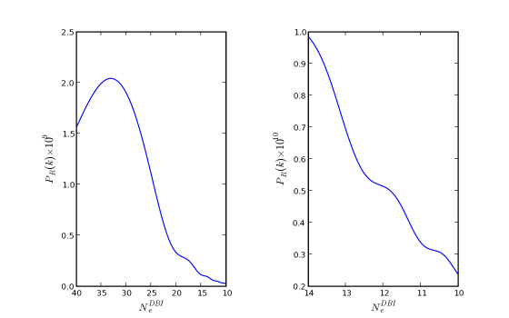
Figure 13: Illustration of the effect of the non-BD vacuum and the stringy phase transition in IR DBI model, combining (A.6) and (C.11). We use $N_{c}\sim 40$, which is also the scale where $M\sim H/c_{s}$. The ripples at small scales are due to the non-BD effects and the suppression in large scales is due to the phase transition. The connection between them is smoothed out by hand due to a lack of more detailed understanding. The right panel is a blow-up of the left.

We next look at the effect of the non-BD vacuum on the IR DBI inflation. Now $\epsilon$ is negligibly small and $s=1/N_{e}^{\rm DBI}$. The natural scale of $M$ is the red-shifted string scale, so $M\propto 1/N_{e}^{\rm DBI}$ and $\mu=1/N_{e}^{\rm DBI}$. As we see from Sec. 3.1, $N_{e}^{\rm DBI}$ is typically smaller than $N_{e}$. So the variation of $n_{s}$ can be comparable to ${\cal O}(0.1)$. Using (C.14), over ${\cal O}(10)$ $e$-folds the change of the arguments in the trigonometric function is $2Mc_{s}/H\gg 1$, so the modulation is oscillating rapidly. In fact since the larger scales are associated with smaller $M$ during inflation, by the time that the modulation stops oscillating, we have $M\sim H/c_{s}$. This is already beyond the validity region of the non-BD vacuum calculations, and in fact is the place where the stringy phase transition takes effect. So we conclude that, in IR DBI model, the effect of the non-BD vacuum is smoothly connected to the phase transition. Phenomenologically they look different from the phase transition by causing frequent oscillations in the spectral index. In Fig. 13 we illustrate this effect on the power spectrum. The amplitude of the oscillatory modulation increases and the frequency decreases towards the large scales, and finally merges into the phase transition.

The effect of the non-BD vacuum on the large non-Gaussianities in DBI inflation is studied in [66]. The distinctive signature is the rising behavior in the shape of the 3-point function in the folded triangle limit. This may also be an interesting clue to a better understanding of the properties of the non-Gaussianity during the phase transition.

Appendix D Details of numerical calculations

The zero mode motion of the brane in a warped throat is captured by the DBI-CS action (3.1). Varying the action, the exact form of the equations of motion is given by,

$$\phi_{NN} = -\frac{3}{2}\frac{f^{\prime}}{f}\phi_{N}^{2}-\left(\frac{H_{N}}{H}+\frac{3}{\gamma^{2}}\right)\phi_{N}+\frac{f^{\prime}}{f^{2}H^{2}}-\frac{1}{\gamma^{3}H^{2}}\left(V^{\prime}+\frac{f^{\prime}}{f^{2}}\right)~{},$$ (D.1)

$$H_{N} = -\frac{1}{2}\gamma H\phi_{N}^{2}~{},$$ (D.2)

$$\gamma = \left[1-f(\phi)H^{2}\phi_{N}^{2}\right]^{-1/2}~{},$$ (D.3)

$$f(\phi) = \frac{\lambda}{\phi^{4}},\quad\lambda\equiv n_{B}T_{3}R_{B}^{4}~{}.$$ (D.4)

In the above differential equations, we choose to use the number of $e$-folds $\tilde{N}_{e}=\ln a(t)$ as the time coordinate, as the intrinsic time scale of inflationary dynamics is the Hubble time $H^{-1}$. The subscript _N denotes derivatives with respect to $\tilde{N}_{e}$, i.e. $\phi_{N}\equiv d\phi/d\tilde{N}_{e}$, $\phi_{NN}\equiv d^{2}\phi/d\tilde{N}_{e}^{2}$. We also denote derivatives with respect to $\phi$ by a prime, i.e. $f^{\prime}\equiv df/d\phi$, $V^{\prime}\equiv dV/d\phi$.

The equations (D.1) and (D.2) can be integrated numerically using the conventional Runge-Kutta method. We note that ignoring Eq. (D.2) and setting $H_{N}/H=0$ in Eq. (D.1) does not introduce detectable errors to the results of numerical calculation, because $H$ can safely be treated as a constant for IR DBI inflation. Nevertheless, we have put Eq. (D.2) through numerical integration together with (D.1) for self-consistency.

To integrate the equation of motion, the code needs to know the initial values $\phi(0)$ and $\phi_{N}(0)$. Due to the attractor behavior of the IR DBI dynamics, these initial conditions will be irrelevant to our calculation of observables as long as inflation lasts a few $e$-folds more than the minimum number required to solve the horizon problem. This can always be done in the IR DBI model, since we have the freedom to extend the start of inflation to the IR end of the throat by choosing $\phi(0)$ appropriately. In practice, we choose $\phi(0)<H\sqrt{\lambda_{B}}/80$, so that according to (3.3), we will have at least 80 DBI $e$-folds, and roughly 90 total $e$-folds (assuming 10 non-relativistic $e$-folds). This is good enough to make sure that, when we calculate primordial density perturbations on scales relevant to CMB temperature anisotropies (roughly $50\sim 60$ $e$-folds before the end of inflation), the inflationary background is well on the attractor solution.

To set up the model, the numerical code needs the five microscopic parameters $\{N_{B}$, $n_{B}$, $n_{A}h_{A}^{4}$, $g_{s}^{-1/4}m_{s}$, $\beta\}$. The five input parameters need to satisfy various bounds for model building consistency. The following microphysical bounds are imposed in the code:

• the geometric constraint from compactification (Eq. (3.32))

  $$\frac{m_{s}}{g_{s}^{1/4}}\lesssim 2^{3/2}\pi^{11/4}a_{B}^{1/2}\frac{M_{\rm Pl}}{N_{B}^{3/4}}~{};$$

• the maximum number of branes generated by antibrane-flux annihilation (Eq. (3.31))

  $$n_{B}\lesssim\sqrt{N_{B}/(a_{B}g_{s})}~{};$$

• the lower bound on string scale

  $$m_{s}g_{s}^{-1/4}\geq{\rm TeV}~{};$$

• the lower bound on inflation scale

  $$n_{A}h_{A}^{4}T_{3}\geq{\rm TeV}^{4}~{};$$

• the warp factor $h_{A}\leq 1$,

  $$n_{A}h_{A}^{4}\leq n_{B}~{}.$$

(In these bounds, we fix the string coupling $g_{s}=0.1$ and $a_{B}=1$. The effects of different $g_{s}$ and $a_{B}$ are discussed in Sec. 3.5.) Before calculating the density perturbation, the code performs checks on all of the above bounds to make sure the input parameters are theoretically consistent.

After numerically integrating the inflaton equation of motion, our immediate result is $\phi(\tilde{N}_{e})$, $\gamma(\tilde{N}_{e})$ and $H(\tilde{N}_{e})$. Then we use (3.28) to calculate the curvature perturbation $P_{R}(\tilde{N}_{e})$ generated during inflation. Once we have $P_{R}(\tilde{N}_{e})$, the horizon crossing relation (3.30) can translate $P_{R}(\tilde{N}_{e})$ to $P_{R}(k)$, (noting $N_{e}=N_{\rm tot}-\tilde{N}_{e}$,) which is then fed into CAMB to generate the CMB temperature anisotropy spectrum and the matter power spectrum.

References

- [1]
- [2] D. N. Spergel et al. [WMAP Collaboration], “Wilkinson Microwave Anisotropy Probe (WMAP) three year results: Implications for cosmology,” arXiv:astro-ph/0603449.
- [3] D. G. York et al. [SDSS Collaboration], “The Sloan Digital Sky Survey: technical summary,” Astron. J. 120, 1579 (2000) [arXiv:astro-ph/0006396].
- [4] M. Tegmark et al. [SDSS Collaboration], “The 3D power spectrum of galaxies from the SDSS,” Astrophys. J. 606, 702 (2004) [arXiv:astro-ph/0310725].
- [5] M. Tegmark et al., “Cosmological Constraints from the SDSS Luminous Red Galaxies,” Phys. Rev. D 74, 123507 (2006) [arXiv:astro-ph/0608632].
- [6] P. McDonald et al. [SDSS Collaboration], “The Linear Theory Power Spectrum from the Lyman-alpha Forest in the Sloan Digital Sky Survey,” Astrophys. J. 635, 761 (2005) [arXiv:astro-ph/0407377].
- [7] P. Astier et al. [The SNLS Collaboration], “The Supernova Legacy Survey: Measurement of , and from the First Year Data Set,” Astron. Astrophys. 447, 31 (2006) [arXiv:astro-ph/0510447].
- [8] C. L. Kuo et al., “Improved Measurements of the CMB Power Spectrum with ACBAR,” arXiv:astro-ph/0611198.
- [9] The Planck Bluebook: http://www.rssd.esa.int/index.php?project=Planck
- [10] http://www.physics.princeton.edu/act/
- [11] http://www.astro.caltech.edu/ lgg/spider_front.htm
- [12] A. H. Guth, “The Inflationary Universe: A Possible Solution To The Horizon And Flatness Problems,” Phys. Rev. D 23, 347 (1981).
- [13] A. D. Linde, “A New Inflationary Universe Scenario: A Possible Solution Of The Horizon, Flatness, Homogeneity, Isotropy And Primordial Monopole Problems,” Phys. Lett. B 108, 389 (1982).
- [14] A. Albrecht and P. J. Steinhardt, “Cosmology For Grand Unified Theories With Radiatively Induced Symmetry Breaking,” Phys. Rev. Lett. 48, 1220 (1982).
- [15] G. R. Dvali and S. H. H. Tye, “Brane inflation,” Phys. Lett. B 450, 72 (1999) [arXiv:hep-ph/9812483].
- [16] S. H. Henry Tye, “Brane inflation: String theory viewed from the cosmos,” arXiv:hep-th/0610221.
- [17] C. P. Burgess, “Lectures on Cosmic Inflation and its Potential Stringy Realizations,” arXiv:0708.2865 [hep-th].
- [18] A. Linde, “Inflationary Cosmology,” arXiv:0705.0164 [hep-th].
- [19] R. Kallosh, “On Inflation in String Theory,” arXiv:hep-th/0702059.
- [20] J. M. Cline, “String cosmology,” arXiv:hep-th/0612129.
- [21] C. P. Burgess, M. Majumdar, D. Nolte, F. Quevedo, G. Rajesh and R. J. Zhang, “The inflationary brane-antibrane universe,” JHEP 0107, 047 (2001) [arXiv:hep-th/0105204].
- [22] G. R. Dvali, Q. Shafi and S. Solganik, “D-brane inflation,” arXiv:hep-th/0105203.
- [23] S. Kachru, R. Kallosh, A. Linde, J. Maldacena, L. McAllister and S. P. Trivedi, “Towards inflation in string theory,” JCAP 0310, 013 (2003) [arXiv:hep-th/0308055].
- [24] M. R. Douglas and S. Kachru, “Flux compactification,” arXiv:hep-th/0610102.
- [25] D. H. Lyth and A. Riotto, “Particle physics models of inflation and the cosmological density perturbation,” Phys. Rept. 314, 1 (1999) [arXiv:hep-ph/9807278].
- [26] R. Bean, S. E. Shandera, S. H. H. Tye and J. Xu, “Comparing brane inflation to WMAP,” arXiv:hep-th/0702107.
- [27] J. A. Adams, B. Cresswell and R. Easther, “Inflationary perturbations from a potential with a step,” Phys. Rev. D 64, 123514 (2001) [arXiv:astro-ph/0102236].
- [28] H. V. Peiris et al. [WMAP Collaboration], “First year Wilkinson Microwave Anisotropy Probe (WMAP) observations: Implications for inflation,” Astrophys. J. Suppl. 148, 213 (2003) [arXiv:astro-ph/0302225].
- [29] L. Covi, J. Hamann, A. Melchiorri, A. Slosar and I. Sorbera, “Inflation and WMAP three year data: Features have a future!,” Phys. Rev. D 74, 083509 (2006) [arXiv:astro-ph/0606452].
- [30] X. Chen, R. Easther and E. A. Lim, “Large non-Gaussianities in single field inflation,” arXiv:astro-ph/0611645.
- [31] G. Hailu and S. H. Tye, “Structures in the Gauge/Gravity Duality Cascade,” arXiv:hep-th/0611353.
- [32] J. Polchinski, “Introduction to cosmic F- and D-strings,” arXiv:hep-th/0412244.
- [33] E. Silverstein and D. Tong, “Scalar speed limits and cosmology: Acceleration from D-cceleration,” Phys. Rev. D 70, 103505 (2004) [arXiv:hep-th/0310221].
- [34] M. Alishahiha, E. Silverstein and D. Tong, “DBI in the sky,” Phys. Rev. D 70, 123505 (2004) [arXiv:hep-th/0404084].
- [35] X. Chen, “Multi-throat brane inflation,” Phys. Rev. D 71, 063506 (2005) [arXiv:hep-th/0408084].
- [36] X. Chen, “Inflation from warped space,” JHEP 0508, 045 (2005) [arXiv:hep-th/0501184].
- [37] S. B. Giddings, S. Kachru and J. Polchinski, “Hierarchies from fluxes in string compactifications,” Phys. Rev. D 66, 106006 (2002) [arXiv:hep-th/0105097].
- [38] H. V. Peiris, D. Baumann, B. Friedman and A. Cooray, “Phenomenology of D-Brane Inflation with General Speed of Sound,” arXiv:0706.1240 [astro-ph].
- [39] X. Chen, “Running non-Gaussianities in DBI inflation,” Phys. Rev. D 72, 123518 (2005) [arXiv:astro-ph/0507053].
- [40] X. Chen, S. Sarangi, S. H. Henry Tye and J. Xu, “Is brane inflation eternal?,” JCAP 0611, 015 (2006) [arXiv:hep-th/0608082].
- [41] D. Baumann and L. McAllister, “A microscopic limit on gravitational waves from D-brane inflation,” arXiv:hep-th/0610285.
- [42] L. Randall and R. Sundrum, “A large mass hierarchy from a small extra dimension,” Phys. Rev. Lett. 83, 3370 (1999) [arXiv:hep-ph/9905221].
- [43] S. E. Shandera and S. H. Tye, “Observing brane inflation,” JCAP 0605, 007 (2006) [arXiv:hep-th/0601099].
- [44] J. E. Lidsey and I. Huston, “Gravitational wave constraints on Dirac-Born-Infeld inflation,” JCAP 0707, 002 (2007) [arXiv:0705.0240 [hep-th]].
- [45] J. E. Lidsey and D. Seery, “Primordial non-Gaussianity and gravitational waves: Observational tests of brane inflation in string theory,” Phys. Rev. D 75, 043505 (2007) [arXiv:astro-ph/0610398].
- [46] M. Spalinski, “A consistency relation for power law inflation in DBI models,” Phys. Lett. B 650, 313 (2007) [arXiv:hep-th/0703248].
- [47] L. Lorenz, J. Martin and C. Ringeval, “Brane inflation and the WMAP data: a Bayesian analysis,” arXiv:0709.3758 [hep-th].
- [48] R. A. Battye, B. Garbrecht, A. Moss and H. Stoica, “Constraints on Brane Inflation and Cosmic Strings,” arXiv:0710.1541 [astro-ph].
- [49] T. Kobayashi, S. Mukohyama and S. Kinoshita, “Constraints on Wrapped DBI Inflation in a Warped Throat,” arXiv:0708.4285 [hep-th].
- [50] M. Becker, L. Leblond and S. E. Shandera, “Inflation from Wrapped Branes,” arXiv:0709.1170 [hep-th].
- [51] S. Kachru, J. Pearson and H. L. Verlinde, “Brane/flux annihilation and the string dual of a non-supersymmetric field theory,” JHEP 0206, 021 (2002) [arXiv:hep-th/0112197].
- [52] X. Chen and S. H. Tye, “Heating in brane inflation and hidden dark matter,” JCAP 0606, 011 (2006) [arXiv:hep-th/0602136].
- [53] X. Chen, “Cosmological rescaling through warped space,” Phys. Rev. D 71, 026008 (2005) [arXiv:hep-th/0406198].
- [54] I. R. Klebanov and M. J. Strassler, “Supergravity and a confining gauge theory: Duality cascades and chiSB-resolution of naked singularities,” JHEP 0008, 052 (2000) [arXiv:hep-th/0007191].
- [55] S. Kecskemeti, J. Maiden, G. Shiu and B. Underwood, “DBI inflation in the tip region of a warped throat,” JHEP 0609, 076 (2006) [arXiv:hep-th/0605189].
- [56] G. Shiu and B. Underwood, “Observing the Geometry of Warped Compactification via Cosmic Inflation,” Phys. Rev. Lett. 98, 051301 (2007) [arXiv:hep-th/0610151].
- [57] S. Thomas and J. Ward, “IR Inflation from Multiple Branes,” Phys. Rev. D 76, 023509 (2007) [arXiv:hep-th/0702229].
- [58] X. Chen, Unpublished notes.
- [59] M. Berg, M. Haack and B. Kors, “Loop corrections to volume moduli and inflation in string theory,” Phys. Rev. D 71, 026005 (2005) [arXiv:hep-th/0404087].
- [60] D. Baumann, A. Dymarsky, I. R. Klebanov, J. Maldacena, L. McAllister and A. Murugan, “On D3-brane potentials in compactifications with fluxes and wrapped D-branes,” JHEP 0611, 031 (2006) [arXiv:hep-th/0607050].
- [61] C. P. Burgess, J. M. Cline, K. Dasgupta and H. Firouzjahi, “Uplifting and inflation with D3 branes,” JHEP 0703, 027 (2007) [arXiv:hep-th/0610320].
- [62] A. Krause and E. Pajer, “Chasing Brane Inflation in String-Theory,” arXiv:0705.4682 [hep-th].
- [63] D. Baumann, A. Dymarsky, I. R. Klebanov and L. McAllister, “Towards an Explicit Model of D-brane Inflation,” arXiv:0706.0360 [hep-th].
- [64] A. Klemm, B. Lian, S. S. Roan and S. T. Yau, “Calabi-Yau fourfolds for M- and F-theory compactifications,” Nucl. Phys. B 518, 515 (1998) [arXiv:hep-th/9701023].
- [65] J. Garriga and V. F. Mukhanov, “Perturbations in k-inflation,” Phys. Lett. B 458, 219 (1999) [arXiv:hep-th/9904176].
- [66] X. Chen, M. x. Huang, S. Kachru and G. Shiu, “Observational signatures and non-Gaussianities of general single field inflation,” JCAP 0701, 002 (2007) [arXiv:hep-th/0605045].
- [67] D. Babich, P. Creminelli and M. Zaldarriaga, “The shape of non-Gaussianities,” JCAP 0408, 009 (2004) [arXiv:astro-ph/0405356].
- [68] P. Creminelli, L. Senatore, M. Zaldarriaga and M. Tegmark, “Limits on parameters from WMAP 3yr data,” arXiv:astro-ph/0610600.
- [69] C. Hikage, E. Komatsu and T. Matsubara, “Primordial Non-Gaussianity and Analytical Formula for Minkowski Functionals of the Cosmic Microwave Background and Large-scale Structure,” Astrophys. J. 653, 11 (2006) [arXiv:astro-ph/0607284].
- [70] E. Sefusatti and E. Komatsu, “The bispectrum of galaxies from high-redshift galaxy surveys: primordial non-Gaussianity and non-linear galaxy bias,” arXiv:0705.0343 [astro-ph].
- [71] J. M. Maldacena, “Non-Gaussian features of primordial fluctuations in single field inflationary models,” JHEP 0305, 013 (2003) [arXiv:astro-ph/0210603].
- [72] E. Komatsu and D. N. Spergel, “Acoustic signatures in the primary microwave background bispectrum,” Phys. Rev. D 63, 063002 (2001) [arXiv:astro-ph/0005036].
- [73] D. H. Lyth, “What would we learn by detecting a gravitational wave signal in the cosmic microwave background anisotropy?,” Phys. Rev. Lett. 78, 1861 (1997) [arXiv:hep-ph/9606387].
- [74] N. Christensen and R. Meyer, “Bayesian Methods for Cosmological Parameter Estimation from Cosmic Microwave Background Measurements,” arXiv:astro-ph/0006401.
- [75] N. Christensen, R. Meyer, L. Knox and B. Luey, “II: Bayesian Methods for Cosmological Parameter Estimation from Cosmic Microwave Background Measurements,” Class. Quant. Grav. 18, 2677 (2001) [arXiv:astro-ph/0103134].
- [76] L. Knox, N. Christensen and C. Skordis, “The Age of the Universe and the Cosmological Constant Determined from Cosmic Microwave Background Anisotropy Measurements,” arXiv:astro-ph/0109232.
- [77] A. Lewis, A. Challinor and A. Lasenby, “Efficient Computation of CMB anisotropies in closed FRW models,” Astrophys. J. 538, 473 (2000) [arXiv:astro-ph/9911177].
- [78] A. Lewis and S. Bridle, “Cosmological parameters from CMB and other data: a Monte-Carlo approach,” Phys. Rev. D 66, 103511 (2002) [arXiv:astro-ph/0205436].
- [79] A. Kosowsky, M. Milosavljevic and R. Jimenez, “Efficient Cosmological Parameter Estimation from Microwave Background Anisotropies,” Phys. Rev. D 66, 063007 (2002) [arXiv:astro-ph/0206014].
- [80] L. Verde et al., “First Year Wilkinson Microwave Anisotropy Probe (WMAP) Observations: Parameter Estimation Methodology,” Astrophys. J. Suppl. 148, 195 (2003) [arXiv:astro-ph/0302218].
- [81] D. Parkinson, S. Tsujikawa, B. A. Bassett and L. Amendola, “Testing for double inflation with WMAP,” Phys. Rev. D 71, 063524 (2005) [arXiv:astro-ph/0409071].
- [82] R. Bean, J. Dunkley and E. Pierpaoli, “Constraining Isocurvature Initial Conditions with WMAP 3-year data,” Phys. Rev. D 74, 063503 (2006) [arXiv:astro-ph/0606685].
- [83] H. Peiris and R. Easther, “Recovering the Inflationary Potential and Primordial Power Spectrum With a Slow Roll Prior: Methodology and Application to WMAP 3 Year Data,” JCAP 0607, 002 (2006) [arXiv:astro-ph/0603587].
- [84] L. Page et al. [WMAP Collaboration], “Three year Wilkinson Microwave Anisotropy Probe (WMAP) observations: Polarization analysis,” arXiv:astro-ph/0603450.
- [85] G. Hinshaw et al. [WMAP Collaboration], “Three-year Wilkinson Microwave Anisotropy Probe (WMAP) observations: Temperature analysis,” arXiv:astro-ph/0603451.
- [86] N. Jarosik et al. [WMAP Collaboration], “Three-year Wilkinson Microwave Anisotropy Probe (WMAP) observations: Beam profiles, data processing, radiometer characterization and systematic error limits,” arXiv:astro-ph/0603452.
- [87] Gelman, A. and Rubin, D. Statistical Science, 7, 457 (1992)
- [88] H. Peiris and R. Easther, “Slow roll reconstruction: Constraints on inflation from the 3 year WMAP dataset,” JCAP 0610, 017 (2006) [arXiv:astro-ph/0609003].
- [89] M. Cortes, A. R. Liddle and P. Mukherjee, “On what scale should inflationary observables be constrained?,” Phys. Rev. D 75, 083520 (2007) [arXiv:astro-ph/0702170].
- [90] E. T. Jaynes, “Prior Probabilities,” IEEE Trans. On System Science And Cybernetics, SSC4, 227 (1967)
- [91] E. T. Jaynes, “Probability Theory: The Logic Of Science”, Cambridge University Press (2003)
- [92] K. M. Smith and M. Zaldarriaga, “Algorithms for bispectra: forecasting, optimal analysis, and simulation,” arXiv:astro-ph/0612571.
- [93] R. Easther and H. Peiris, “Implications of a running spectral index for slow roll inflation,” JCAP 0609, 010 (2006) [arXiv:astro-ph/0604214].
- [94] D. Seery and J. E. Lidsey, “Primordial non-gaussianities in single field inflation,” JCAP 0506, 003 (2005) [arXiv:astro-ph/0503692].
- [95] J. Martin and R. H. Brandenberger, “The trans-Planckian problem of inflationary cosmology,” Phys. Rev. D 63, 123501 (2001) [arXiv:hep-th/0005209].
- [96] R. H. Brandenberger, “Theory of cosmological perturbations and applications to superstring cosmology,” arXiv:hep-th/0501033.
- [97] B. Greene, K. Schalm, J. P. van der Schaar and G. Shiu, “Extracting new physics from the CMB,” In the Proceedings of 22nd Texas Symposium on Relativistic Astrophysics at Stanford University, Stanford, California, 13-17 Dec 2004, pp 0001 [arXiv:astro-ph/0503458].
- [98] U. H. Danielsson, “A note on inflation and transplanckian physics,” Phys. Rev. D 66, 023511 (2002) [arXiv:hep-th/0203198].
- [99] R. Easther, B. R. Greene, W. H. Kinney and G. Shiu, “Imprints of short distance physics on inflationary cosmology,” Phys. Rev. D 67, 063508 (2003) [arXiv:hep-th/0110226].
- [100] R. Easther, B. R. Greene, W. H. Kinney and G. Shiu, “A generic estimate of trans-Planckian modifications to the primordial power spectrum in inflation,” Phys. Rev. D 66, 023518 (2002) [arXiv:hep-th/0204129].
- [101] R. Easther, W. H. Kinney and H. Peiris, “Observing trans-Planckian signatures in the cosmic microwave background,” JCAP 0505, 009 (2005) [arXiv:astro-ph/0412613].
- [102] R. Easther, W. H. Kinney and H. Peiris, “Boundary effective field theory and trans-Planckian perturbations: Astrophysical implications,” JCAP 0508, 001 (2005) [arXiv:astro-ph/0505426].
- [103] D. Polarski and A. A. Starobinsky, “Semiclassicality and decoherence of cosmological perturbations,” Class. Quant. Grav. 13, 377 (1996) [arXiv:gr-qc/9504030].
- [104]