Pseudoscalar Flavor-Singlet Physics with Staggered Fermions

Abstract:

Accurately calculating the mass of flavor-singlet meson states from numerical lattice simulations is an important milestone for lattice QCD. Careful measurement of the full pseudoscalar flavor-singlet propagator is also a crucial step in understanding the dynamics of the fermion sea on the lattice, in particular for potentially non-trivial formulations such as with 2+1-flavor staggered fermions. We briefly describe details of a dynamical QCD calculation using improved staggered fermions, with 30,000 trajectories, that was run for our studies of flavour singlet mesons.

1 Introduction

An first-principles calculation of the mass of the $\eta^{\prime}$ meson has long been a goal of lattice quantum-chromodynamics. Such a calculation would shed light on the dynamics of the fermionic sea and the mechanism by which fluctuations raise the mass of the $\eta^{\prime}$ mass over that of the pion [1, 2].

A number of collaborations have performed simulations of pseudoscalar singlet systems with $N_{f}=2$ flavors of dynamical fermions, e.g.[3, 4, 9, 10, 11]. Recently the JLQCD/CP-PACS collaboration reported on a preliminary calculation of the $\eta$ and $\eta^{\prime}$ mesons with $2+1$ flavours of Wilson fermions [12]. This article is based on the work with $2+1$ flavors described more fully in [13].

There are compelling reasons to attempt such a calculation with improved $2+1$ flavors of staggered fermions. Improved staggered fermions have an impressive track record of accurate hadron spectroscopy of flavour non-singlet quantities with light dynamical quarks [14, 15], suggesting it would be a good testing ground for the difficult task of singlet spectroscopy. The flavor-singlet propagator contains disconnected diagrams, which are inherently noisy in numerical simulations and require long Monte Carlo timeseries to measure with precision. Hence it is imperative that any program intent on singlet spectroscopy be capable of fast simulation of dynamical quarks.

The staggered fermion program, however, is nagged by questions about the validity of the fourth-root trick which is employed to convert the native four tastes of staggered fermions to the desired $N_{f}$ flavors. Recent theoretical work suggests that in the continuum limit [16, 17] problems with the fourth root may vanish, but if not, the pseudoscalar flavor-singlet system is a likely arena to find evidence of any inconsistencies [18, 19].

With this in mind we have endeavoured to simulate the $\eta/\eta^{\prime}$ system with $N_{f}=2+1$ flavors of improved staggered fermions. In this article we report on the conclusions of the first stage of this project — an attempt at pseudoscalar flavor-singlet spectroscopy on the library of MILC “coarse” lattices, and discuss the prospects for the project in its second stage, namely measurement of the pseudoscalar flavor-singlet on a timeseries consisting of roughly 30000 trajectories of $2+1$-flavor improved staggered fermion configurations.

2 Theoretical background

In general, the propagator for the pseudoscalar singlet meson with $N_{f}$ flavors of quarks is given by

$$G_{SP}(x^{\prime},x)=\langle\sum_{i=1}^{N_{f}}\overline{q}_{i}(x^{\prime})\gamma_{5}q_{i}(x^{\prime})\sum_{j=1}^{N_{f}}\overline{q}_{j}(x)\gamma_{5}q_{j}(x)\rangle.$$ (1)

From the two types of contractions in this expression we get $N_{f}$ connected diagrams:

$$\langle\sum_{i}\overbrace{\overline{q}_{i}(x^{\prime})\gamma_{5}\underbrace{q_{i}(x^{\prime})\sum_{j}\overline{q}_{j}}(x)\gamma_{5}q_{j}}(x)\rangle,$$ (2)

and $N_{f}^{2}$ disconnected terms:

$$\langle\sum_{i}\overbrace{\overline{q}_{i}(x^{\prime})\gamma_{5}q_{i}}(x^{\prime})\sum_{j}\overbrace{\overline{q}_{j}(x)\gamma_{5}q_{j}}(x)\rangle.$$ (3)

In the $N_{f}=2$ flavor-symmetric case, the connected term is identical with the pion propagator.

So we can write:

$$G_{SP}(x^{\prime},x)=N_{f}C(x^{\prime},x)-N_{f}^{2}D(x^{\prime},x),$$ (4)

where the extra fermion loop in the disconnected diagram gives rise to the relative minus sign, and

$$G_{NP}(x^{\prime},x)=N_{f}C(x^{\prime},x).$$ (5)

A significant difference between the connected and disconnected terms is the role of the sea quarks bubbles in the disconnected term. One way to highlight the effects of the sea quarks is to take the ratio of the disconnected to connected terms. We expect that at large Euclidean time separations in full QCD

$$G_{NP}(t)=A_{NP}e^{-M_{NP}t}\qquad{\rm and}\qquad G_{SP}(t)=A_{SP}e^{-M_{SP}t}.$$ (6)

So we would expect the ratio of disconnected to connected parts to go as

$$R(t)=\frac{N_{f}^{2}D(t)}{N_{f}C(t)}=1-\frac{A_{SP}}{A_{NP}}e^{-(M_{SP}-M_{NP})t}$$ (7)

in the $SU(N_{f})$ flavor-symmetric case. In the relevant $N_{f}=2+1$ case we would instead consider a modified ratio:

$$R(t)_{SU3}=\frac{4D_{qq}(t)+4D_{qs}(t)+D_{ss}(t)}{2C_{qq}(t)+C_{ss}(t)},$$ (8)

By constructing this ratio we can highlight the behaviour of the sea quarks. For example, if instead of simulating full QCD we perform a quenched simulation, we should expect to find

$$R(t)=\frac{D(x^{\prime},x)}{C(x^{\prime},x)}=\frac{(m_{0}^{2}-\alpha M_{NP}^{2})}{2M_{NP}}t+\frac{m_{0}^{2}+\alpha M_{NP}^{2}}{2M_{NP}^{2}},$$ (9)

where $\alpha$ is the parameter of the kinetic term of singlet pseudoscalar meson [20], and $m_{0}$ is the difference between the masses $M_{SP}$ and $M_{NP}$.

By measuring the $D/C$ ratio in (8) we might expect to find any problems with the fermionic sea introduced by the fourth-root trick.

3 Simulation details

In the first phase of this project, we measured the pseudoscalar singlet connected correlator and the fermionic loops required to construct the pseudoscalar singlet disconnected correlator on $N_{f}=0,3$ and $2+1$ flavor lattices primarily from MILC’s “coarse” ensemble library. The specific ensembles examined are listed in Table 1.

To more fully understand the fluctuations inherent in disconnected correlator measurements, we extended the quenched ensemble from 408 configurations to 6154 configurations.

$N_{f}$	$10/g^{2}$	$L^{3}\times T$	$am_{\rm sea}$	$am_{\rm val}$	$N_{\rm cfg}$
0	8.00	$20^{3}\times 64$	—	0.020	408
0	8.00	$20^{3}\times 64$	—	0.050	408 $\longrightarrow$ 6154
2	7.20	$20^{3}\times 64$	0.020	0.020	547
2+1	6.76	$20^{3}\times 64$	0.007, 0.05	0.007, 0.05	422
2+1	6.76	$20^{3}\times 64$	0.010, 0.05	0.010, 0.05	644
2+1	6.85	$20^{3}\times 64$	0.05, 0.05	0.05, 0.05	369

Table 1: Ensembles used for singlet calculations.

We examined the $\gamma_{5}\otimes{\bf 1}$ taste-singlet state. This is generated with a four-link operator $\Delta_{\gamma_{5}\otimes{\bf 1}}$ which displaces the quark and anti-quark sources to opposite corners of the hypercube (and applies appropriate Kogut-Susskind phases). The parity partner of the $\gamma_{5}\otimes{\bf 1}$ state is exotic so correlators do not include contributions from an oscillating partner state. We use simple point sources to measure the connected correlators.

To measure the disconnected correlator we use stochastic Gaussian volume sources. Following Venkataraman and Kilcup [9], we use a noise-reduction trick that almost completely removes the component of the variance that is due to the stochastic sources. The Venkataraman Kilcup variance reduction (VKVR) trick involves replacing the pseudoscalar loop operator $\langle\eta\Delta_{\gamma_{5}\otimes{\bf 1}}M^{-1}\eta^{\dagger}\rangle_{\eta}$ with $m\langle\eta\Delta_{\gamma_{5}\otimes{\bf 1}}M^{-1}M^{-1\dagger}\eta^{\dagger}\rangle_{\eta}$. The staggered $\mathop{\not\!\!D}$ property of connecting only odd to even lattice sites ensures that the two have the same expectation value, but the latter has greatly decreased variance.

4 Results

An initial calculation of the $D/C$ ratio (9) on the 408 quenched $\beta=8.00$ lattices with quark mass $am=0.05$ was not convincingly linear (bursts in Fig. 2). To explore why this was the case we extended the ensemble to 6154 configurations by generating more lattices in ten Monte Carlo streams and calculated the $D/C$ ratio on the full ensemble (bold inverted triangles in Fig. 2). With the increased statistics the $D/C$ ratio is now consistent with the form on (9).

We separately extracted the non-singlet $\gamma_{5}\otimes{\bf 1}$ ground state from the connected correlator and found $M_{NP}=0.5180(3)$. In doing a linear fit to the quenched $D/C$ ratio, and rescaling by $\sqrt{N_{f}}=\sqrt{3}$, we find $m_{0}=0.76$GeV.

A similar calculation using the $R(t)_{SU3}$ ratio form in (7) with the 644 $\beta=6.76$ configurations gives $a(M_{SP}-M_{NP})=0.24(9)$. From the connected correlator we get $aM_{NP}=0.571(2)$. Using $a=0.125$fm we extract $M_{NP}=1280(142)$MeV.

For the $\beta=6.76$, $am=0.01,0.05$ ensemble we also calculate the effective masses diagonal and off-diagonal elements of the variational propagator

$${\bf G}(\Delta T)=\left[\begin{array}[]{cc}{\bf C}_{qq}(\Delta t)-2{\bf D}_{qq}(\Delta t)&-\sqrt{2}{\bf D}_{qs}(\Delta t)\\ -\sqrt{2}{\bf D}_{sq}(\Delta t)&{\bf C}_{ss}(\Delta t)-{\bf D}_{ss}(\Delta t)\end{array}\right].$$ (10)

These are shown in Fig. 4, along with effective masses of the light and strange connected correlators. The variational method relies on all elements of ${\bf G}(\Delta T)$ having the same ground state. We see in Fig. 4. that the diagonal elements do share a common ground state, corresponding to about $990$MeV. The off-diagonal elements of ${\bf G}(\Delta T)$ are mixed disconnected correlators, and the effective mass corresponds to about $600$MeV. We would expect the lowest stable state in this channel to be the $\eta$ at $548$MeV.

We suspect that the explanation for this discrepancy lies in the limited statistics available in these ensembles. The great difficulty in measuring $R(t)$ and the singlet propagators is in the fluctuations in the disconnected correlator. Unlike many observables in lattice simulations, disconnected correlator, as a product of two roughly Gaussian-distributed quantities (the loop operators), has a distinctly non-Gaussian distribution, whose peak remains at zero. The mean value is determined by the asymmetry which, when the correlation is small, is almost entirely in the tails, many standard deviations away from the mean. An example is shown in Fig. 4. Our experience with the quenched ensembles shows that several hundred configurations is generally not sufficient to resolve the disconnected correlators to do meaningful spectroscopy in configurations of this size. We did not find significant autocorrelations in any ensemble.

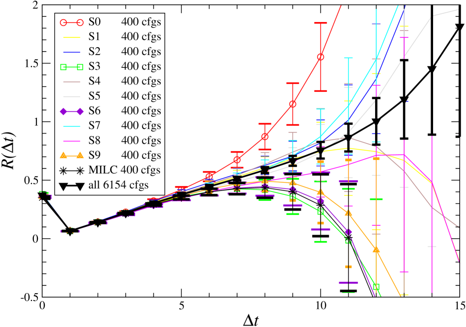
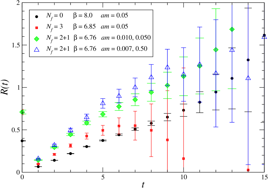
Figure 1: D/C ratio for 6154 $\beta=8.00$ quenched lattices with valence quark mass $am=0.05$, and for 11 subsets of 400 configurations. We highlight five of these subsets, including the original MILC configurations, as disagreeing with the mean by more than one $\sigma$.

Figure 2: $D/C$ ratio for coarse MILC ensembles. For the $N_{f}=3$ and $N_{f}=2+1$ ensembles $R_{SU3}$ is displayed. For the quenched configurations the single-flavour $R=D/C$ is plotted.

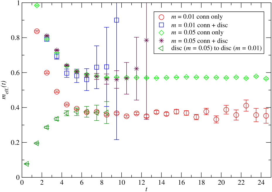
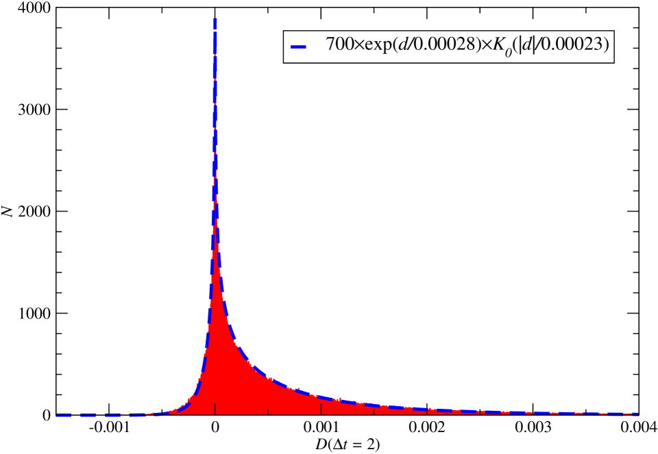
Figure 3: Effective masses for the $(\gamma_{5}\otimes{\bf 1})$ channel for the light and strange quarks for the $\beta$ = 6.76, m=0.01/0.05 data set.

Figure 4: Histogram of 393856 $D(\Delta t=2)$ measurements on 6154 quenched lattices.

5 Long dynamical ensemble

To attack the disconnected correlators forcefully, we have generated a $N_{f}=2+1$ flavor ensemble of 5081 configurations at intervals of six RHMC trajectories. These $24^{3}\times 64$ configurations with $\beta=6.75$ and $am=0.006,0.03$ have been generated on the UKQCD collaboration’s QCDOC machine. We chose the strange quark simulation mass of $am_{s}=0.03$ to coincide with values used by MILC in newer coarse ensembles [21].

$N_{f}$	$10/g^{2}$	$L^{3}\times T$	$am_{\rm sea}$	$am_{\rm val}$	$N_{\rm cfg}$
2+1	6.75	$24^{3}\times 64$	0.006, 0.030	00.006, 0.030	6000

Table 2: Long run dynamical ensembles for singlet calculations.

We have completed preliminary spectroscopy on a portion of this ensemble and find $aM_{\pi}=0.17478(35)$ and $aM_{\rho}=0.5298(17)$. A preliminary estimate of the static quark potential gives $r_{0}/a=3.810(51)$.

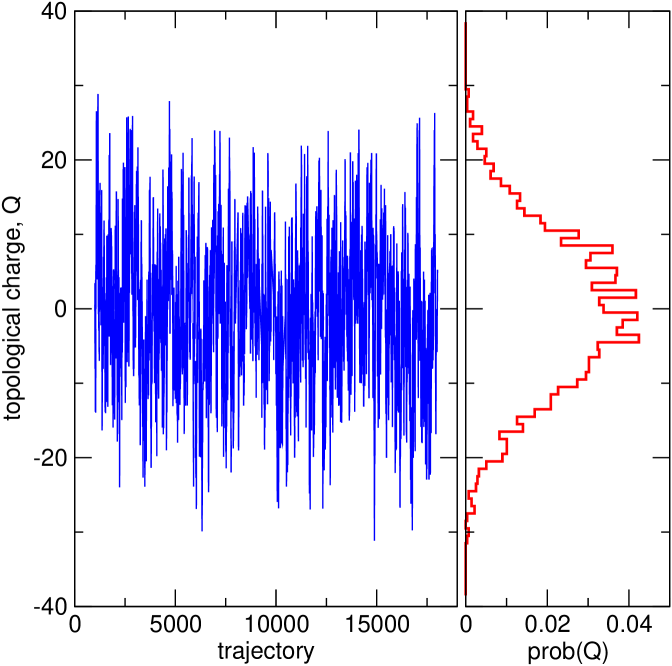
Figure 5: Topological charge time-series and histogram for about 17000 trajectories of the long dynamical run.

We have measured the topological charge on the ensemble and the time-history shows good tunnelling with an autocorrelation time in the range of 30 - 50 trajectories (Fig.5).

6 Conclusions and Outlook

We have completed the first phase of a project to explore singlet physics with staggered fermions. We have tested several methods of extracting singlet masses from connected and disconnected correlator combinations. We again refer the interested reader to the extended analysis in [13], including analysis of the other ensembles in Table 1.

Comparing the original and the extended quenched ensemble highlights the difficulties of working with “small” ensembles, and the need for long dynamical-fermion ensembles to calculate disconnected diagrams for singlet physics. We hope to be able to resolve the $\eta/\eta^{\prime}$ spectrum in the ensemble described in Section 5.

7 Acknowledgements

A portion of this analysis was performed on ScotGrid.

References

- [1] E. Witten, Nucl. Phys. B156, 269 (1979),
- [2] G. Veneziano, Nucl. Phys. B159, 213 (1979),
- [3] S. Itoh, Y. Iwasaki, and T. Yoshie, Phys. Rev. D36, 527 (1987),
- [4] UKQCD, C. McNeile and C. Michael, Phys. Lett. B491, 123 (2000), hep-lat/0006020,
- [5] TXL, T. Struckmann et al., Phys. Rev. D63, 074503 (2001), hep-lat/0010005,
- [6] CP-PACS, V. I. Lesk et al., Phys. Rev. D67, 074503 (2003), hep-lat/0211040,
- [7] K. Schilling, H. Neff, and T. Lippert, Lect. Notes Phys. 663, 147 (2005), hep-lat/0401005,
- [8] MILC, T. A. DeGrand and U. M. Heller, Phys. Rev. D65, 114501 (2002), hep-lat/0202001,
- [9] L. Venkataraman and G. Kilcup, (1997), hep-lat/9711006,
- [10] J. B. Kogut, J. F. Lagae, and D. K. Sinclair, Phys. Rev. D58, 054504 (1998), hep-lat/9801020,
- [11] H. Fukaya and T. Onogi, Phys. Rev. D70, 054508 (2004), hep-lat/0403024,
- [12] JLQCD, S. Aoki et al., (2006), hep-lat/0610021,
- [13] E. B. Gregory, A. C. Irving, C. M. Richards and C. McNeile, (2007) arXiv:0709.4224 [hep-lat].
- [14] HPQCD, C. T. H. Davies et al., Phys. Rev. Lett. 92, 022001 (2004), hep-lat/0304004,
- [15] C. Aubin et al., Phys. Rev. D70, 094505 (2004), hep-lat/0402030,
- [16] S. Durr, PoS LAT2005, 021 (2006), hep-lat/0509026,
- [17] S. R. Sharpe, PoS LAT2006, 022 (2006), hep-lat/0610094,
- [18] M. Creutz, Phys. Lett. B649, 230 (2007), hep-lat/0701018,
- [19] M. Creutz, (2007), arXiv:0708.1295 [hep-lat],
- [20] C. W. Bernard and M. F. L. Golterman, Phys. Rev. D46, 853 (1992), hep-lat/9204007,
- [21] C. Bernard et al. [MILC Collaboration], PoS LAT2005, 025 (2006) [arXiv:hep-lat/0509137].