Optimal Covariant Measurement of Momentum on a Half Line in Quantum Mechanics

Abstract

We cannot perform the projective measurement of a momentum on a half line since it is not an observable. Nevertheless, we would like to obtain some physical information of the momentum on a half line. We define an optimality for measurement as minimizing the variance between an inferred outcome of the measured system before a measuring process and a measurement outcome of the probe system after the measuring process, restricting our attention to the covariant measurement studied by Holevo. Extending the domain of the momentum operator on a half line by introducing a two dimensional Hilbert space to be tensored, we make it self-adjoint and explicitly construct a model Hamiltonian for the measured and probe systems. By taking the partial trace over the newly introduced Hilbert space, the optimal covariant positive operator valued measure (POVM) of a momentum on a half line is reproduced. We physically describe the measuring process to optimally evaluate the momentum of a particle on a half line.

I Introduction

Measurement in quantum mechanics is highly non-trivial as discussed in the mathematical foundation of quantum mechanics initiated by von Neumann neumann55 . He founded quantum mechanics on the Hilbert space and defined observables comment3 as self-adjoint operators to mathematically formulate the projection postulate in measuring processes by the spectral theory in functional analysis. Davies and Lewis constructed the framework of generalized measurement including the projective measurement by introducing the concept of the instrument and the positive operator valued measure (POVM) davies70 . Furthermore, by considering axioms of measuring devices, Ozawa introduced the completely positive (CP) instrument ozawa84 and showed that the state change by quantum measuring processes can be described in terms of the Kraus operators kraus71 and proposed a measuring apparatus, i.e., a scheme of measurement consisting of a probing process described only by quantum mechanics and a detection process described by the micro-macro coupling, which is to obtain classical information from quantum information  ozawa84 ; ozawa89 . To discuss measuring processes of the probe, we need to specify the Hilbert space corresponding to the probe system and an interaction Hamiltonian for the combined system of the measured system and the probe system to calculate an evolution operator. After the combined system is evolved in the measuring time, we acquire the measurement outcome of the probe system and obtain the state of the measured system after the measuring process taking the partial trace over the probe system. Note that we do not consider the detection process to obtain observational data corresponding to a macroscopic experimental result comment1 . All the above processes are summarized in the book busch91 , which is illustrated in Fig. 1.

For measuring processes, we shall consider an optimal measurement initiated by Helstrom helstrom74 . He defined an optimality of a measuring process to minimize the variance between an outcome of a measured system before the interaction and a measurement outcome of a probe system after the interaction. The optimal measurement sets upper limits to a POVM. In this paper, we explicitly construct a model Hamiltonian which reproduces the optimal POVM in a special case, while a general method is not available to construct a measurement model from a given POVM.

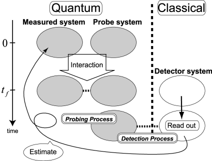
Figure 1: Scheme of measuring processes. We switch on the interaction between the measured and probe systems in the first step to obtain the measurement outcome of the probe system in the second step. We infer the observable of the measured system at $t=0$ from the outcome of the probe system at $t=t_{f}$ in the third step.

Let us recall that observables are defined as self-adjoint operators comment2 . In a general case of symmetric operators, we cannot apply the projection postulate since symmetric operators cannot generally be decomposed to real spectra, so that we have to consider generalized measurement davies70 . As an arch-typical example, we consider a half line system in quantum mechanics in this paper. In a half line system, a momentum is not an observable as will be seen in Sec. II. Here, our present proposal is to explicitly describe a generalized measuring process to optimally measure a momentum on a half line.

This paper is organized as follows. In Sec. II, we recapitulate the well-known property of a momentum operator in quantum mechanics on a half line and will see that the momentum on a half line is not an observable. In Sec. III, we define a covariant measurement and an optimality to measuring processes and then reproduce the optimal covariant POVM introduced by Holevo holevo78 ; holevo79 ; holevo82 ; holevo01 . In Sec. IV, we present a model Hamiltonian for the combined system of the measured and probe systems. We calculate a POVM from the model Hamiltonian to reproduce the result corresponding to the optimal covariant POVM. Furthermore, we present a physical description of our proposed measuring process. In Sec. V, we investigate the optimal covariant measurement model of the momentum on a half line. To make the momentum operator on a half line self-adjoint, we effectively extend the domain of this operator to the one of a whole line by tensoring a two dimensional Hilbert space. We apply the optimal measurement model in Sec. IV to the extended system. Taking the partial trace over the extra Hilbert space, we obtain the optimal covariant measurement model on a half line. Section VI is devoted to the summary and discussion.

II Quantum Mechanics on a Half Line

According to the functional analysis, on which the mathematical foundation of quantum mechanics neumann55 is based, an operator $\hat{A}$ is symmetric if $\hat{A}=\hat{A}^{\dagger}$, where $\hat{A}^{\dagger}$ is the Hermite conjugate. Further, a symmetric operator $\hat{A}$ is self-adjoint if ${\cal D}(\hat{A})={\cal D}(\hat{A}^{\dagger})$, where ${\cal D}(\hat{A})$ is the domain of the operator $\hat{A}$. In quantum mechanics, the observables are defined as self-adjoint operators, which have real spectra akhiezer81 . Symmetric operators, however, do not necessarily have a real spectrum. We need to classify symmetric operators into self-adjoint operators, essentially self-adjoint operators, self-adjoint extendable operators and non-self-adjoint extendable operators comment2 (for the definitions, see the book akhiezer81 ). A criterion is known as the deficiency theorem (See Appendix B).

Let us specifically consider a quantum system on a half line ${\mathbb{R}}_{+}\equiv[0,\infty)$. There have been many works concerning this problem since the beginning of quantum mechanics rellich50 ; clark80 ; farhi90 , e.g., the singular potential case50 ; krall82 ; gordeyev97 ; fulop07 . Recently, Fülöp et al. have studied boundary effects fulop02 ; tsutsui03 ; fulop05 and Twamley and Milburn have discussed a quantum measurement model on a half line by changing the coordinate $x\in{\mathbb{R}}_{+}$ to $\log x\in{\mathbb{R}}$ twamley06 .

In the following consideration, we characterize the half line system as follows. Let us take a Hilbert space ${\cal H}_{+}\equiv{\cal L}^{2}({\mathbb{R}}_{+})$ and a momentum operator $\hat{p}_{+}$ in ${\cal H}_{+}$ defined by

$$\hat{p}_{+}\psi(x) =\frac{1}{i}\frac{d}{dx}\psi(x),$$

$${\cal D}({\hat{p}}_{+}) =\left\{\psi\in{\cal H}_{+};\psi(0)=0,\int^{\infty}_{0}\left|\frac{d}{dx}\psi(x)\right|^{2}dx<\infty\right\}$$ (1)

in analogy to the standard momentum operator on a whole line. Throughout this paper, we take the unit $\hbar=1$.

Then we can see that $\hat{p}_{+}$ is symmetric since

$$\langle{\phi}|{{\hat{p}}_{+}\psi}\rangle =\frac{1}{i}\int^{\infty}_{0}\overline{\phi(x)}\frac{d}{dx}\psi(x)dx$$

$$=\left[\frac{1}{i}\overline{\phi(x)}\psi(x)\right]^{\infty}_{0}-\frac{1}{i}\int^{\infty}_{0}\frac{d}{dx}\overline{\phi(x)}\psi(x)dx$$

$$=\int^{\infty}_{0}\overline{\frac{1}{i}\frac{d}{dx}\phi(x)}\psi(x)dx$$

$$=\langle{{\hat{p}}^{\dagger}_{+}\phi}|{\psi}\rangle,$$ (2)

$$\psi\in{\cal D}({\hat{p}}_{+})\qquad\phi\in{\cal D}({\hat{p}}^{\dagger}_{+}),$$ (3)

where ${\hat{p}}^{\dagger}_{+}=\frac{1}{i}\frac{d}{dx}$ with

$${\cal D}({\hat{p}}^{\dagger}_{+})=\left\{\psi\in{\cal H}_{+};\int^{\infty}_{0}\left|\frac{d}{dx}\psi(x)\right|^{2}dx<\infty\right\}.$$ (4)

Therefore we conclude that $(\hat{p}_{+},{\cal D}(\hat{p}_{+}))\varsubsetneq({\hat{p}}^{\dagger}_{+},{\cal D}({\hat{p}}^{\dagger}_{+}))$ since ${\cal D}({\hat{p}}_{+})\neq{\cal D}({\hat{p}}^{\dagger}_{+})$. So the momentum operator ${\hat{p}}_{+}$ on a half line is symmetric but not self-adjoint, i.e., not an observable.

III Review of Optimal Covariant Measurement

Let us consider a measuring process described by an interaction between a measured system and a probe system, the latter of which is the part of the measuring apparatus as a whole. To establish the relationship between the measured and probe systems, we consider the momentum space $\Omega={\mathbb{R}}$ and a projective unitary representation of the shift group of $\Omega$. Stone’s theorem tells us that the unitary representation is given by

$$p\to V_{p}=e^{-ip\hat{x}},$$ (5)

where $\hat{x}$ is the position operator.

Definition 1.

A POVM $M(dp)$ is covariant with respect to the representation $p\to V_{p}$ if

$$V_{p}^{\dagger}M(\Delta)V_{p}=M(\Delta_{-p}),\quad p\in\Omega$$ (6)

for any $\Delta\in\mathcal{A}(\Omega)$, where

$$\Delta_{p}=\{p^{\prime}|p^{\prime}=p+p^{\prime\prime},p^{\prime\prime}\in\Delta\}$$ (7)

is the image of the set $\Delta$ under the transformation $p$ and $\mathcal{A}(\Omega)$ is the Borel $\sigma$-field of $\Omega$.

The covariant POVM has the property in the following form by using the Born formula neumann55 ; holevo82 ,

$$\Pr\{\hat{p}\in\Delta_{p}\|\rho_{p+p^{\prime}_{0}}\} =\operatorname{Tr}\rho_{p+p^{\prime}_{0}}M(\Delta_{p})=\operatorname{Tr}V_{-p}\rho_{p^{\prime}_{0}}V_{-p}^{\dagger}M(\Delta_{p})=\operatorname{Tr}\rho_{p^{\prime}_{0}}V_{-p}^{\dagger}M(\Delta_{p})V_{-p}=\operatorname{Tr}\rho_{p^{\prime}_{0}}M(\Delta)$$

$$=\Pr\{\hat{p}\in\Delta\|\rho_{p^{\prime}_{0}}\}.$$ (8)

That is, when the measured system is arbitrarily shifted, the measurement outcome is shifted by the same amount. This idealized measurement is called a covariant measurement. Realistic measuring devices, however, satisfy this condition only locally as discussed by Hotta and Ozawa hotta04 .

By von Neumann’s spectral theorem, any Hilbert space ${\cal H}$ can be formally described as the direct integral of a Hilbert space ${\cal H}_{x}$,

$${\cal H}=\int\oplus{\cal H}_{x}dx,$$ (9)

so that any state vector $\psi\in{\cal H}$ is described by the vector-valued function $\psi=[\psi_{x}]$ with $\psi_{x}\in{\cal H}_{x}$ introducing a convenient notation $[\,\cdot\,]$ holevo78 ; holevo82 . There, a position operator $\hat{x}$ acts as multiplication operators

$$\hat{x}\psi=[x\psi_{x}]$$ (10)

in this notation. The same notation $[\,\cdot\,]$ is used for an operator-valued function. A kernel $[K(x,x^{\prime})]$, where $K(x,x^{\prime})$ is a mapping from ${\cal H}_{x^{\prime}}$ to ${\cal H}_{x}$ for all $x$ and $x^{\prime}$, defines an operator $\hat{K}$ on ${\cal H}$. We can write

$$\hat{K}\psi=\left[K(x,x^{\prime})\right][\psi_{x^{\prime}}]=\left[\int K(x,x^{\prime})\psi_{x^{\prime}}dx^{\prime}\right].$$ (11)

Equations (10) and (11) can be rephrased by the bracket notation as

$$\hat{x}|{\psi}\rangle =\int dx|{x}\rangle x\langle{x}|{\psi}\rangle,$$ (12)

$$\hat{K}|{\psi}\rangle =\int dx\int dx^{\prime}|{x}\rangle K(x,x^{\prime})\langle{x^{\prime}}|{\psi}\rangle,$$ (13)

respectively. Also we express the norm in ${\cal H}_{x}$ as $\|\,\cdot\,\|_{x}$.

We are now in a position to explicitly describe the covariant POVM as follows.

Theorem 1 (Holevo holevo78 ).

Any covariant POVM in ${\cal H}$ has the form

$$M(dp)=\left[K(x,x^{\prime})e^{i(x-x^{\prime})p}\frac{dp}{2\pi}\right],$$ (14)

where $[K(x,x^{\prime})]$ is a positive definite kernel satisfying $K(x,x)\equiv I_{x}$, the identity mapping from ${\cal H}_{x}$ to itself.

In the above discussion, we have assumed that system and probe observables are isometric to obtain (14) as the POVM. The proof of Theorem 1 is given in Appendix A.

Next we turn to a measuring process. First, we couple a measured system to a probe system. Second, the combined system is evolved in time. Finally, we measure the probe observable. The sequence of processes enables us to retrospectively evaluate the system observable at the starting time by the measurement outcome of the probe observable at the end time (See Fig. 1). So we define the optimal covariant measurement as an optimal evaluation of the system observable by the outcome of the probe observable.

Let us assume that $W(p-P)$ is a deviation function, which expresses the variance between the inferred ”measurement” outcome $p$ of the system momentum before the interaction and the measurement outcome $P$ of the probe momentum after the interaction, satisfying

$$W(p)=-\int e^{ipx}\tilde{W}(dx),$$ (15)

for an even finite measure $\tilde{W}(dx)$ on ${\mathbb{R}}$. Let us consider the condition to minimize the variance

$$R_{p}\{M\}=\int_{\Omega}W(p-P)\mu_{\rho}(dp),$$ (16)

where $\mu_{\rho}(dp)\equiv\operatorname{Tr}\rho M(dp)$ is the probability distribution for the pure state $\rho=|{\psi}\rangle\!\langle{\psi}|$. Because of covariance, we rewrite (16) as

$$R_{0}\{M\} =\int_{\Omega}W(p)\mu_{\rho_{0}}(dp)$$

$$=-\int\Phi_{\rho}(x)\tilde{W}(dx),$$ (17)

where

$$\Phi_{\rho}(x)\equiv\int_{\Omega}e^{ixp}\langle{\psi}|{M(dp)\psi}\rangle$$ (18)

is a characteristic function of $\mu_{\rho}(dp)$. We get from Eq. (14)

$$\Phi_{\rho}(x)=\int\langle{\psi_{\mu}}|{K(\mu,\mu-x)\psi_{\mu-x}}\rangle d\mu.$$ (19)

Since the integral converges by the Cauchy-Swartz inequality and the condition $K(x,x)=I_{x}$,

$${\rm Re}\Phi_{\rho}(x)\leq\Phi_{\ast}(x)\equiv\int\|\psi_{\mu}\|_{\mu}\|\psi_{\mu-x}\|_{\mu-x}d\mu,$$ (20)

so that

$$R_{0}\{M\} \geq-\int\int\|\psi_{\mu}\|_{\mu}\|\psi_{\mu-x}\|_{\mu-x}d\mu\tilde{W}(dx)$$

$$\equiv R_{0}\{M_{0}\},$$ (21)

where

$$M_{0}(dp)=\left[\frac{\psi_{x}\cdot\psi_{x^{\prime}}^{\dagger}}{\|\psi_{x}\|_{x}\|\psi_{x^{\prime}}\|_{x^{\prime}}}e^{i(x-x^{\prime})p}\frac{dp}{2\pi}\right],$$ (22)

by transforming $\mu-x$ to $x^{\prime}$. Note that Eq. (22) does not depend on the choice of the deviation function $W(p-P)$ because of the covariance. It is curious to point out that this POVM corresponds to the optimal POVM under the unbiased condition hayashi00 . In the case of the whole line system, the optimal covariant POVM (22) in the bracket notation expresses

$$M_{0}(dp)=\int_{{\mathbb{R}}}dx\int_{{\mathbb{R}}}dx^{\prime}|{x}\rangle e^{i(x-x^{\prime})p}\frac{dp}{2\pi}\langle{x^{\prime}}|,$$ (23)

noting that the normalized term $\frac{\psi_{x}\cdot\psi_{x^{\prime}}^{\dagger}}{\|\psi_{x}\|_{x}\|\psi_{x^{\prime}}\|_{x^{\prime}}}$ is the identity in the bracket notation. By using the Fourier transformation,

$$|{p}\rangle=\frac{1}{\sqrt{2\pi}}\int_{{\mathbb{R}}}dxe^{ipx}|{x}\rangle,$$ (24)

Eq. (23) is transformed to the following equation:

$$M_{0}(dp)=|{p}\rangle\!\langle{p}|dp,$$ (25)

to obtain the projective measurement of a momentum on a whole line. To summarize the above discussion, we obtain the optimal covariant POVM (22) to minimize the estimated variance between the system and probe observables holevo78 ; holevo79 . We emphasize that Eq. (22) remains valid even when we change the domain of $x$.

IV Optimal Measurement Model on a Whole Line

In the previous section, we have obtained the optimal covariant POVM. We are now going to explicitly construct a Hamiltonian for a measurement model to realize the POVM. While it is straightforward to calculate the POVM and the probability distribution of the system observable for a given Hamiltonian of a combined system, it is not to find a Hamiltonian from a given POVM. In the two dimensional case, there is a way to construct a model Hamiltonian from a given POVM nielsen00 . Once the Hamiltonian for the combined system is found, we can physically realize the given POVM in principle. In the infinite dimensional case, we heuristically explore the optimal covariant POVM for the momentum in measuring processes in the following way. In this section, we preparatively discuss measurement of the momentum of a particle on a whole line and then apply the results to that on a half line in the next section. To make our exposition shorter, we assume that the wave functions $\{\psi_{x}\}$ are normalized and the measure $\frac{dp}{2\pi}$ is omitted in Eq. (22). Then Eq. (22) is simply

$$M_{0}=\left[\psi_{x}\cdot\psi_{x^{\prime}}^{\dagger}e^{i(x-x^{\prime})p}\right].$$ (26)

Let us consider a model Hamiltonian,

$${\hat{{\cal H}}}_{com} =\frac{1}{2m}{\hat{p}}^{2}+\frac{1}{2M}{\hat{P}}^{2}+g\hat{P}\hat{x}\delta(t)+\frac{m\omega^{2}}{2}{\hat{x}}^{2}$$

$$\equiv\hat{\mathcal{H}}_{0}+g\hat{P}\hat{x}\delta(t),$$ (27)

where a pair $(\hat{x},\hat{p})$ are the position and the momentum operators of the measured system, a pair $(\hat{X},\hat{P})$ are those of the probe system and $\delta(t)$ is the Dirac $\delta$-function. This Hamiltonian is modeled from the following consideration. We take the potential of the measured system as a harmonic oscillator for simplicity and the probe system is assumed to be a free particle system. Furthermore, the interaction is assumed to be instantaneous with a coupling constant $g$. The interaction term $g\hat{x}\hat{P}\delta(t)$ is chosen by the following reasoning. Because of the covariance, i.e., the measurement value $\tilde{P}$ of the probe observable corresponds to the ”measurement” value $\tilde{p}$ of the system observable at a certain time, we are led to an interaction of the momentum $\hat{P}$ of the probe system. Since the exponents in the optimal covariant POVM (26) has a quadratic form, a possible interaction term is either $g\hat{x}\hat{P}$ or $g\hat{p}\hat{P}$. The latter is excluded because it does not influence the momentum of the measured system.

Furthermore, we assume that the measured system itself is weakly coupled to a bulk system at zero temperature. We consider the measuring process from the time $t=0-$ to $t=t_{f}$. Then the evolution operator $\hat{\it U}$ becomes

$$\hat{\it U} ={\rm T}\;\exp\left(-i\int^{t_{f}}_{0-}{\hat{{\cal H}}}_{com}dt\right)$$

$$={\rm T}\;\exp\left(-i\int^{t_{f}}_{\epsilon}{\hat{{\cal H}}}_{0}dt\right)\exp\left(-i\int^{\epsilon}_{-\epsilon}g\hat{P}\hat{x}\delta(t)dt\right)$$

$$={\rm T}\;\exp\left(-i\int^{t_{f}}_{\epsilon}{\hat{{\cal H}}}_{0}dt\right)\exp\left(-ig\hat{P}\hat{x}(0)\right),$$ (28)

where $\epsilon$ is an infinitesimal positive parameter and ${\rm T}$ stands for the time-ordered product.

We construct the Kraus operator$[{\hat{A}}_{xx^{\prime}}]$ from the evolution operator as follows. Given the initial probe state $|{\tilde{P}}\rangle$, an eigen state of the momentum $\hat{P}$ of the probe system, we see that

$${\hat{A}}_{xx^{\prime}} =\int\langle{P}|\langle{x}|\hat{\it U}|{x^{\prime}}\rangle|{\tilde{P}}\rangle dP$$

$$=\sum_{j}\langle{x}|{\rm T}\;\exp\left(-i\int^{t_{f}}_{\epsilon}{\hat{{\cal H}}}_{0}dt\right)|{j}\rangle{\psi^{\dagger}}_{x^{\prime},j}\exp\left(-ig\tilde{P}x(0)\right)$$

$$\to\psi_{x}\cdot\psi^{\dagger}_{x^{\prime}}\exp\left(-ig\tilde{P}x(0)\right)\ \textrm{as}\;t_{f}\to\infty,$$ (29)

where $|{P}\rangle$ is an eigen state of $\hat{P}$, $\psi_{x,j}$ is the wave function corresponding to the $j$-th energy eigen state $|{j}\rangle$ and $\psi=[\psi_{x}]$ is the ground state of the free Hamiltonian $\hat{{\cal H}}_{0}$. In the last line of (29), the ground state is picked up in the limit $t_{f}\to\infty$. Physically speaking, we measure the probe observable after sufficient time passes. Recall that the standard i$\epsilon$ prescription abers73 implicitly assumes that the measured system itself is weakly coupled to the bulk system at zero temperature. Equation (29) is the matrix element of the Kraus operator $[{\hat{A}}_{xx^{\prime}}]$.

From the Kraus operator, we calculate the POVM as

$$M =\left[\int{\hat{A}}^{\dagger}_{x^{\prime}x^{\prime\prime}}{\hat{A}}_{xx^{\prime\prime}}dx^{\prime\prime}\right]$$ (30)

$$=\left[\psi^{\dagger}_{x^{\prime}}\cdot\psi_{x}\exp\left(-ig\tilde{P}\{x(0)-x^{\prime}(0)\}\right)\right].$$ (31)

We identify $g\tilde{P}$ with the measurement outcome $P$ itself of the probe observable to reproduce the optimal covariant POVM (26).

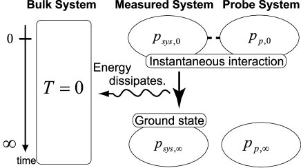
Figure 2: An optimal covariant measurement model. By the instantaneous interaction between the measured and probe systems, the measured system is entangled with the probe system. On the other hand, the measured system is coupled with the bulk system at zero temperature to dissipate the energy of the measured system. Thus we optimally evaluate the system observable at $t=0$ inferred from the outcome of the probe system at $t=\infty$ by the momentum conservation law.

Now, we physically describe how we optimally infer the momentum of the measured system just before the measuring process. First, we instantaneously couple the measured system to the probe system. Second, we keep the measured system in contact with the bulk system at zero temperature and wait for a sufficiently long time. Since the energy of the measured system is dissipated to the bulk system, the state of the measured system settles down to the ground state. If we let the energy of the ground state zero, i.e., $\omega\to 0$ of the interaction Hamiltonian (27), the momentum of the measured system $p_{sys,\infty}$ becomes zero at $t_{f}=\infty$. According to the momentum conservation law, we obtain

$$p_{sys,0}+p_{p,0}=p_{sys,\infty}+p_{p,\infty}=p_{p,\infty},$$ (32)

where $p_{sys,t}$ and $p_{p,t}$ are the momenta of the measured system and the probe system at a time $t$. Since we can control the probe system, we can precisely infer the ”measurement” value $p_{sys,0}$ of the momentum of the measured system at the beginning of the measuring process from the measurement outcome $p_{p,\infty}$, which we measure in the probe system at $t_{f}=\infty$ (See Fig. 2). If $\omega$ of the Hamiltonian (27) were finite, the variance of the momentum of the measured system would remain finite due to the zero point oscillation and Eq. (32) would be modified.

Although we have assumed that the potential of the measured system is given by the harmonic oscillator, the potential could actually be any convex function since the i$\epsilon$ prescription picks up the ground state at $t_{f}\to\infty$.

V Optimal Measurement Model on a Half Line

Let us apply the optimal measurement model to the half line system. We have already seen that the momentum operator (1) is not self-adjoint. First, we extend the domain of $\hat{p}_{+}$ á la Naimark so that the extended operator $\hat{p}$ is self-adjoint. The extended Hilbert space is

$${\cal H}={\cal H}_{+}\otimes{\cal H}_{2},$$ (33)

where ${\cal H}\equiv{\cal L}^{2}({\mathbb{R}})$, ${\cal H}_{+}\equiv{\cal L}^{2}({\mathbb{R}}_{+})$ and ${\cal H}_{2}$ is the two dimensional Hilbert space of the two level system with the orthonormal bases $|{0}\rangle$ and $|{1}\rangle$. We choose the form of the extended momentum operator as

$$\hat{p}=\hat{p}_{+}\otimes|{0}\rangle\!\langle{0}|-\hat{p}_{+}\otimes|{1}\rangle\!\langle{1}|.$$ (34)

By the unitary transformation $\Pi_{1}$, which is the space inversion around the zero point only for the spin state $|{1}\rangle$, the Hilbert space ${\cal H}$ is unitarily equivalent to

$${\cal H}={\cal H}_{+}\otimes|{0}\rangle+{\cal H}_{-}\otimes|{1}\rangle={\cal H}_{+}\oplus{\cal H}_{-},$$ (35)

where ${\cal H}_{-}\equiv{\cal L}^{2}({\mathbb{R}}_{-})$ and ${\mathbb{R}}_{-}\equiv(-\infty,0]$. Then we transform the extended momentum operator (34) by $\Pi_{1}$ as

$$\Pi_{1}\hat{p}\Pi^{\dagger}_{1}=\hat{p}_{+}\otimes|{0}\rangle\!\langle{0}|+\hat{p}_{-}\otimes|{1}\rangle\!\langle{1}|,$$ (36)

where $\hat{p}_{+}$ and $\hat{p}_{-}$ are momentum operators, which have the following domains

$${\cal D}(\hat{p}_{+}) =\left\{\psi\in{\cal H}_{+}\ ;\ \psi(0)=0,\int_{0}^{\infty}\left|\frac{d}{dx}\psi(x)\right|^{2}<\infty\right\}$$

$${\cal D}(\hat{p}_{-}) =\left\{\psi\in{\cal H}_{-}\ ;\ \psi(0)=0,\int_{-\infty}^{0}\left|\frac{d}{dx}\psi(x)\right|^{2}<\infty\right\},$$ (37)

respectively. Then the extended operator $\hat{p}$ is self-adjoint extendable since the domain is the Hilbert space for the whole line system. For a more precise argument, see Appendix B, where the choice of a boundary condition $\psi(0)=0$ is also justified. These operations are exhibited in Fig. 3. It is curious to point out that this operator $\hat{p}$ is $\cal{PT}$ symmetric noting that the spin states $|{0}\rangle$ and $|{1}\rangle$ are interchanged by the time reversal $\cal{T}$ and the momentum operators $\hat{p}_{+}$ and $\hat{p}_{-}$ by the parity inversion and the time reversal $\cal{PT}$. We can see that the spectrum of $\hat{p}$ is real also from this reasoning bender07 .

Figure 3: A Naimark extension. An auxiliary two dimensional Hilbert space ${\cal H}_{2}$ is tensored to the Hilbert space ${\cal H}_{+}$ to prepare the two (original and copied) Hilbert spaces. Then we spatially invert the copied Hilbert space around the zero point. Finally, we combine the original and inverted Hilbert spaces to obtain the extended Hilbert space, ${\cal H}={\cal H}_{+}\otimes{\cal H}_{2}={\cal H}_{+}\oplus{\cal H}_{-}$.

We adopt the form of the model Hamiltonian (27) with $\hat{p}$ being replaced by the right hand side of (36) and $x\in{\mathbb{R}}$, so that all the operators in the Hamiltonian (27) are self-adjoint to construct the optimal covariant measurement in the same way as described in Sec. IV. We, then, calculate the Kraus operator from the model Hamiltonian by using the i$\epsilon$ prescription. Since we have chosen $\psi(0)=0$, we end up with the ground state with odd parity with the energy $\frac{3}{2}\omega$. The Kraus operator is then

$$\Pi_{1}[{\hat{A}}_{xx^{\prime}}]\Pi^{\dagger}_{1}=\left[\psi_{x_{+}}\cdot\psi^{\dagger}_{x^{\prime}_{+}}\exp\left(-igP_{+}x_{+}(0)\right)\right]\otimes|{0}\rangle\!\langle{0}|+\left[\psi_{x_{-}}\cdot\psi^{\dagger}_{x^{\prime}_{-}}\exp\left(-igP_{-}x_{-}(0)\right)\right]\otimes|{1}\rangle\!\langle{1}|.$$ (38)

From Eq. (30), the Kraus operator (38) gives the following POVM,

$$\Pi_{1}M_{0}\Pi^{\dagger}_{1}=\left[\psi_{x_{+}}\cdot\psi_{x^{\prime}_{+}}^{\dagger}e^{i(x_{+}-x^{\prime}_{+})p_{+}}\right]\otimes|{0}\rangle\!\langle{0}|+\left[\psi_{x_{-}}\cdot\psi_{x^{\prime}_{-}}^{\dagger}e^{i(x_{-}-x^{\prime}_{-})p_{-}}\right]\otimes|{1}\rangle\!\langle{1}|.$$ (39)

By taking the partial trace over ${\cal H}_{2}$, we obtain the reduced POVM

$${\tilde{M}}_{0} \equiv\operatorname{Tr}_{2}M_{0}$$

$$=\left[\psi_{x_{+}}\cdot\psi^{\dagger}_{{x^{\prime}_{+}}}e^{i(x_{+}-x^{\prime}_{+})p_{+}}\right],$$ (40)

up to a normalization constant. Here in Eq. (40), we have transformed (39) back to $M_{0}$ by the unitary operator $\Pi_{1}$ and reproduced the optimal covariant POVM (26) restricted to positive parameters $x$ and $x^{\prime}$.

Finally, we calculate the probability distribution of the momentum on a half line in the optimal case. As an example, let us assume the pure state $\rho=\left[\phi_{x_{+}}\cdot\phi^{\dagger}_{x^{\prime}_{+}}\right]$, which is a plane wave with a momentum $p_{true}$,

$$\phi_{x_{+}}=Ae^{ip_{true}x_{+}},$$ (41)

for the measured system before the measuring process. We assume that the state (41) is properly localized to be an element of the Hilbert space ${\cal H}_{+}$. The state (41), $\left[\phi_{x_{+}}\right]$, is relaxed by the measuring process to the ground state $\psi_{x_{+}}\in{\cal H}_{+}$ given by

$$\psi_{x_{+}}=2\left(\frac{(m\omega)^{3}}{\pi}\right)^{\frac{1}{4}}x_{+}\exp\left(-\frac{m\omega}{2}x^{2}_{+}\right).$$ (42)

Then we obtain the probability distribution of the momentum as

$$\operatorname{Tr}(\rho{\tilde{M}}_{0}) =\operatorname{Tr}\left(\left[\phi_{x^{\prime\prime}_{+}}\cdot\phi^{\dagger}_{x^{\prime}_{+}}\right]\left[\psi_{x_{+}}\cdot\psi^{\dagger}_{{x^{\prime\prime}_{+}}}e^{i(x_{+}-x^{\prime\prime}_{+})p}\right]\right)$$

$$=\int\int\phi_{x^{\prime\prime}_{+}}\cdot\phi^{\dagger}_{x_{+}}\cdot\psi_{x_{+}}\cdot\psi^{\dagger}_{{x^{\prime\prime}_{+}}}e^{i(x_{+}-x^{\prime\prime}_{+})p}dxdx^{\prime\prime}$$

$$=16\sqrt{\frac{\pi}{(m\omega)^{3}}}|A|^{2}\left(p-p_{true}\right)^{2}\exp\left(-\frac{1}{m\omega}\left(p-p_{true}\right)^{2}\right),$$ (43)

which has two peaks at $p=p_{true}\pm\sqrt{m\omega}$ and vanishes at $p=p_{true}$. If we take $\omega\to 0$, i.e., the measured system is a free particle system, we can precisely evaluate the momentum of the plane wave since we obtain $\operatorname{Tr}(\rho{\tilde{M}}_{0})=\delta(p-p_{true})$. Otherwise there remains uncertainty by quantum zero point oscillation and the momentum with the maximum probability deviates by $\sqrt{m\omega}$ from the precise momentum $p_{true}$. When the potential of the measured system is a general convex function, the probability distribution for the momentum becomes the modulus square of the Fourier transformation of the odd parity ground state wave function.

To summarize this section, we have obtained the optimal covariant POVM on a half line, which enables us to explicitly construct the measuring process of the momentum on a half line.

VI Summary and Discussion

We have considered the optimal covariant measurement of momenta on a half line. Since the momentum operator $\hat{p}_{+}=\frac{1}{i}\frac{d}{dx}$ on a half line is not self-adjoint, i.e., not an observable. By applying the Naimark extension, the measured system is extended to the whole line and the momentum operator on the extended system becomes self-adjoint. Then we have discussed the optimal covariant measurement model on the extended system. By applying Holevo’s works holevo78 ; holevo79 ; holevo82 ; holevo01 , we have obtained the optimal covariant POVM in the optimal sense to minimize the variance between the ”measurement” outcome of the measured system before the interaction and the measurement outcome of the probe system after the interaction. To realize physical systems, we have explicitly constructed the model Hamiltonian for the measured and probe systems and coupled the measured system to the bulk system at zero temperature for infinitely long time. We have shown that the optimal covariant POVM coincides with the calculated POVM from the model Hamiltonian. As a result, we have presented the optimal covariant measurement model. Then we have physically explained the optimal covariant measuring process. By taking the partial trace over the auxiliary Hilbert space ${\cal H}_{2}$, we have described the optimal covariant measurement model for the momentum on a half line and calculated the optimal probability distribution of the momentum on a half line in a special case.

The following points remain to be clarified. First, we have only discussed the covariant case. Peres and Scudo, however, pointed out that the covariant measurement may not be optimal and mentioned counterexamples in quantum phase measurement peres02 . We have to check whether the optimality for any measurement is the optimal covariant measurement in our setup or not. Second, Ozawa have recently constructed a new Heisenberg uncertainty principle ozawa03 ; ozawa04 . The inequality expresses a quantum limit of measuring processes. It will be interesting to examine Ozawa’s inequality in our framework. Third, there is an analogy between a momentum operator on a half line and a time or time-of-arrival operator since a energy has a lower bound. However, there has been a long debate about mathematical formulations and physical meanings of a time or time-of-arrival operator (for example holevo82 ; aharonov61 ; baute00 ; arai08 ). It will be interesting to show physical meanings of this operator motivated by our framework. Finally, we have presented the model Hamiltonian (27) to physically realize the optimal covariant POVM (22). We do not know a general method to construct a Hamiltonian from an arbitrary POVM. Our analysis may be a clue to the general method to solve the inverse problem. Furthermore, to experimentally demonstrate the measurement model, experimental setups remain to be considered for our proposed model Hamiltonian.

Appendix A Proof of Theorem 1

A measure $\nu$ is called invariant on $\mathcal{A}(\Omega)$ if and only if for any $p\in\Omega$ there exists a measure $\nu$ such that

$$\nu(\Delta_{p})=\nu(\Delta),$$ (44)

where $\Delta$ is an element of $\mathcal{A}(\Omega)$ and $\Delta_{p}$ is defined in (7).

The following lemma is useful.

Lemma 1.

Let $M(dp)$ be a covariant POVM with respect to a projective unitary representation $p\to V_{p}$ of the parametric group $G$ of transformations of the set $\Omega$. For any density operator $\rho$ on the Hilbert space of the representation and for any Borel set $\Delta\in\mathcal{A}(\Omega)$

$$\int_{\Omega}\operatorname{Tr}V_{p}\rho V^{\dagger}_{p}M(\Delta)\mu(dp)=\nu(\Delta)$$ (45)

where $\mu(dp)$ is the proper Lebesgue measure and the extent $\Omega$ of the integral is a space of parameters in $G$ and $\nu$ is an invariant measure.

Proof.

Define

$$\mathbf{1}_{\Delta}(p)=\biggl{\{}\begin{array}[]{ll}1&\textrm{on}\;p\in\Delta\\ 0&\textrm{on}\;p\notin\Delta\end{array}.$$ (46)

Then we can write the left hand side of (45) as

$$\int_{\Omega}\operatorname{Tr}V_{p}\rho V^{\dagger}_{p}M(\Delta)\mu(dp)=\int_{\Omega}\operatorname{Tr}\rho M(\Delta_{-p})\mu(dp)=\int_{\Omega}\int_{\Omega}\mathbf{1}_{\Delta}(p+p_{0})\mu_{\rho}(dp_{0})\mu(dp),$$ (47)

where $\mu_{\rho}(dp_{0})\equiv\operatorname{Tr}\rho M(dp_{0})$ is the probability distribution of the momentum for the state $\rho$ noting that the second integral on the rightmost side is over the whole momentum space $\Omega$. We see that

$$\int_{\Omega}\mu_{\rho}(dp_{0})\int_{\Omega}\mathbf{1}_{\Delta}(p+p_{0})\mu(dp)=\nu(\Delta).$$ (48)

The following is the proof of Theorem 1.

Proof.

Let us assume $\rho=|{\psi}\rangle\langle{\psi}|$ without loss of generality. Then we see that

$$\int_{\Omega}V_{p}\rho V^{\dagger}_{p}\frac{dp}{2\pi}=\left[\int_{\Omega}e^{ipx}\psi_{x}\cdot\psi^{\dagger}_{x^{\prime}}e^{-ipx^{\prime}}\frac{dp}{2\pi}\right]=\left[\delta(x-x^{\prime})\psi_{x}\cdot\psi^{\dagger}_{x}\right].$$ (49)

Noting that the operator $M(\Delta)$ is defined by the kernel $M_{\Delta}(x,x^{\prime})$, we obtain from Lemma 1 and Eq. (49)

$$\int_{G}\psi^{\dagger}_{x}M_{\Delta}(x,x)\psi_{x}dx=\frac{\mathrm{mes}\Delta}{2\pi},$$ (50)

where $G$ is the parametric group and $\mathrm{mes}\Delta$ denotes the Lebesgue measure of $\Delta$. Since $[\psi_{x}]$ is arbitrary, we see that $M_{\Delta}(x,x)=\frac{1}{2\pi}\mathrm{mes}\Delta\cdot I_{x}$ noting that $I_{x}$ is the identity mapping from ${\cal H}_{x}$ to itself. From the positive definiteness of $M_{\Delta}(x,x^{\prime})$, we can derive that

$$|\psi^{\dagger}_{x}M_{\Delta}(x,x^{\prime})\psi_{x^{\prime}}|\leq\sqrt{\psi^{\dagger}_{x}M_{\Delta}(x,x)\psi_{x}}\sqrt{\psi^{\dagger}_{x^{\prime}}M_{\Delta}(x^{\prime},x^{\prime})\psi_{x^{\prime}}}=\|\psi_{x}\|_{x}\|\psi_{x^{\prime}}\|_{x^{\prime}}\frac{\mathrm{mes}\Delta}{2\pi}$$ (51)

using the Cauchy-Schwartz inequality. Therefore, the measure $M_{\Delta}(x,x^{\prime})$ is absolutely continuous with respect to the Lebesgue measure, so that we can express

$$M_{\Delta}(x,x^{\prime})=\frac{1}{2\pi}\int_{\Delta}K_{p}(x,x^{\prime})dp,$$ (52)

with $K_{p}(x,x^{\prime})$ being some positive definite density satisfying $K_{p}(x,x)=I_{x}$. From the covariance properties, it follows that

$$K_{p}(x,x^{\prime})=e^{i(x-x^{\prime})p}K_{0}(x,x^{\prime}).$$ (53)

Putting $K_{0}(x,x^{\prime})=K(x,x^{\prime})$, we get (14) in Theorem 1.

Appendix B Deficiency Theorem

We refer the reader to the book reed75 and the paper bonneau01 for details. We shall give a criterion for closed symmetric operators to be self-adjoint operators.

Let us assume that $(\hat{A},{\cal D}(\hat{A}))$ is densely defined, symmetric and closed. One defines the deficiency subspaces ${\cal N}_{\pm}$ by, for a fixed $\gamma>0$,

$${\cal N}_{+}=\{\psi\in{\cal D}(\hat{A}^{\dagger})\,;\ \hat{A}^{\dagger}\psi=i\gamma\psi\}$$ (54)

$${\cal N}_{-}=\{\psi\in{\cal D}(\hat{A}^{\dagger})\,;\ \hat{A}^{\dagger}\psi=-i\gamma\psi\}$$ (55)

of respective dimensions $n_{+}$ and $n_{-}$, which are called the deficiency indices of the operator $\hat{A}$ and denoted by a pair $(n_{+},n_{-})$. The following theorem holds.

Theorem 2 (Deficiency theorem).

For any closed symmetric operator $\hat{A}$ with deficiency indices $(n_{+},n_{-})$, there are three possibilities:

1. $\hat{A}$ is self-adjoint if and only if $n_{+}=n_{-}=0$.

2. $\hat{A}$ has self-adjoint extensions if and only if $n_{+}=n_{-}$. There exists one-to-one correspondence between self-adjoint extension of $\hat{A}$ and unitary maps from ${\cal N}_{+}$ to ${\cal N}_{-}$.

3. If $n_{+}\neq n_{-}$, $\hat{A}$ has no self-adjoint extension.

This theorem is firstly discussed by Weyl weyl10 and generalized by von Neumann neumann29 .

Let us apply this theorem to the momentum operator (1) on a half line. First, we solve the differential equations,

$$\hat{p}_{+}\psi_{\pm}(x)=-i\frac{d}{dx}\psi_{\pm}(x)=\pm i\gamma\psi_{\pm}(x),$$ (56)

where $\gamma$ is real and positive to obtain

$$\psi_{\pm}(x)\sim e^{\mp\gamma x}.$$ (57)

Because of $\psi\in{\cal L}^{2}({\mathbb{R}}_{+})$, only $\psi_{+}(x)$ is allowed. Therefore, we obtain the deficiency indices $(1,0)$ and conclude, by the deficiency theorem, $\hat{p}_{+}$ has no self-adjoint extension.

As another example, we show that the extended momentum operator (34) is self-adjoint extendable. We obtain the deficiency indices $(0,1)$ of $-\hat{p}_{+}$ in the same way. So the deficiency indices of the extended momentum operator (34) are $(1,1)$ and the operator is self-adjoint extendable by the deficiency theorem. Since the self-adjoint extension is parametrized by $U(1)$, $\psi(0+)=e^{i\theta}\psi(0-)$ where $\theta\in{\mathbb{R}}$, we have a freedom to choose the boundary conditions at the origin by that amount. The boundary condition $\psi(0)=0$ chosen in the main text, which comes from the physical requirement to the half line system, is mathematically legitimate in the extended system because it is a special case of the $U(1)$ variety.

References

- (1) J. von Neumann, Mathematische Grundlagen der Quantumechanik (Springer, Berlin, 1932), [ Mathematical foundations of quantum mechanics (Princeton University Press, Princeton, 1955). ]
- (2) The ”observable” is a technical term. We use this term as a self-adjoint operator á la von Neumann by the Kato-Rellich theorem while the use of this term might be controversial.
- (3) E. B. Davies and J. T. Lewis, Commun. Math. Phys. 17, 239-260 (1970).
- (4) M. Ozawa, J. Math. Phys. 25, 79-87 (1984).
- (5) K. Kraus, Ann. Phys. 64, 311-335 (1971).
- (6) M. Ozawa, in Squeezed and Nonclassical Light, edited by P. Tombesi and E. R. Pike, (Plenum, New York, 1989), pp. 263- 286.
- (7) We often call the detection process a magnification process, which is how to observe a pointed value of measuring devices, e.g., physical processes in a photomultiplier. This process is discussed by many people, e.g., see Ojima ojima07 .
- (8) P. Busch, P. Mittelstaedt and P. J. Lahti, Quantum Theory of Measurement (Springer-Verlag, Berlin, 1991).
- (9) C. W. Helstrom, Int. J. Theor. Phys. 11, 357-378 (1974).
- (10) Many physicists do not classify symmetric operators into self-adjoint operators and often call a symmetric operator Hermitian and identify a Hermitian operator with an observable without checking a domain of a operator (See, e.g., schiff65 ; landau77 ).
- (11) A. S. Holevo, Rep. Math. Phys. 13, 379-399 (1978).
- (12) A. S. Holevo, Rep. Math. Phys. 16, 385-400 (1979).
- (13) A. S. Holevo, Probabilistic and statistical aspects of quantum theory (North-Holland, Amsterdam, 1982).
- (14) A. S. Holevo, Statistical Structure of Quantum Theory (Springer, Berlin, 2001).
- (15) N. I. Akhiezer and I. M. Glazman, Theory of Linear Operators in Hilbert Space (Dover, New York, 1993).
- (16) F. Rellich, Math. Ann. 122, 343-368 (1950).
- (17) T. E. Clark, R. Menioff and D. H. Sharp, Phys. Rev. D 22, 3012-3016 (1980).
- (18) E. Farhi and S. Gutmann, Int. J. Mod. Phys. A 5, 3029-3051 (1990).
- (19) K. M. Case, Phys. Rev. 80, 797-806 (1950).
- (20) A. M. Krall, J. Diff. Eq. 45, 128-138 (1982).
- (21) A. N. Gordeyev and S. C. Chhajlany, J. Phys. A 30, 6893-6909 (1997).
- (22) T. Fülöp, arXiv:0708.0866.
- (23) T. Fülöp, T. Cheon and I. Tsutsui, Phys. Rev. A 66, 052102 (2002).
- (24) I. Tsutsui, T. Fülöp and T. Cheon, J. Phys. A 36, 275-287 (2003).
- (25) T. Fülöp, Ph.D. thesis, University of Tokyo, 2005.
- (26) J. Twamley and G. J. Milburn, New J. of Phys. 8, 328 (2006).
- (27) M. Hotta and M. Ozawa, Phys. Rev. A 70, 022327 (2004).
- (28) M. Hayashi and F. Sakaguchi, J. Phys. A 33, 7793 (2000).
- (29) M. A. Nielsen and I. L. Chuang, Quantum Computation and Quantum Information (Cambridge University Press, Cambridge, 2000).
- (30) E. S. Abers and B. W. Lee, Phys. Rep. 9, 1-141 (1973).
- (31) C. M. Bender, Rep. Prog. Phys. 70, 947-1018 (2007).
- (32) A. Peres and P. Scudo, J. Mod. Opt. 49, 1235-1243 (2002).
- (33) M. Ozawa, Phys. Rev. A 67, 042105 (2003).
- (34) M. Ozawa, Ann. Phys. 311, 350-416 (2004).
- (35) Y. Aharonov and D. Bohm, Phys. Rev. 122, 1649 (1961).
- (36) A. D. Baute, I. L. Egusquiza, J. G. Muga and R. Sala Mayato, Phys. Rev. A 61, 052111 (2000).
- (37) A. Arai and Y. Matsuzawa, mp-arc:08-24 (2008).
- (38) M. Reed and B. Simon, Methods of Modern Mathematical Physics II, Fourier Analysis, Self-Adjointness (Academic Press, New York, 1975).
- (39) G. Bonneau, J. Faraut and G. Valent, Am. J. Phys. 69, 322-331 (2001).
- (40) H. Weyl, Math. Ann. 68, 220-269 (1910).
- (41) J. von Neumann, Math. Ann. 102, 49-131 (1929).
- (42) I. Ojima, arXiv:0705.2945.
- (43) L. I. Schiff, Quantum Mechanics (McGraw-Hill, 1965) Third edition.
- (44) L. D. Landau and E. M. Lifschitz, Quantum Mechanics Non-Relativistic Theory (Pergamon Press, 1977) Third edition.