Trading activity as driven Poisson process: comparison with empirical data

Abstract

We propose the point process model as the Poissonian-like stochastic sequence with slowly diffusing mean rate and adjust the parameters of the model to the empirical data of trading activity for 26 stocks traded on NYSE. The proposed scaled stochastic differential equation provides the universal description of the trading activities with the same parameters applicable for all stocks.

, url]http://www.itpa.lt/ gontis ,

1 Introduction

A possible way to avoid the inconsistence of geometric Brownian motion as a model of speculative markets is the assumption that the volatility is itself a time-depending random variable. Within this assumption there exist the discrete ARCH and GARCH models [1, 2, 3, 4] as well as the continuous stochastic volatility models [5, 6, 7]. It is empirically established that the autocorrelation function of volatility decays very slowly with time exhibiting two different exponents of the power-law distribution: for short time scales and for the long time ones. However, common stochastic volatility models are able reproduce only one time scale exponential decay [6, 8]. There is empirical evidence that the trading activity is a stochastic variable with the power-law probability distribution function (PDF) [9, 10] and the long-range correlations [4, 11, 12] resembling the power-law statistical properties of volatility. Empirical analysis confirms that the long-range correlations in volatility arise due to those of the trading activity [11]. On the other hand, the trading activity can be modeled as the event flow of the stochastic point process with more evident microscopic interpretation of the observed power-law statistics.

Recently, we proposed the stochastic model of the trading activity in the financial markets as Poissonian-like process driven by the stochastic differential equation (SDE) [13, 14]. Here we present the detailed comparison of the model with the empirical data of the trading activity for 26 stocks traded on NYSE. This enables us to present a more precise model definition based on the scaled equation, universal for all stocks. The proposed form of the difference equation for the intertrade time can be interpreted as a discrete iterative description of the proposed model, based on SDE.

2 Stochastic model of trading activity

We consider trades in the financial market as identical point events. Such point process is stochastic and defined by the stochastic interevent time $\tau_{k}=t_{k+1}-t_{k}$, with $t_{k}$ being the occurrence times of the events. Recently we proposed [13, 14] to model the flow of trades in the financial markets as Poissonian-like process driven by the multiplicative stochastic equation, i.e. we define the rate $n=1/\tau$ of this process by the continuous stochastic differential equation

$$\mathrm{d}n=\sigma^{2}\left[(1-\gamma_{\sigma})+\frac{m}{2}\left(\frac{n_{0}}{n}\right)^{m}\right]\frac{n^{4}}{(n\epsilon+1)^{2}}\mathrm{d}t+\frac{\sigma n^{5/2}}{(n\epsilon+1)}\mathrm{d}W.$$ (1)

This SDE with the Wiener noise $W$ describes the diffusion of the stochastic rate $n$ restricted in some area: from the side of the low values by the term $m(n_{0}/n)^{m}/2$ and from the side of high values by the relaxation $\gamma_{\sigma}$. The general relaxation factor $\sigma^{2}n^{4}/(n\epsilon+1)^{2}\mathrm{d}t$ is keyed with multiplicative noise $\sigma n^{5/2}/(n\epsilon+1)\mathrm{d}W$ to ensure the power-law distribution of $n$. The multiplicative noise is combined of two powers to ensure the spectral density of $n$ with two power law exponents. This form of the multiplicative noise helps us to model the empirical probability distribution of the trading activity, as well. A parameter $\epsilon$ defines the crossover between two areas of $n$ diffusion. For more details see [13, 14]. Equation (1) has to model stochastic rate $n$ with two power-law statistics, i.e., PDF and power spectral density or autocorrelation, resembling the empirical data of the trading activity in the financial markets.

We will analyze the statistical properties of the trading activity $N(t,\tau_{\mathrm{d}})$ defined as integral of $n$ in the selected time window $\tau_{\mathrm{d}}$,

$$N(t,\tau_{\mathrm{d}})=\int_{t}^{t+\tau_{\mathrm{d}}}n(t^{\prime})\mathrm{d}t^{\prime}.$$ (2)

The Poissonian-like sequence of trades described by the intertrade times $\tau_{k}$ can be generated by the conditional probability

$$\varphi(\tau_{k}|n)=n\exp(-n\tau_{k}).$$ (3)

In the case of single exponent power law model, see [13, 14], when PDF of $n$ is $P(n)\sim n^{-\lambda}\exp\{-(n_{\mathrm{0}}/n)^{m}\}$, the distribution $P(\tau_{k})$ of intertrade time $\tau_{k}$ in $k$-space has the integral form

$$P(\tau_{k})=C\int_{0}^{\infty}\exp(-n\tau_{k})n^{1-\lambda}\exp\left[-\left(\frac{n_{0}}{n}\right)^{m}\right]\mathrm{d}n,$$ (4)

with $C$ defined from the normalization, $\int_{0}^{\infty}P(\tau_{k})\mathrm{d}\tau_{k}=1$. The explicit expressions of the integral (4) are available for the integer values of $m$. When $m=1$, PDF (4) is expressed through the Bessel function of the second kind whereas for $m>1$ the more complicated structures of distribution $P(\tau_{k})$ expressed in terms of hypergeometric functions arise.

Now we have the complete set of equations defining the stochastic model of the trading activity in the financial markets. We proposed this model following our increasing interest in the stochastic fractal point processes [15, 16, 17, 18]. Our objective to reproduce in details statistics of trading activity conditions rather complicated form of the SDE (1) and low expectation of analytical results. In this paper we focus on the numerical analysis and direct comparison of the model with the empirical data. In order to achieve more general description of statistics for different stocks we introduce the scaling to Eq. (1) with scaled time $t_{s}=\sigma^{2}n_{0}^{3}t$, scaled rate $x=n/n_{0}$ and $\varepsilon^{\prime}=\varepsilon n_{0}$. Then Eq. (1) becomes

$$\mathrm{d}x=\left[(1-\gamma_{\sigma})+\frac{m}{2}x^{-m}\right]\frac{x^{4}}{(x\varepsilon^{\prime}+1)^{2}}+\frac{x^{5/2}}{(x\varepsilon^{\prime}+1)}\mathrm{d}W_{s}.$$ (5)

The parameter $n_{0}$ specific for various stocks is now excluded from the SDE and we have only three parameters to define from the empirical data of trading activity in the financial markets. We solve Eq. (5) using the method of discretization. Introducing the variable step of integration $\Delta t_{s}=h_{k}=\kappa^{2}/x_{k}$, the differential equation (5) transforms to the difference equation

$$x_{k+1} = x_{k}+\kappa^{2}\left[(1-\gamma_{\sigma})+\frac{m}{2}x_{k}^{-m}\right]\frac{x_{k}^{3}}{(x_{k}\epsilon^{\prime}+1)^{2}}+\kappa\frac{x_{k}^{2}}{(x_{k}\epsilon^{\prime}+1)}\varepsilon_{k},$$ (6)

$$t_{k+1} = t_{k}+\kappa^{2}/x_{k}$$ (7)

with $\kappa\ll 1$ being a small parameter and $\varepsilon_{k}$ defining Gaussian noise with zero mean and unit variance .

With the change of variables $\tau=1/n$ one can transform Eq. (1) into

$$\mathrm{d}\tau=\sigma^{2}\left[\gamma_{\sigma}-\frac{m}{2}\left(\frac{\tau}{\tau_{0}}\right)^{m}\right]\frac{1}{(\epsilon+\tau)^{2}}dt+\sigma\frac{\sqrt{\tau}}{\epsilon+\tau}\mathrm{d}W$$ (8)

with limiting time $\tau_{0}=1/n_{0}$. We will show that this form of driving SDE is more suitable for the numerical analysis. First of all, the powers of variables in this equation are lower and the main advantage is that the Poissonian-like process can be included into the procedure of numerical solution of SDE. We introduce a scaling of Eq. (8) with the nondimensional scaled time $t_{s}=t/\tau_{0}$, scaled intertrade time $y=\tau/\tau_{0}$ and $\epsilon^{\prime}=\epsilon/\tau_{0}$. Then Eq. (8) becomes

$$\mathrm{d}y=\frac{\sigma^{2}}{\tau_{0}^{2}}\left[\gamma_{\sigma}-\frac{m}{2}y^{m}\right]\frac{1}{(\epsilon^{\prime}+y)^{2}}\mathrm{d}t_{s}+\frac{\sigma}{\tau_{0}}\frac{\sqrt{y}}{\epsilon^{\prime}+y}\mathrm{d}W_{s}.$$ (9)

As in the real discrete market trading we can choose the instantaneous intertrade time $y_{k}$ as a step of numerical calculations, $h_{k}=y_{k}$, or even more precisely as the random variables with the exponential distribution $P(h_{k})=1/y_{k}\exp(-h_{k}/y_{k})$. Then we get the iterative equation resembling tick by tick trades in the financial markets,

$$y_{k+1}=y_{k}+\frac{\sigma^{2}}{\tau_{0}^{2}}\left[\gamma_{\sigma}-\frac{m}{2}y_{k}^{m}\right]\frac{h_{k}}{(\epsilon^{\prime}+y_{k})^{2}}+\frac{\sigma}{\tau_{0}}\frac{\sqrt{y_{k}h_{k}}}{\epsilon^{\prime}+y_{k}}\varepsilon_{k}.$$ (10)

In this numerical procedure the sequence of $1/y_{k}$ gives the modulating rate and the sequence of $h_{k}$ is the Poissonian-like intertrade times. Seeking higher precision one can use the Milshtein approximation instead of Eq. (10).

3 Analysis of empirical stock trading data

We will analyze the tick by tick trades of 26 stocks on NYSE traded for 27 months from January, 2005. An example of the empirical histograms of $\tau_{k}$ and $N(t,\tau_{d})$ and power spectrum of IBM trade sequence are shown on figure 1. We will adjust the parameters of the Poissonian-like process driven by SDE Eq. (1) or Eq. (10) to reproduce numerically the empirical trading statistics.

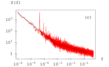
Figure 1: Trading statistics of IBM stocks. a) Histogram $P(\tau)$ of the intertrade time $\tau_{k}$ sequence; b) Histogram of trading activity $P(N)$ calculated in the time interval $\tau_{d}=10\,\mathrm{min}$; c) Power spectral density $S(f)$ of the sequence of trades, straight lines approximate power spectrum $S(f)\sim 1/f^{\beta_{1,2}}$ with $\beta_{1}=0.33$ and $\beta_{2}=0.94$.

The histograms and power spectrum of the sequences of trades for all 26 stocks are similar to IBM shown on Fig. 1. From the histogram $P(\tau_{k})$ we define a model parameter $\tau_{0}$ for every stock. One can define the exponent $\lambda^{\prime}$ from the power-law tail of the histogram $P(N)\sim N^{-\lambda^{\prime}}$. The power spectrum exhibits two scaling exponents $\beta_{1}$ and $\beta_{2}$ when approximated by power-law $S(f)\sim 1/f^{\beta_{1,2}}$. The empirical values of $\beta_{1}$, $\beta_{2}$, $\tau_{0}$ and $\lambda^{\prime}$ for $\tau_{d}=10\,\mathrm{min}$ are presented in Table 1.

Table 1: The empirical values of $\tau_{0}$, $\beta_{1}$, $\beta_{2}$ and $\lambda^{\prime}$.

Stock	$\tau_{0}$	$\beta_{1}$	$\beta_{2}$	$\lambda^{\prime}$	Stock	$\tau_{0}$	$\beta_{1}$	$\beta_{2}$	$\lambda^{\prime}$
ABT	7	0.27	0.92	5.8	JNJ	4	0.31	0.87	4.4
ADM	8	0.29	0.96	3.5	JPM	4.5	0.3	0.8	5.7
BA	8	0.32	0.84	4.5	KO	6	0.29	0.85	6.5
BMY	7	0.3	0.9	4.4	LLY	8	0.32	0.84	4.5
C	3	0.31	0.87	4.6	MMM	8	0.26	0.96	4.8
CVX	4	0.3	0.87	6.4	MO	5	0.36	0.9	3.6
DOW	7	0.32	0.88	5.7	MOT	4	0.29	0.93	3.4
FNM	9	0.36	0.95	3.4	MRK	5	0.35	0.82	3
FON	8	0.29	0.97	3.4	SLE	10	0.2	0.75	4.5
GE	2.25	0.27	0.87	4.7	PFE	2	0.31	0.96	3.6
GM	6	0.36	0.93	2.7	T	10	0.28	0.88	3.7
HD	4	0.32	0.95	5.4	WMT	4	0.31	0.84	4.7
IBM	5	0.3	0.87	4.1	XOM	3	0.34	0.9	4.4
Average						5.8	0.305	0.89	4.4

Values of $\beta_{1}$ and $\beta_{2}$ fluctuate around $0.3$ and $0.9$, respectively, as in the separate stochastic model realizations. The crossover frequency $f_{c}$ of two power-laws exhibits some fluctuations around the value $f_{c}\approx 10^{-3}\,\mathrm{Hz}$ as well. One can observe considerable fluctuations of the exponent $\lambda^{\prime}$ around the mean value $4.4$. Notice that value of exponent $\lambda^{\prime}$ for integrated trading activity $N$ is higher than for $n$. Our analysis shows that the explicit form of the $P(\tau_{k})$, Eq. (4) with $m=2$ and $\lambda=2.7$, fits empirical histogram of $\tau_{k}$ for all stocks very well and fitting parameter $\tau_{0}$ can be defined for every stock. Values of $\tau_{0}$ are presented on Table 1. From the point of view of the proposed model the parameter $\tau_{0}$ is specific for every stock and reflects the average trading intensity in the calm periods of stock exchange. We eliminate these specific differences in our model by scaling transform of Eq. (8) arriving to the nondimensional SDE (9) and its iterative form (10). These equations and parameters $\sigma^{\prime}=\sigma/\tau_{0}$, $\gamma_{\sigma}$, $\epsilon^{\prime}$ and $m=2$ define our model, which has to reproduce in details power-law statistics of the trading activity in the financial markets. From the analysis based on the research of fractal stochastic point processes [13, 14, 15, 16, 17, 18] and by fitting the numerical calculations to the empirical data we arrive at the collection of parameters $\sigma^{\prime}=0.006$, $\gamma_{\sigma}=0.64$, $\epsilon^{\prime}=0.05$. In figure 2 we present histogram of the sequence of $\tau_{k}=h_{k}$, (a), and the power spectrum of the sequence of trades as point events, (b), generated numerically by Eq. (10) with the adjusted parameters.

Figure 2: Distribution of the Poissonian-like interevent time $\tau_{k}=h_{k}$, (a), and power spectrum, (b), of the sequence of point events calculated from Eq. (10) with the adjusted parameters $\sigma^{\prime}=0.006$, $\gamma_{\sigma}=0.64$, $\epsilon^{\prime}=0.05$.

For every selected stock one can easily scale the model sequence of intertrade times $\tau_{k}=h_{k}$ by empirically defined $\tau_{0}$ to get the model sequence of trades for this stock. One can scale the model power spectrum $S(f)$ by $1/\tau_{0}^{2}$ for getting the model power spectrum $S_{\mathrm{stock}}(f)$ for the selected stock $S_{\mathrm{stock}}(f)=S(f)/\tau_{0}^{2}$.

Figure 3: Distribution $P(\tau)$ of intertrade time $\tau$ for IBM and MMM stocks; empirical histogram, tick gray line, modeled Poissonian-like distribution, solid line, distribution of driving $\tau=y_{k}$ in Eq. (10), dashed line.

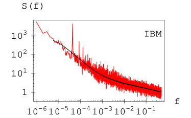
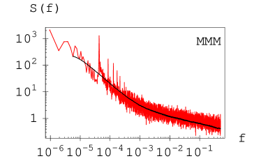
Figure 4: Modeled, smooth curves, and empirical, sharp curves, power spectra of trading activity for IBM and MMM stocks.

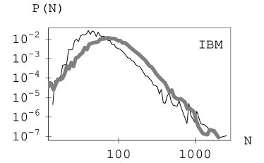
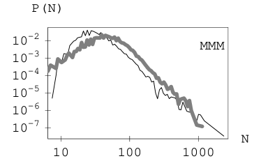
Figure 5: Modeled, thin line, and empirical, tick line, trading activities for IBM and MMM stocks in the time interval $\tau_{\mathrm{d}}=300s$.

We proposed the iterative Eq. (10) as quite accurate stochastic model of trading activity in the financial markets. Nevertheless, one has to admit that real trading activity often has considerable trend as number of shares traded and the whole activity of the markets increases. This might have considerable influence on the empirical long range distributions and power spectrum of the stocks in consideration. The trend has to be eliminated from the empirical data for the detailed comparison with the model. Only few stocks from the selected list in Table 1 have stable trading activity in the considered period. In figures 3, 4 and 5 we provide the comparison of the model with the empirical data of those stocks. As we illustrate in figure 3, the model Poissonian-like distribution can be easily adjusted to the empirical histogram of intertrade time, with $\tau_{0}=5\,\mathrm{s}$ for IBM trade sequence and with $\tau_{0}=8\,\mathrm{s}$ for MMM trading. The comparison with the empirical data is limited by the available accuracy, $1\,\mathrm{s}$, of stock trading time $t_{k}$. The probability distribution of driving $\tau=y_{k}$ Eq. (10), dashed line, illustrates different market behavior in the periods of the low and high trading activity. The Poissonian nature of the stochastic point process hides these differences by considerable smoothing of the PDF. Figure 4 illustrates that the long range memory properties of the trading activity reflected in the power spectrum are universal and arise from the scaled driving SDE (5) and (9). One can get power spectrum of the selected stock trade sequence scaling model spectrum, figure 2 (b), with $1/\tau_{0}^{2}$. The PDF of integrated trading activity $N$ is more sensitive to the market fluctuations. Nevertheless, as we demonstrate in figure 5, the model is able to reproduce the power-law tails very well.

4 Conclusions

We proposed the generalization of the point process model as the Poissonian-like sequence with slowly diffusing mean interevent time [14] and adjusted the parameters of the model to the empirical data of trading activity in the financial markets. A new form of scaled equations provides the universal description with the same parameters applicable for all stocks. The proposed new form of the continuous stochastic differential equation enabled us to reproduce the main statistical properties of the trading activity and waiting time, observable in the financial markets. In proposed model the fractured power-law distribution of spectral density with two different exponents arise. This is in agreement with the empirical power spectrum of the trading activity and volatility and implies that the market behavior may be dependent on the level of activity. One can observe at least two stages in market behavior: calm and excited. Ability to reproduce empirical PDF of intertrade time and trading activity as well as the power spectrum in every detail for various stocks provides a background for further stochastic modeling of volatility.

Acknowledgment

We acknowledge the support by the Agency for International Science and Technology Development Programs in Lithuania and EU COST Action P10 “Physics of Risk”.

References

- [1] R. Engle, Econometrica 50 (1982) 987.
- [2] T. Bollersev, Journal of Econometrics 31 (1986) 307.
- [3] R. Baillie, T. Bollersev and H.O. Mikkelsen, Journal of Econometrics 74 (1996) 3.
- [4] R. Engle and A. Patton, Quant. Finance 1 (2001) 237.
- [5] J. Perello and J. Masoliver, Phys. Rev. E 67 (2003) 037102.
- [6] J. Perello, J. Masoliver and N. Anento, Physica A 344 (2004) 134.
- [7] A. Dragulescu, V. Yakovenko, Quant. Finance 2 (2002) 443.
- [8] J.C. Hull, A. White, The Journal of Finance 42 (1987) 281.
- [9] B.B. Mandelbrot, J. Business 36 (1963) 394.
- [10] T. Lux, Appl. Fin. Econ. 6 (1996) 463.
- [11] V. Plerou, P. Gopikrishnan, X. Gabaix, L.A.N. Amaral and H.E. Stanley, Quant. Finance 1 (2001) 262.
- [12] X. Gabaix, P. Gopikrishnan, V. Plerou, H.E. Stanley, Nature 423 (2003) 267.
- [13] V. Gontis and B. Kaulakys, J. Stat. Mech. (2006) P10016.
- [14] V. Gontis and B. Kaulakys, Physica A 382 (2007) 114.
- [15] V. Gontis and B. Kaulakys, Physica A 343 (2004) 505.
- [16] V. Gontis and B. Kaulakys, Physica A 344 (2004) 128.
- [17] B. Kaulakys, V. Gontis and M. Alaburda, Phys. Rev. E 71 (2005) 051105.
- [18] B. Kaulakys, J. Ruseckas, V. Gontis and M. Alaburda, Physica A 365 (2006) 217.