The Ly$\alpha$ and Ly$\beta$ Profiles in Solar Prominences and Prominence Fine Structure

Abstract

Ly$\alpha$ and Ly$\beta$ line profiles in a solar prominence were observed with high spatial and spectral resolution with SOHO/SUMER. Within a 60 arcsec scan, we measure a very large variety of profiles: not only reversed and non-reversed profiles but also red-peaked and blue-peaked ones in both lines. Such a spatial variability is probably related to both the fine structure in prominences and the different orientations of mass motions. The usage of integrated-intensity cuts along the SUMER slit, allowed us to categorize the prominence in three regions. We computed average profiles and integrated intensities in these lines which are in the range (2.36 – 42.3) W m^-2 sr^-1 for Ly$\alpha$ and (0.027 – 0.237) W m^-2 sr^-1 for Ly$\beta$. As shown by theoretical modeling, the Ly$\alpha$/Ly$\beta$ ratio is very sensitive to geometrical and thermodynamic properties of fine structure in prominences. For some pixels, and in both lines, we found agreement between observed intensities and those predicted by one-dimensional models. But a close examination of the profiles indicated a rather systematic disagreement concerning their detailed shapes. The disagreement between observations and thread models (with ambipolar diffusion) leads us to speculate about the importance of the temperature gradient between the cool and coronal regions. This gradient could depend on the orientation of field lines as proposed by Heinzel, Anzer, and Gunár (2005).

1 Introduction.

Hydrogen lines are the most prominent lines observed in solar prominences. The resonance lines of the Lyman series have been observed since the Skylab ATM experiment. The full profiles of the Ly$\alpha$ and Ly$\beta$ lines were obtained with the UV polychromator on OSO 8 for the first time in a quiescent prominence by Vial, 1982a. Both were reversed and the Ly$\alpha$ intensity was about equal to the incident chromospheric intensity multiplied by the dilution factor. The opacities are very high and radiation transfer is dominated by the scattering of chromospheric Ly$\alpha$ and Ly$\beta$ photons. The Ly$\alpha$ line has been extensively used as a diagnostic tool in the quiet or active chromosphere and especially in solar prominences (Vial, 1982b). Schmieder et al. (1999) and Heinzel et al. (2001) presented a nearly simultaneous observation of the whole Lyman series including the Ly$\alpha$ and Ly$\beta$ lines. But the Ly$\alpha$ line profile was affected by the detector attenuator.
The Ly$\alpha$/Ly$\beta$ ratio is very sensitive to the physical and geometrical properties of fine structures and consequently it provides a diagnostic tool for deriving the fine structure of solar prominences (Vial et al., 1989; Rovira et al., 1994; Fontenla et al., 1996; Heinzel et al., 2001). Non-LTE radiative transfer modeling of prominences using plane-parallel infinite slabs by Gouttebroze, Heinzel, and Vial (1993, hereafter GHV) yielded large values for this ratio (90 to 400) contrary to the OSO 8 observed value (65). Fontenla and Rovira (1983, 1985) and Vial et al. (1989) constructed thread models and solved simultaneously the radiative transfer, statistical equilibrium, and ionization equations assuming a three-level atom plus continuum. Their results showed that the Ly$\alpha$ intensities are in agreement with observations, but the Ly$\beta$ line intensities are too small compared with those observed by OSO 8 (Vial, 1982a). For strongly reversed profiles observed by SOHO/SUMER, Heinzel et al. (2001) also used multithread models and arrived at a remarkable agreement with the observed line profiles and integrated intensities for the first members of the Lyman series. Fontenla et al. (1996) considered a collection of threads in energy balance with the surrounding corona. They also took into account ambipolar diffusion. They found that ambipolar diffusion increases the emission in Ly$\beta$ in comparison with other lines in the Lyman series leading to a small Ly$\alpha$/Ly$\beta$ ratio compared to observations.
Engvold (1976), Engvold and Malville (1977) and Engvold, Malville, and Livingston (1978) observed the fine structure of non-spot prominences with H$\alpha$ filtergrams. The size of the smallest prominence structures increases with height above the chromosphere. Some prominences contain structures close to 350 km, which is the spatial resolution in these filtergrams. Some bright threads are visible for one hour and longer. Their average line-of-sight velocity is about 30 km s^-1 and their angular sizes are 1 Mm. Engvold (1978) observed five hedgerow prominences with high spatial resolution and studied some lines properties in them. He reported that the faint structures appeared slightly hotter than the bright structures. Under good seeing conditions, the quiescent prominences resolve into a fine structure that consists of narrow threads and knots. These structures are thought to arise from small-scale magnetic fields embedded within the prominence, although a direct demonstration of this connection has not yet been possible, for lack of observations with sufficient spatial resolution (Zirker and Koutchmy, 1990). The presence of fine structure must play an essential role in the transfer of radiation, and possibly, heat conduction from the corona (Zirker and Koutchmy, 1991). The cool threads may have their own transition regions to the corona (see, e.g., Heinzel (2007) or they may be embedded in a common transition region or they may be isothermal threads each having different temperatures as suggested by Poland and Tandberg-Hansen (1983). Pojoga, Nikoghossian, and Mouradian (1998) studied the possible geometries of prominence fine structures. Rovira et al. (1994) and Fontenla et al. (1996) constructed thread modeling with ambipolar diffusion and they assumed that each thread can be independently computed from its own characteristics. The effect of radiative interaction of a number of threads has been addressed by Heinzel (1989). Ajabshirizadeh and Ebadi (2005) and Ajabshirizadeh, Nikoghossian, and Ebadi (2007) used the method of addition of layers and calculated line profiles and intensity fluctuations which mainly represent the fine structure properties. Anzer and Heinzel (1999) presented slab models for quiescent prominences in which both the condition of magneto-hydrostatic equilibrium as well as Non-LTE are fulfilled. They used the Kippenhahn-Schl$\ddot{u}$ter model (Kippenhahn and Schl$\ddot{u}$ter, 1957) and deduced relations between the components of the magnetic field, gas pressure, and prominence width. Heinzel and Anzer (2001) constructed theoretical models for vertical prominence threads which are in magneto-hydrostatic equilibrium. Their models were fully two-dimensional and took the form of vertically infinite threads hanging in a horizontal magnetic field. They have shown that the Lyman profiles are more reversed when seen along the lines, a behavior recently confirmed observationally by Schmieder et al. (2007). They showed the effects of line-profile averaging over the fine structure threads which are below the instrumental resolution. Heinzel and Anzer (2003) and Heinzel, Anzer, and Gunár (2005) deduced that magnetically-confined structures in solar prominences exhibit a large complexity in their shapes and physical conditions. Since different Lyman lines and their line center, peak and wings are formed at different depths within the thread, the Lyman series may serve as a good diagnostic tool for thermodynamic conditions varying from central cool parts to a prominence-corona transition region (PCTR). They confirmed that the Lyman line profiles are more reversed when seen across the field lines, compared to those seen along the lines.
In Section 2 we present the SUMER observations of Ly$\alpha$ and Ly$\beta$ and the full information about the data that we used. Section 3 describes the data processing methods and software that we used through this work. Our results are presented in Section 4. It contains the cuts along the slit, Ly$\alpha$ and Ly$\beta$ profiles and their ratios in different regions which correspond to the studied prominence. Comparison of our results with previous works is done in Section 5 and conclusions are presented in Section 6.

2 Observations

SUMER is a high-resolution normal incidence spectrograph operating in the range (780 – 1610) Å (first order) and (390 – 805) Å (second order). The spatial resolution along the slit is 1${}^{{}^{\prime\prime}}$. The spectral resolution depends slightly on the wavelength. It can vary from about 45 mÅ per pixel at 800 Å to about 41 mÅ per pixel at 1600 Å (Wilhelm et al., 1995). A prominence situated at the limb in the north east quadrant was observed with SUMER (detector A) on 25 May 2005. Figure 1 shows the Ca II K₃ (Meudon Observatory) and 304 Å (SOHO/EIT) images of the prominence at the time of our data. It shows that the SUMER slit was well located for the prominence. The pointing coordinates were X = 972${}^{{}^{\prime\prime}}$, Y = 168${}^{{}^{\prime\prime}}$. The slit which is used was 0.3${}^{{}^{\prime\prime}}$$\times$120${}^{{}^{\prime\prime}}$. The observation was performed from 16:23 UT to 16:26 UT for Ly$\alpha$ and from 16:20 UT to 16:22 UT for Ly$\beta$. It is clear that the Ly$\alpha$ and Ly$\beta$ observations are simultaneous within a couple of minutes. The exposure time for both of them was 115 seconds. The spectral resolution is 43.67 mÅ and 44.37 mÅ for Ly$\alpha$ and Ly$\beta$ respectively. The Ly$\alpha$ observations were performed in a special mode where the gain of the detector was lowered in order to keep linearity for such an intense signal.

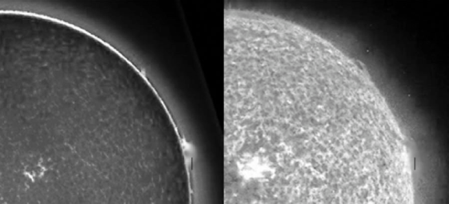
Figure 1: Images of the studied prominence which were observed by Meudon (Ca II K₃ observatory (left) and 304 Å SOHO/EIT (right) on 25 May 2005. The slit is in the North – South direction.

3 Data Processing

The raw data have been initially processed applying the standard procedures for geometric distortion, flat-fielding, and dead-time correction which can be found in the Solar Software (SSW) database. Once these corrections were applied, we performed the radiometric calibration via the radiometry program in the SSW environment. The specific intensity unit is W m^-2 sr^-1 Å^-1 through this analysis. Because of the above-mentioned special observing mode of the Ly$\alpha$ line, low signals may well be underestimated by about ten per cent according to P. Lemaire (private communication). This means that only the Ly$\alpha$ wings may be affected.

4 Results

We calculated the integrated intensities for both Ly$\alpha$ and Ly$\beta$ along the slit (Figure 2).

Figure 2: The integrated intensity along the slit for Ly$\alpha$ (left) and for Ly$\beta$ (right). There exist three regions with different intensities both in Ly$\alpha$ and Ly$\beta$ lines.

Only pixels 60 to 120 are useable. The intensities were compared with previous works and they are in the prominence range. We present Ly$\alpha$ profiles in Figures 3 and 4 and Ly$\beta$ ones in Figures 5 and 6. The numbers above each profile correspond to the position along the slit. Ly$\alpha$ line profiles from pixels 60 to 84 are non-reversed but from pixels 85 to 119 they are reversed and the reversals are more apparent in the last pixels. The intensities are increasing at the end of the slit in both lines. The reversed profiles in the case of Ly$\beta$ are located from pixels 100 to 119. Some profiles are red-shifted and some of them are blue-shifted in both lines. In some cases a significant blue peak in Ly$\alpha$ coincides with a significant red peak in Ly$\beta$ (e.g. pixels 104 and 105), but the opposite is true for pixels 110 and 115.
As Figure 2 shows, there are three regions with different intensities, so we decided to study the prominence in three categories which are called P-1, P-2, and P-3.
We plotted Ly$\alpha$ and Ly$\beta$ average profiles separately for each region in Figures 7 and 8. Ly$\alpha$ line is reversed in regions P-2 and P-3, but Ly$\beta$ is reversed only in P-3. From P-1 to P-3 the average intensities and line widths increase in both lines.

Figure 3: Ly$\alpha$ profiles from pixels 62 to 89 along the slit.

Figure 4: Ly$\alpha$ profiles from pixels 90 to 119 along the slit.

Figure 5: Ly$\beta$ profiles from pixels 62 to 89 along the slit.

Figure 6: Ly$\beta$ profiles from pixels 90 to 119 along the slit.

Figure 7: Ly$\alpha$ average profiles for the three regions.

Figure 8: Ly$\beta$ average profiles for the three regions.

The Ly$\alpha$/Ly$\beta$ ratio for the three regions is presented in Figure 9. The ratio in P-1 is smaller than in the other regions. This ratio has fluctuations (12, 5, and 3 percent for P-1, P-2, and P-3 regions respectively) which are related to prominence fine structure. A summary of our Ly$\alpha$ and Ly$\beta$ intensities and their ratio is presented in Table I where they are compared to OSO 8 observations. Only the P-2 and P-3 Ly$\alpha$ and Ly$\beta$ intensities are comparable (but not equal) to OSO 8 results. However, because of the high OSO 8 Ly$\beta$ intensity, the OSO 8 Ly$\alpha$/Ly$\beta$ ratio is lower than ours by a factor three. We are confident in our measurements made with high statistics, specially in P-3. In terms of photometric calibration, OSO 8 and SUMER refer to the same disk absolute intensities (for Ly$\alpha$ and Ly$\beta$ respectively). We can only speculate that the SUMER and OSO 8 observations were of very different structures.

Table 1: The observed integrated intensities of Ly$\alpha$ and Ly$\beta$ and their ratio.

Prominence region	Ly$\alpha$ (W m-2 sr-1)	Ly$\beta$ (W m-2 sr-1)	Ly$\alpha$/Ly$\beta$
P-1	x2.36	0.027	x96
P-2	15.87	0.089	183
P-3	42.30	0.237	181
OSO 8 observations (Vial, 1982a)	28 – 36	0.44 – 0.55	x65

Figure 9: Ly$\alpha$/Ly$\beta$ for the three regions (P-1, P-2 and P-3 from left to right).

5 Comparison with the Fine Structure Modeling

We observed different profiles with different intensities both in Ly$\alpha$ and Ly$\beta$ which provide evidence of fine structuring in solar prominences. We now compare these results (in terms of integrated intensities), with non-LTE modeling. Non-LTE radiative transfer modeling of prominences has been performed using plane-parallel finite slabs by Gouttebroze, Heinzel, and Vial (1993). We selected some pixels along the slit and managed to find GHV models which match Ly$\alpha$ and Ly$\beta$ integrated intensities. They are described in Table II where the first column provides the pixel number and the last three columns describe the relevant model. The range of fitting models is rather large, from low temperature and low pressure models (8000 K and 0.01 dyn cm^-2) to higher temperature and pressure ones (10000 K, 0.2 dyn cm^-2), most of them being relatively thick (5000 km). We noticed that bright regions are well fitted by models with low temperature, high pressure and important geometrical thickness. But these model agreements become rather illusory when one looks at the actual shapes of the observed and computed profiles. The comparison is performed in Table II where columns 2 and 3 each represent the nature of the observed and modeled Ly$\alpha$ and Ly$\beta$ profiles, respectively. U means unreversed, R means reversed and F flat-topped. One can see that the only agreement for both lines is attained at pixels 107 and 110, where all profiles are actually reversed. Let us also note that all other profiles of Table II are NOT reversed, contrary to observations of Vial, 1982a. Such a discrepancy could be interpreted in terms of the modeling of prominence fine structures by Heinzel, Anzer, and Gunár (2005): These authors found that the Lyman line profiles are much more reversed when seen across the field lines, compared to those seen along the lines. The agreement between observed and modeled maximum intensities (columns 4 and 5) is rather good. The agreement between observed and modeled full widths at half maximum (FWHM) (columns 6 and 7) is generally excellent at the exception of a few ratios of 0.5. But maximum intensities and FWHM represent crude parameters of lines profiles whose general observation/modeling agreement complies with the integrated intensities agreement. Returning now to the issue of integrated intensities, we also compared with systems of thread models.
Fontenla and Rovira (1983, 1985) and Vial et al. (1989) developed non-LTE models of individual prominence threads including a large number of narrow threads. They found that the computed Ly$\alpha$ profiles are close to the observed ones, but the Ly$\beta$ line intensities are too small and consequently, the Ly$\alpha$/Ly$\beta$ ratio is high compared with that observed by OSO 8 (Vial, 1982a). More recently, Fontenla et al. (1996) found that ambipolar diffusion increases the emission in Ly$\beta$ in comparison with other lines in Lyman series. However, the ambipolar diffusion models give excessive Ly$\beta$ emission, viz., too small a Ly$\alpha$/Ly$\beta$ ratio compared with observations. Table III presents a comparison of theoretical modeling results including integrated intensities of Ly$\alpha$ and Ly$\beta$ and their ratio with our results. Although we find some agreement with the 1D models of Gouttebroze, Heinzel, and Vial (1993) and thread modeling without ambipolar diffusion (Fontenla and Rovira, 1983, 1985; Vial et al., 1989), we have no agreement with thread modeling with ambipolar diffusion (Fontenla et al., 1996).
The spatial variations of the integrated Ly$\alpha$ and Ly$\beta$ intensities and their ratio could only be matched by a variety of 1D models, although the detailed shapes of the profiles did not match (see Table II). The variety of fitting models and their inadequacy for profile shapes are a strong indication of the existence of a fine structure where the cool core must be complemented with some kind of PCTR. Moreover, the recent Swedish Solar Telescope observations of Lin et al. (2005) present unescapable evidence of fine structures as one can see by looking at the images. Actually, the possibility of having an agreement with thread models without ambipolar diffusion indicates that the temperature gradient at the boundary of prominence threads may not be as strong as in the chromosphere-corona transition region (and consequently the ambipolar diffusion less efficient). Such a conclusion was already reached by Chiuderi and Chiuderi-Drago (1991). Heinzel, Anzer, and Gunár (2005) also reached a similar conclusion in terms of profile variations along (across) the magnetic field lines, where conduction is parallel (perpendicular), respectively. Unfortunately, because of insufficient geometrical information on the magnetic structure of the prominence we observed and also because of the projection effects when a prominence is seen at the limb, we cannot assign our spatial observations to a particular orientation of our line of sight with respect to the field lines.

Table 2: Gouttebroze, Heinzel, and Vial (1993) 1Dimensional model results which are in agreement with our observations. Column 1 presents the pixels along the SUMER slit and S1 and S2 are the shapes of observed vs. modeled profiles for Ly$\alpha$ and Ly$\beta$ respectively. U means unreversed, F flat-topped and R reversed. I₁ and I₂ are the ratio of observed maximum intensities to the computed ones relevant to this model for Ly$\alpha$ and Ly$\beta$ respectively. F1 and F2 are the ratio of the observed FWHM to computed one for Ly$\alpha$ and Ly$\beta$ lines respectively. R${}_{\mbox{OC}}$ is the ratio of the observed Ly$\alpha$/Ly$\beta$ integrated intensities to the computed ones. Three last columns present the model parameters (temperature (K), pressure (dyn cm^-2) and geometrical thickness (km)).

Pixel	S1	S2	I1	I2	F1	F2	R${}_{\mbox{OC}}$	T	P	$\Delta z$
85	U/R	F/U	1.0	0.8	1.1	1.3	0.8	x8000	0.01	5000
86	U/R	U/U	1.1	0.9	0.8	1.4	1.0	x8000	0.01	1000
90	U/R	U/R	1.0	1.0	0.5	1.1	0.5	x8000	0.20	1000
93	U/R	U/U	1.0	1.1	0.5	1.0	0.6	x8000	0.01	5000
99	F/R	U/F	1.1	0.9	1.1	1.3	0.9	x8000	0.20	x200
100	F/R	U/R	1.0	0.9	1.5	1.3	1.4	15000	0.01	5000
102	F/R	U/F	1.0	0.8	0.8	1.3	0.6	x8000	0.20	x200
107	R/R	R/R	1.0	1.0	1.2	1.0	0.8	10000	0.05	5000
110	R/R	R/R	0.9	0.9	1.5	1.5	0.8	10000	0.20	x200
111	F/R	F/R	1.1	0.8	0.6	1.1	0.7	x8000	0.20	5000

Table 3: Integrated intensities of Ly$\alpha$ and Ly$\beta$ and their ratio (1: Our results, 2: Gouttebroze, Heinzel, and Vial (1993), 3: Fontenla and Rovira (1983, 1985) and Vial et al. (1989) 4: Fontenla et al. (1996)).

Reference	Ly$\alpha$ (W m-2 sr-1)	Ly$\beta$ (W m-2 sr-1)	Ly$\alpha$/Ly$\beta$
SUMER observations (1)	xx2.36 – 42.3	0.027 – 0.237	96 – 180
One-dimensional Modeling (2)	x7.50 – 45	0.037 – 0.29	90 – 400
Thread modeling without A.D. (3)	13.60 – 55	0.1 – 1.3	42 – 111
Thread modeling with A.D. (4)	x10.80 – 38.6	0.59 – 7.36	2.3 – 18.5

6 Conclusions

We have presented nearly simultaneous Ly$\alpha$ and Ly$\beta$ profiles obtained in a prominence with the SUMER spectrograph on SOHO. Significant variability of these profiles on scales as small as 1^′′ is present. Reversed and unreversed profiles were obtained in both lines with behaviors which differ from one line to the other (e.g. significant blue peak in Ly$\alpha$ coinciding with a significant red peak in Ly$\beta$). Although the number of observed profiles is limited to about 60, making a proper statistical analysis impossible, we believe that such spectral signatures result from fine structuring of prominences. In bright regions of the prominence, the Ly$\alpha$ intensity is larger than the OSO-8 value, and the Ly$\beta$ intensity is lower. We have some agreements with one-dimensional models and thread models without ambipolar diffusion, but thread modeling with ambipolar diffusion gives high Ly$\beta$ intensity and as a result too small a ratio. Such a result indicates that the temperature gradient at the boundary of threads may not be as strong as in the 1D PCTR models or that the magnetic field direction has a profound influence on the profiles (as shown by Heinzel, Anzer, and Gunár (2005)). Actually, a detailed comparison between some observed and 1D-modeled profiles(see Table II) supports this idea. Note that the same data as used in this paper were recently analyzed in terms of 2D fine structure models in magnetohydrostatic equilibrium and fitting the line profiles of the Lyman series has pointed to multithreads seen across the magnetic field lines giving rise to reversed profiles (Gunár et al. 2007). A combination of spectral and imaging information in the Lyman series (in particular the Ly$\alpha$ and Ly$\beta$ lines) would be a still more efficient tool for deriving the actual fine structure of prominences.

Acknowledgments: The authors thank P. Lemaire, F. Baudin, P. Boumier, K. Wilhelm, and K. Bocchialini for useful comments on the data processing, and J. Leibacher for his help in improving the manuscript. They warmly thank the anonymous referee for help in improving the document. The observations took place in the frame of the 15th MEDOC Campaign. The authors thank all MEDOC Campaign participants, especially K. Wilhelm, B. Schmieder, and P. Schwartz for their contribution to the Campaign. SUMER is financially supported by DLR, CNES, NASA, and the ESA PRODEX program (Swiss contribution). SOHO is a mission of international cooperation between ESA and NASA.

References

- [1] Ajabshirizadeh, A. and Ebadi, H.: 2005, J. Quant. Spectrosc. Radiat. Transfer 95, 127.
- [2] Ajabshirizadeh, A., Nikoghossian, A.G., and Ebadi, H.: 2007, J. Quant. Spectrosc. Radiat. Transfer 103, 351.
- [3] Anzer, U. and Heinzel, P.: 1999, Astron. Astrophys. 349, 794.
- [4] Chiuderi, C. and Chiuderi-Drago F.: 1991, Solar Phys.132 , 81.
- [5] Engvold, O.: 1976, Solar Phys. 49, 283.
- [6] Engvold, O.: 1978, Solar Phys. 56, 87.
- [7] Engvold, O. and Malville, J.M.: 1977, Solar Phys. 52, 369.
- [8] Engvold, O., Malville, J.M., and Livingston, W.: 1978, Solar Phys. 60, 57.
- [9] Fontenla, J. M. and Rovira, M.: 1983, Solar Phys. 85, 141.
- [10] Fontenla, J. M. and Rovira, M.: 1985, Solar Phys. 96, 53.
- [11] Fontenla, J.M., Rovira, M., Vial, J.-C., and Gouttebroze, P.: 1996, Astrophy. J. 466, 496.
- [12] Gouttebroze, P., Heinzel, P., and Vial, J. C.: 1993, Astron. Astrophys. 99, 513 (GHV).
- [13] Gunár, S., Heinzel, P., Schmieder, B., and Anzer, U.: 2007, In: Heinzel, P., Dorotovic, I., Rutten, R.J. (eds.), The Physics of Chromospheric Plasmas, Astron. Soc. Pacific Conf. Ser., San Francisco 368, 317.
- [14] Heinzel, P.: 1989, Hvar Obs. Bull. 13, 317.
- [15] Heinzel, P.: 2007, In: Heinzel, P., Dorotovic, I., Rutten, R.J. (eds.), The Physics of Chromospheric Plasmas, Astron. Soc. Pacific Conf. Ser., San Francisco 368, 271.
- [16] Heinzel, P. and Anzer, U.: 2001, Astron. Astrophys. 375, 1082.
- [17] Heinzel, P. and Anzer, U.: 2003, In: Hubeny, D., Mihalas, D., Werner, K. (eds), Stellar Atmosphere Modeling, Astron. Soc. Pacific Conf. Ser., San Francisco 288, 441.
- [18] Heinzel, P., Anzer, U., and Gunár, S.: 2005, Astron. Astrophys. 442, 331.
- [19] Heinzel, P., Schmieder, B., Vial, J.-C., and Kotrc, P.: 2001, Astron. Astrophys. 370, 281.
- [20] Kippenhahn, R. and Schlter, A.: 1957, Z. Astrophys. 43, 36.
- [21] Lin, Y., Engvold, O., Rouppe, L., Wiik, J.-E., and Berger, T.-E.: 2005, Solar Phys. 226, 239.
- [22] Pojoga, S., Nikoghossian, A. G., and Mouradian, Z.: 1998, Astron. Astrophys. 332, 325.
- [23] Poland, A.I. and Tandberg-Hansen, E.: 1983, Solar Phys. 84, 63.
- [24] Rovira, M. G., Fontenla, J. M., Vial, J.-C., and Gouttebroze, P.: 1994, In: Rusin, V., Heinzel, P., and Vial J.-C. (eds.), Solar Coronal Structures, IAU Colloq., VEDA Publish. Comp., Bratislava 144, 315.
- [25] Schmieder, B., Heinzel, P., Vial, J.-C., and Rudway, P.: 1999, Solar Phys. 189, 109.
- [26] Schmieder, B., Gunár, S., Heinzel, P., and Anzer, U.: 2007, Solar Phys. 241, 53.
- [27] Vial, J.-C.: 1982a, Astrophy. J. 253, 330.
- [28] Vial, J.-C.: 1982b, Astrophy. J. 254, 780.
- [29] Vial, J.-C., Rovira, M.G., Fontenla, J.M., and Gouttebroze, P.: 1989, Hvar Obs. Bull., 13(1), 331.
- [30] Wilhelm, K., Curdt, W., Marsch, E., Schhle, U., Lemaire, P., Gabriel, A., et al.: 1995, Solar Phys. 162, 189.
- [31] Zirker, J.B. and Koutchmy, S.: 1990, Solar Phys.127, 109.
- [32] Zirker, J.B. and Koutchmy, S.: 1991, Solar Phys.131, 107.