High-resolution polarimetry of Parsamian 21: revealing the structure of an edge-on FU Ori disc

Abstract

We present the first high spatial resolution near-infrared direct and polarimetric observations of Parsamian 21, obtained with the VLT/NACO instrument. We complemented these measurements with archival infrared observations, such as HST/WFPC2 imaging, HST/NICMOS polarimetry, Spitzer IRAC and MIPS photometry, Spitzer IRS spectroscopy as well as ISO photometry. Our main conclusions are the following: (1) we argue that Parsamian 21 is probably an FU Orionis-type object; (2) Parsamian 21 is not associated with any rich cluster of young stars; (3) our measurements reveal a circumstellar envelope, a polar cavity and an edge-on disc; the disc seems to be geometrically flat and extends from approximately 48 to 360 AU from the star; (4) the SED can be reproduced with a simple model of a circumstellar disc and an envelope; (5) within the framework of an evolutionary sequence of FUors proposed by Green et al. (2006) and Quanz et al. (2007), Parsamian 21 can be classified as an intermediate-aged object.

1 Introduction

The most important process of low-mass star formation is the accretion of circumstellar material onto the young star. According to current models, the mass accumulation is time-dependent with alternating episodes of high and low accretion rates (Vorobyov & Basu, 2006; Boley et al., 2006). The high phase may correspond to FU Orionis objects (FUors), a unique class of low-mass pre-main sequence stars that have undergone a major outburst in optical light of $4\,$mag or more (Herbig, 1977). Currently about 20 objects have been classified as FU Ori-type (for a list see Ábrahám et al., 2004). Records of the outbursts are not available for all of these objects: some were classified as FUors since they share many spectral properties with the FUor prototypes. According to the most widely accepted model (Kenyon & Hartmann, 1991), the observed spectral energy distribution (SED) is reproduced by a combination of an accretion disc and an envelope. The energy of the outburst originates from the dramatic increase of the accretion rate. On the other hand, Herbig et al. (2003) favour a model in which the outburst occurs in an unstable young star rotating near breakup velocity.

Parsamian 21 is a system consisting of a central object, HBC 687 ($\alpha_{2000}$ = 19^h 29^m 0$\aas@@fstack{s}$87, $\delta_{2000}$ = 9° 38′ 42$\aas@@fstack{\prime\prime}$69), and an extended nebula first listed in the catalogue of Parsamian (1965). Though no optical outburst was ever observed, Parsamian 21 was classified as a FUor on the basis of its optical spectroscopic and far-infrared properties (Staude & Neckel, 1992). According to Henning et al. (1998) Parsamian 21 is situated in a molecular cloud named “Cloud A”, very close to the Galactic plane. Indeed, the distance of 400 pc and the radial velocity of $v_{lsr}=+27\pm 15$ km s^-1 (Staude & Neckel, 1992) agree very well with the respective values for Cloud A ($v_{lsr}=+27\pm 4$ km s^-1, $d=500\pm 100$ pc, Dame & Thaddeus, 1985). Recently Quanz et al. (2007) questioned the FUor nature of Parsamian 21 referring to mid-infrared spectral properties, which better resemble those of post-AGB stars (this issue will be discussed in Sect. 4).

The elongated nebulosity around the central source extends ${\approx}\,1\,$arcmin to the north, while it is less developed to the south. It is visible in the optical and the near-infrared, though the source becomes unresolved at $10.8$ and $18.2\,\mu$m (Polomski et al., 2005). Polarimetric observations by Draper et al. (1985) revealed a centrosymmetric polarization pattern and an elongated band of low polarization perpendicular to the axis of the bright nebula. Bastien & Ménard (1990) interpreted the polarization map of Parsamian 21 in terms of multiple scattering in flattened, optically thick structures and derived an inclination angle of 80-85° and a size of 30 $\times$ 8 arcsec for this disc-like structure. The existence of a disc is also supported by the discovery of a short bipolar outflow oriented along the polar axis of the nebula (Staude & Neckel, 1992). Emission at submm wavelengths was detected by Henning et al. (1998) and Polomski et al. (2005). The surroundings of Parsamian 21 have been searched for companions several times, but close-by stars seen in J, H and K-band images proved to be field stars (Li et al., 1994), and no close-by sources have been found at longer wavelengths so far (Polomski et al., 2005).

Recently several studies were published on the circumstellar environment of FUors using high-resolution infrared and interferometric techniques (e.g. Green et al. 2006; Malbet et al. 1998, 2005; Millan-Gabet et al. 2006a; Quanz et al. 2007). Such observations could prove or disprove the basic assumptions of FUor models. In this paper we present the highest resolution imaging and polarimetric data yet on Parsamian 21 from the VLT/NACO instrument, allowing the inspection of the circumstellar material and disc at spatial scales of ${\approx}\,0.07$ arcsec. The edge-on geometry of Parsamian 21 represent an ideal configuration to separate the components of the circumstellar environment (disc, envelope) and understand their role in the FUor phenomenon.

2 Observations and data reduction

The log of observations presented in this paper is summarized in Table 1. In the following subsections we describe these measurements in detail.

2.1 VLT/NACO observations

We have acquired ground-based near-infrared imaging and polarimetric observations in visitor mode using the NACO instrument mounted on the UT4 of ESO’s Very Large Telescope VLT at Cerro Paranal, Chile on 2004 June 18. NACO consists of the NAOS adaptive optics system and the CONICA near-infrared camera (Lenzen et al., 1998; Hartung et al., 2000; Rousset et al., 2003). The weather conditions were excellent, the typical optical seeing was $\approx 0.72$ arcsec with two short peaks of $1.3$ arcsec during the night. For imaging we used the visual dichroic and a camera with 13 mas/pixel scale to obtain H ($\lambda_{\mathrm{c}}=1.66\,\mu$m) and K_S ($\lambda_{\mathrm{c}}=2.18\,\mu$m) images and a camera with 27 mas/pixel scale to obtain L^′ ($\lambda_{\mathrm{c}}=3.8\,\mu$m) images. In each filter a 4-point dithering was applied with small-amplitude random jitter at each location. The adaptive optics configuration was fine-tuned for each filter to ensure the best possible correction. The H-band polarimetric observations were obtained using the 27 mas/pixel scale camera.

Table 1: Log of the observations of Parsamian 21. Top part: data from this paper; Bottom part: archival data.

Instrument	Filter (central $\lambda$)	Mode	Date	Exp. Time	Field of View	Pixel scale	FWHM
			YY/MM/DD		[arcsec $\times$ arcsec]	[arcsec]	[arcsec]
VLT/NACO	H ($1.66\,\mu$m)	Imaging	04/06/18	8$\times$30 s	13.6$\times$13.6	0.013	0.07
VLT/NACO	KS ($2.18\,\mu$m)	Imaging	04/06/18	8$\times$20 s	13.6$\times$13.6	0.013	0.07
VLT/NACO	L′ ($3.80\,\mu$m)	Imaging	04/06/18	48$\times$0.2 s	27.8$\times$27.8	0.027	0.11
VLT/NACO	H (1.66 $\mu$m)	Polarimetry	04/06/18	72$\times$10 s, 24$\times$80 s	27.8$\times$3.1	0.027	0.12
GFP	6563 and 6590Å	Imaging	07/05/15	900 s	130 circular	0.38	1.1
HST/NICMOS	$2\,\mu$m	Polarimetry	97/11/12	18$\times$31 s	19.5$\times$19.3	0.076	0.16
HST/WFPC2	F814W ($0.80\,\mu$m)	Imaging	01/07/30	2$\times$500 s	79.5$\times$79.5	0.1	0.17
Spitzer/IRAC	$3.6$, $4.5$, $5.8$ and $8.0\,\mu$m	Imaging	04/04/21	848 s	318$\times$318	1.2	1.9–2.7
Spitzer/MIPS	$24$ and $70\,\mu$m	Imaging	04/04/13	73 s, 462 s	444$\times$480, 174$\times$192	2.5, 4.0	6, 18
Spitzer/IRS	$5-40\,\mu$m	Spectroscopy	04/04/18	1121 s
ISO/ISOPHOT	$65$ and $100\,\mu$m	Imaging	96/09/28	3542 s	360$\times$420	15	44, 47

VLT/NACO imaging.

The data reduction was carried out using self-developed IDL routines. For the H and K_S band filters lampflats were taken, while for the L^′ filter, skyflats were acquired. For each filter, these images were combined to a final flatfield, and bad pixel maps were produced. Then the raw images were flatfield corrected, and bad pixels were removed. Sky frames were calculated by taking the median of all images taken with the same filter, then images were sky subtracted. Individual frames were shifted to the same position and their median was taken to obtain the final mosaic. Shifts were calculated by computing the cross-correlation of the images, which gives a more precise result in case of extended sources, than a simple Gaussian-fitting to the peak. Dithering resulted in a final mosaic of $21.4\,{\times}\,21.4$ arcsec in case of H and K_S band, and $43.8\,{\times}\,43.8$ arcsec in L^′ band. The photometric standard was S889-E for the H and K_S filters (H$\,{=}\,11.662\,{\pm}\,0.004$ mag, K${}_{S}\,{=}\,11.585\,{\pm}\,0.005$ mag, Persson et al. 1998), and HD 205772 for the L^′ filter (L${}^{\prime}\,{=}\,7.636\,{\pm}\,0.027$ mag, Bouchet et al. 1991).

VLT/NACO polarimetry.

Polarimetric observations were obtained using the differential polarimetric imaging technique (DPI, see e.g. Draper et al., 1985; Kuhn et al., 2001; Apai et al., 2004). The basic idea of this method is to take the difference of two orthogonally polarized, simultaneously acquired images of the same object in order to remove all non-polarized light. As the non-polarized light mainly comes from the central star, after subtraction only the polarized light, such as the scattered light from the circumstellar material remains. This standard way of dual-beam imaging polarimetry combined with adaptive optics at the VLT is a powerful way of doing high-contrast mapping. We obtained polarimetric images with NACO through the H filter, using a Wollaston prism with a 2 arcsec Wollaston mask to exclude overlapping beams of orthogonal polarization. Parsamian 21 was observed at four different rotator angles of 0^∘, 45^∘, 90^∘ and 135^∘, providing a redundant sampling of the polarization vectors. At each angle a 3-point dithering was applied. The polarimetric calibrator was R CrA DC No. 71 (Whittet et al., 1992). The polarimetric data reduction was done in IDL using previously developed software tools which we presented in detail in Apai et al. (2004). According to the NACO User’s Manual, instrumental polarization is generally about 2%. Based on our polarimetric calibration measurements, we found a typical instrumental polarization value of 3% (position angle: 91^∘ east of north). Considering the expected high polarization for the Parsamian 21 nebula, we can conclude that instrumental polarization can be neglected in the present case, except in limited areas of low polarization.

2.2 GFP H_α imagery

Parsamian 21 was observed with the Goddard Fabry-Perot (GFP) interferometer at the Apache Point Observatory 3.5m telescope on 2007 May 15. The observations were made in direct imaging mode. The on-band image has a central wavelength of 6563 Å (H_α) and a width of 120 km s^-1. The off-band image has a central wavelength of 6590 Å and a width of 120 km s^-1. The pixel scale is 0.38 arcsec per pixel. The observations were made through patchy cirrus and are not photometric, with seeing near 1 arcsec. The instrument and data reduction are described in Wassell et al. (2006) and references therein. For the H_α on-band image, conspicuous night sky rings contaminate the region near Par 21. In order to remove these rings, we created a data cube consisting of subimages centred on the GFP optical axis, rotated by different angles. After excluding the area around Parsamian 21, we azimuthally medianed the subimages, and subtracted the resulting image from the original measurement. For the off-band image, the night sky rings had displaced beyond the location of the Par 21 nebulosity, thus no ring subtraction was necessary. The on- and off-band images were shifted and scaled to match each other by measuring the positions and fluxes of seven stars in the vicinity of Parsamian 21. The continuum-subtracted H_α image can be seen in Fig. 3.

2.3 HST archival data

HST/NICMOS

polarimetric observations were obtained on 1997 November 12 using the NIC2 camera in MULTIACCUM mode, and the POL0L, POL120L and POL240L polarizing filters. These filters have a bandpass between $1.9$ and $2.1\,\mu$m. Raw data files were calibrated at the STScI with the calnica v.4.1.1 pipeline. Since these data have not been published yet, we downloaded the pipeline-processed files and we did further processing using the IDL-based Polarizer Data Analysis Software, which is available through the STScI website and is described by Mazzuca & Hines (1999). This software package combines the images obtained through the three polarizers using an algorithm described in Hines et al. (2000). We used coefficients appropriate for the pre-NCS measurements from Hines & Schneider (2006). A 6-point dither pattern was applied, covering in all about $24\,{\times}\,34$ arcsec. The central star and the inner parts of the Parsamian 21 nebula can only be seen in two of the six images, which we shifted and co-added.

HST/WFPC2.

Parsamian 21 was observed with the WFPC2 on 2001 July 30 through the F814W filter. Parsamian 21 is in the middle of the image on the WF3 chip (Fig. 1), which has a pixel scale of 0.1 arcsec. Since these data have not been published yet, we used the High-Level Science Product with the association name ‘U6FC2801B’, available at the HST archive.

2.4 Spitzer archival data

Observations of Parsamian 21 were obtained on 2004 April 13 (MIPS), April 18 (IRS) and April 21 (IRAC). The MIPS and IRAC, as well as part of the IRS data are still unpublished. The IRAC images cover an area of $5.3\,{\times}\,5.3$ arcmin centred on Parsamian 21. The ‘high-dynamic-range’ mode was used to obtain 15 frames in each position, 5 with 0.4 s exposure time and 10 with 10.4 s. The frames were processed with the SSC IRAC Pipeline v14.0 to Basic Calibrated Data (BCD) level. The BCD frames were then processed using the IRAC artifact mitigation software, and finally the artifact-corrected frames were mosaicked with MOPEX. Photometry for Parsamian 21 was done in IDL. We used the short exposure images, because Parsamian 21 did not saturate these frames. We used an aperture of $6$ arcsec and a sky annulus between $6$ and $12$ arcsec. The aperture corrections were $1.061$, $1.064$, $1.067$ and $1.089$ for the four channels, respectively. Colour correction was applied by convolving the observed SED with the IRAC filter profiles in an iterative way. The resulting colour-corrected fluxes can be seen in Table 2.

Photometry for field stars was obtained in the long exposure images, because most field stars are fainter than Parsamian 21 and did not saturate even the long exposure frames. For this purpose we used StarFinder, which is an IDL-GUI based program for crowded stellar fields analysis (Diolaiti et al., 2000). PSF-photometry was calculated for all stars having S/N ${>}\,3$ and aperture corrections corresponding to “infinite” aperture radius were applied ($0.944$, $0.937$, $0.772$ and $0.737$ for the four channels, respectively¹). Then, we cross-identified the sources in the four bands and found that 100 field stars are present in all four IRAC images. We plotted these sources as well as Parsamian 21 on a [3.6]$-$[4.5] vs. [5.8]$-$[8.0] colour-colour diagram in Fig. 10. This plot will be discussed in Sect. 4.2.

The MIPS $24$ and $70\,\mu$m images were taken in ‘compact source super resolution’ mode. At $24\,\mu$m 14 frames (each with 2.62 s exposure time), at $70\,\mu$m 44 frames (each with 10.49 s exposure time) were combined into a final mosaic using MOPEX. At $24\,\mu$m Parsamian 21 saturated the detector, thus we used a model PSF to determine which pixels are still in the linear regime. Then we fitted the PSF only to these pixels. The $70\,\mu$m image is not saturated, therefore we simply calculated aperture photometry in IDL using an aperture radius of $16$ arcsec, sky annulus between $39$ and $65$ arcsec, and an aperture correction of 1.741. We found that the source was point-like at both $24$ and $70\,\mu$m. Colour correction was applied by convolving the observed SED with the MIPS filter profiles in an iterative way. The resulting colour-corrected fluxes can be seen in Table 2.

The IRS spectroscopy was carried out in ‘staring mode’ using the Short Low, the Short High and the Long High modules. Measurements were taken at two different nod positions and at each nod position three exposures were taken. We started from BCD level and extracted spectra from the 2D dispersed images using the Spitzer IRS Custom Extraction software (SPICE). In the case of the Short Low channel we extracted a spectrum from a wavelength dependent, tapered aperture around the star, and also from a sky position. In the case of the high-resolution channels, we extracted spectra from the full slit. For the Short High channel, the target was off-slit and most of the stellar PSF fell outside of the slit. We corrected this spectrum for flux loss using the measured IRS beam profiles (for more details, see the Appendix). The resulting complete $5-35\,\mu$m spectrum can be seen in Figs. 5 and 6.

2.5 ISO archival data

ISO measurements of Parsamian 21 at $65$ and $100\,\mu$m were obtained in ’oversampled map’ (PHT32) mode on 1996 September 28. These observations were reduced using a dedicated software package (P32TOOLS) developed by Tuffs & Gabriel (2003). This tool provides adequate correction for transients in PHT32 measurements. Absolute calibration was done by comparing the source flux with the on-board fine calibration source. In order to extract the flux of our target, a point spread function centred on Parsamian 21 was fitted to the brightness distribution on each map. At $65\,\mu$m the PSF could be well fitted by the ISOPHOT theoretical footprint function. At $100\,\mu$m, however, the source turned out to be extended. In this case the brightness distribution was modelled as the convolution of the standard theoretical footprint function with a two-dimensional elliptical Gaussian of 40 arcsec $\times$ 20 arcsec, and a position angle of $114^{\circ}$. The obtained fluxes were colour corrected by convolving the observed SED with the ISOPHOT filter profiles in an iterative way. The results are displayed in Table 2.

Table 2: Photometry for Parsamian 21. All fluxes are colour-corrected.

Instrument	Wavelength [$\mu$m]	Flux [mJy]
Spitzer/IRAC	3.6	143	$\,\pm\,$	8
Spitzer/IRAC	4.5	187	$\,\pm\,$	10
Spitzer/IRAC	5.8	303	$\,\pm\,$	16
Spitzer/IRAC	8.0	829	$\,\pm\,$	42
Spitzer/MIPS	24	5 530	$\,\pm\,$	310
Spitzer/MIPS	70	13 300	$\,\pm\,$	1 300
ISO/ISOPHOT	65	12 600	$\,\pm\,$	1 300
ISO/ISOPHOT	100	14 200	$\,\pm\,$	1 900

3 Results

3.1 Broad-band imaging

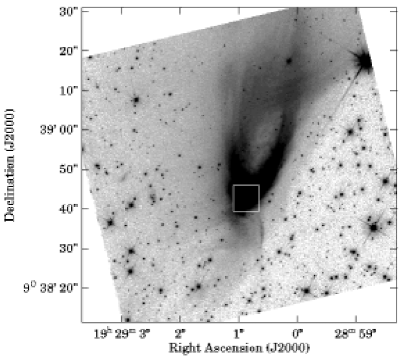
Figure 1: HST/WFPC2 image of Parsamian 21 taken through the F814W filter. The intensity scale is square root and brightness increases from light to dark. The white square marks the area shown in the upper left panel of Fig. 2.

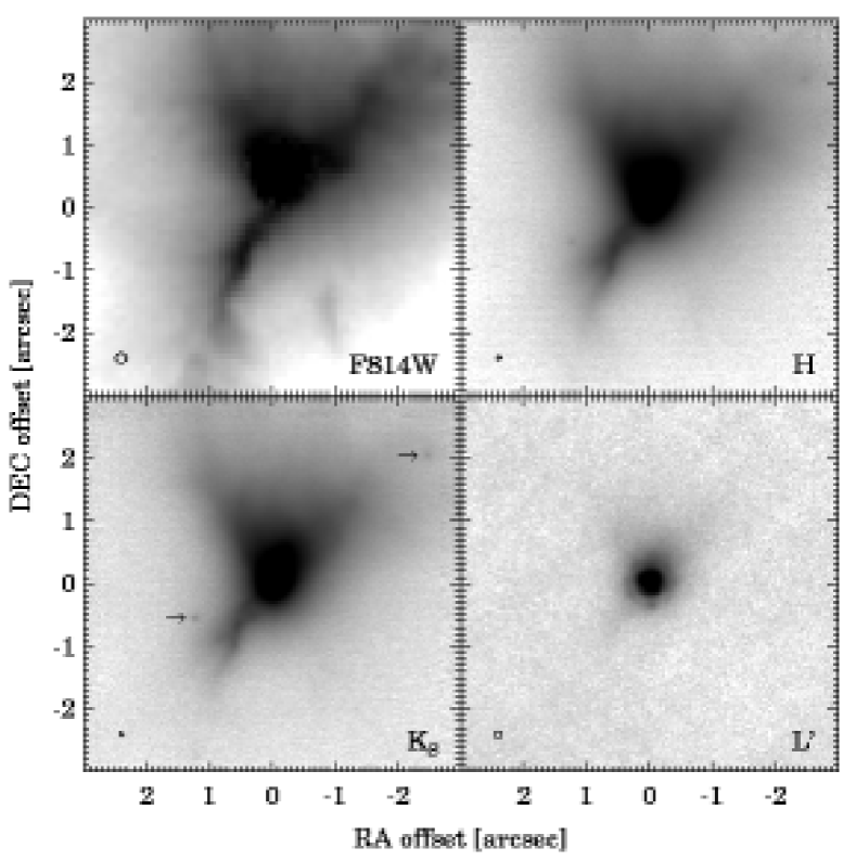
Figure 2: HST/WFPC2 (with filter F814W) and VLT/NACO (with filters H, K_S and L^′) images of Parsamian 21. Circles at the left bottom corners indicate the FWHM at the centre of the corresponding image. In the K_S-band image, arrows mark the positions of the two closest stars to Parsamian 21 (see Sect. 4.2).

Figure 1 displays the HST/WFPC2 image taken at $0.8\,\mu$m. The image reveals the structure of the Parsamian 21 nebula with an unprecedented spatial resolution and detail. We note that strong emission lines associated with the bipolar outflow (see Sect. 3.2) are not included in the bandpass, so the HST image provides a clean picture of the reflection nebula. The overall dimensions of the nebula are approximately $60\,{\times}\,20$ arcsec. The northern part has a characteristic elliptic, loop-like shape, with the inside of the loop having a relatively low surface brightness. The outer edge of the nebula is rather well-defined, while the inner edge is more fuzzy. Apart from the loop itself, there is also a wide, faint SE-NW oriented stripe about $30$ arcsec from the star. The nebula is clearly bipolar, although very asymmetric: the southern part is much less developed than the northern one. We note that while the southeastern arc is brighter close to the star (see the central part of the HST image in Fig. 2), the southwestern arc is more conspicuous farther from the star (Fig. 1). It is remarkable that field stars are visible both to the north and to the south of Parsamian 21. Supposing that these stars are in the background, this implies that there is no significant difference in the extinction between the northern and southern part.

Figure 2 shows the central parts of the HST/WFPC2 and the VLT/NACO images (note that the innermost $0.57$ arcsec of the HST image is saturated). The bipolar nature of the nebula is most conspicuous at the shortest wavelength ($0.8\,\mu$m), where all 4 arcs (roughly to the northeast, northwest, southwest and southeast) are visible. In the K_S and H bands the nebula is more triangle-shaped. In all three NACO bands the central source is extended, with deconvolved sizes of $0.20$, $0.12$ and $0.08$ arcsec in the H, K_S and L^′ bands, respectively.

3.2 Narrow-band imaging

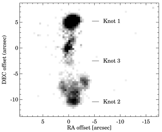
Figure 3: Continuum-subtracted H_α image of Parsamian 21. The peak at position (0,0) is the residuum of the central source. Three Herbig-Haro knots could be identified; these were named Knot 1, 2 and 3 by Staude & Neckel (1992).

Figure 4: South-north oriented cut across Parsamian 21 in the continuum-subtracted H_α image. 0 marks the position of the central star. The peaks marked by solid vertical lines at $-10.5$, $-3$ and $5$ arcsec correspond to Knot 2, 3 and 1, respectively. Dashed vertical lines mark the positions of the same knots as measured by Staude & Neckel (1992). Arrows demonstrate the direction where the knots propagate.

Figure 3 displays the continuum-subtracted H_α image of Parsamian 21. Conspicuous Herbig-Haro knots are seen to the north and the south of the central star. The northern knot is compact, resembling the knot described in Staude & Neckel (1992). The southern knot, however, has a distinctly bowed shape. The southern extent of this knot has a S/N of 10 over background per pixel, while the flanking structures have S/N $\approx$ 7. The northern knot has S/N in excess of 15 per pixel. To measure the angular distance of the knots from the central star in the H_α imagery, we binned the data in a 3 pixel (1.1 arcsec) wide swath oriented north-south. Apart from the residual of the central source, we could identify three knots (see Fig. 3): Knots 1, 2 and 3 are located 5 arcsec north, 10.5 arcsec south and 3 arcsec south, respectively. The knots correspond to those identified by Staude & Neckel (1992), but all three knots have moved outwards since then (Fig. 4). Assuming a distance of $400\,$pc, and supposing that the projected velocities are close to the velocities of the knots along the polar axis, one can derive $120\,$km s^-1 for Knots 1 and 3, and $530\,$km s^-1 for Knot 2. This is in good agreement with the velocities calculated by Staude & Neckel (1992) using radial velocity measurements. Such outflow velocities imply kinematic ages of approximately $80\,$yr for Knot 1 and $40\,$yr for Knots 2 and 3.

3.3 Spectral energy distribution

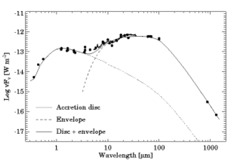
Figure 5: Complete UV-to-mm SED of Parsamian 21. Source of data: 2MASS All-Sky Catalog of Point Sources, MSX6C Infrared Point Source Catalog, Ábrahám et al. (2004), Polomski et al. (2005), Neckel & Staude (1984), Henning et al. (1998) and this work. The model SED is discussed in Sect. 4.4.

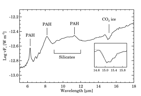
Figure 6: $5\,{-}\,18\,\mu$m part of the Spitzer/IRS spectrum of Parsamian 21. The inset displays in details the continuum-subtracted spectral region around the $15.2\,\mu$m CO₂ ice feature of Parsamian 21 with solid line and as a comparison HH 46 IRS with dashed line (for discussion see Sect. 4.5).

Table 2 contains our Spitzer and ISO photometry for Parsamian 21. These data, complemented with previously published measurements between 1983 and 1999 are plotted in Fig. 5, showing the complete UV-to-mm spectral energy distribution (SED) of the object. Comparing data taken between 1983 and 1999, Ábrahám et al. (2004) found that there is no long-term flux variation in the $1-100\,\mu$m wavelength range. The new Spitzer data from 2004 reveal that the mid-infrared brightness of Parsamian 21 stayed constant since then at a $15\%$ level. Although Parsamian et al. (1996) reported $2-3$ mag brightness variations in the B band between 1966 and 1990 (in Fig. 5 we plotted optical measurements from 1980 as representative values), no significant flux changes can be seen at longer wavelengths within the measurement uncertainties.

At wavelengths shorter than $3\,\mu$m, the SED is highly reddened (Polomski et al., 2005), probably due to the combined effect of interstellar extinction and self-shadowing by circumstellar material. The fact that the central source is extended at these wavelengths (see Sect. 3.1) indicates that the photometry is contaminated by scattered light from the inner part of the circumstellar environment. Between $3$ and $25\,\mu$m, the SED is rising towards longer wavelengths as $\nu F_{\nu}\,{\propto}\,\lambda$. The $5\,{-}\,18\,\mu$m Spitzer spectrum (Fig. 6) displays strong PAH emission features at $6.3$, $8.2$ and $11.3\,\mu$m and amorphous silicate emission around $10\,\mu$m (Quanz et al. 2007, see also the spectrum of Polomski et al. 2005). Weaker absorption features can also be seen between $7$ and $8\,\mu$m, which cannot be safely identified with any ice or PAH feature. The $10\,{-}\,19\,\mu$m channel of the Spitzer/IRS spectrum was not shown by Quanz et al. (2007) due to data reduction difficulties. We made an attempt to evaluate also this channel (for details, see Appendix). As can be seen in the inset of Fig. 6, the spectrum shows a strong CO₂ ice absorption feature at $15.2\,\mu$m, which has not been reported in the literature so far. Between $25$ and $100\,\mu$m the SED is flat ($\nu F_{\nu}\,{\propto}\,$const.), while the submillimetre shape is $\nu F_{\nu}\,{\propto}\,\lambda^{-3.5}$ (corresponding to $\beta\,{=}\,0.5$, assuming optically thin emission and a dust opacity law of $\kappa_{\nu}\,{\propto}\,\nu^{\beta}$). Using a distance of 400 pc and an interstellar reddening of $A_{V}\,{=}\,2\,$mag (Hillenbrand et al., 1992), the bolometric luminosity computed as the integral of the SED from $0.44$ to $1300\,\mu$m is $10\,$L_⊙ (assuming isotropic radiation field).

3.4 Polarimetry

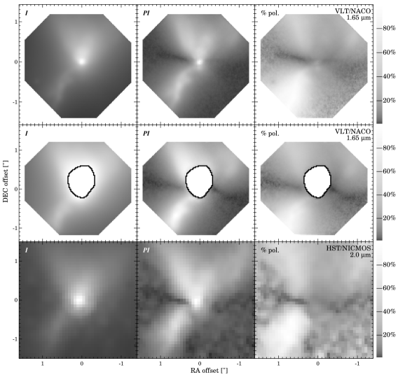
Figure 7: Left: total intensity ($I$); middle: polarized intensity ($PI$); right: degree of polarization (% pol.), with scalebar. Upper row: short exposure H-band NACO images; middle row: long exposure H-band NACO images (the saturated central parts are masked out); lower row: $2\,\mu$m NICMOS images of the same area. The intensity scale is logarithmic and brightness increases from dark to light.

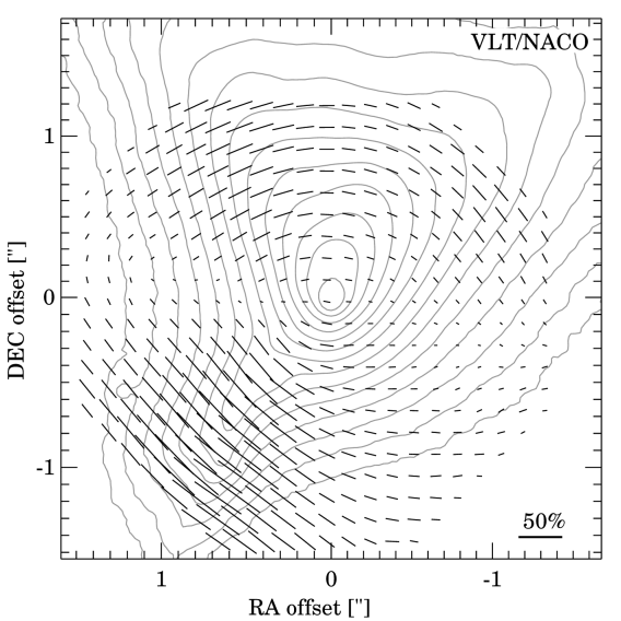
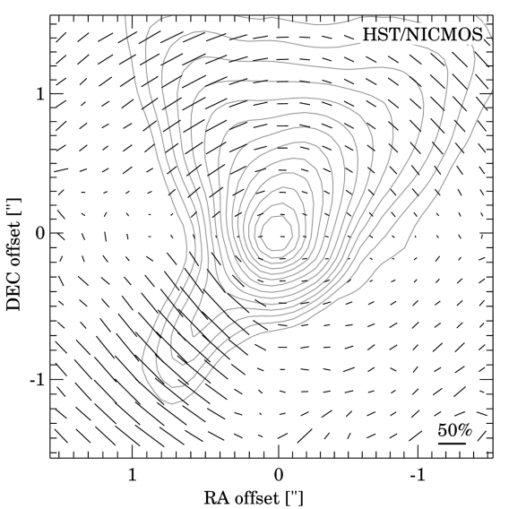
Figure 8: Polarization pseudovectors overlaid on intensity contours. Top: VLT/NACO, H-band, with $5\,{\times}\,5$ pixels binning, bottom: HST/NICMOS, $2\,\mu$m, with $2\,{\times}\,2$ pixels binning.

Figure 7 shows images of Parsamian 21 calculated from the H-band NACO polarization data, as well as from the $2\,\mu$m NICMOS measurements. The left column shows the total intensity ($I$) obtained as the sum of the intensities of the two orthogonal polarization states. The middle column displays the polarized intensity ($PI$) calculated as the square root of the quadratic sum of the $Q$ and $U$ Stokes components. The right column shows the degree of polarization (% pol.), i.e. the ratio of the polarized to the total intensity.

The NACO total intensity maps (Fig. 7, left) are very similar to the H-band map in Fig. 2. Thus, the Wollaston-prism data can reproduce well the direct images taken without the prism. While the total intensity is relatively smooth, the polarized intensity (Fig. 7, middle) reveals many fine details not visible in the total intensity map. The most striking feature is a dark horizontal lane across the star, where the polarized intensity is very low. Above this dark lane, high intensity regions can be seen, primarily emphasizing the walls of the upper lobe. Below the dark lane, the southeastern arc is very pronounced. The degree of polarization (Fig. 7, right) again shows features different from the previous two maps. Here, the central star almost disappears, as the stellar light is not polarized. The horizontal dark lane of low polarization across the star is even more pronounced: there the degree of polarization is around ${\approx}\,5\%$ in the H-band NACO images. We note that the polarization pattern in this area is probably affected by instrumental polarization (Sec. 2.1), though this effect should not alter our discussion in Sec. 4.3.2. The polarization of the central source itself, measured in a $0.08$ arcsec radius aperture, is $9\%$ and its position angle is $70^{\circ}$ east of north. The long exposure NACO images (Fig. 7, middle row), showing the outer regions with higher signal-to-noise ratio, are consistent with the short exposure maps (Fig. 7, upper row). It is remarkable that the NICMOS images, which represent independent observations (different resolution, different instrument, different polarization technique), show strikingly similar features, although the degree of polarization is slightly higher.

Figure 8 shows the polarization pseudovectors overlaid on total intensity contours. The NACO map, along with the degree of polarization map in Fig. 7 right shows that the horizontal band of low polarization across the star is very well-confined, narrow (about $0.15-0.20$ arcsec wide at the $5\%$ polarization level) and can be discerned from $0.12$ to $1.2$ arcsec to the star (and likely beyond, as indicated by the long exposure maps, see also the polarization maps of Draper et al. 1985 and Hajjar et al. 1997). The position angle of this band is $78^{\circ}\,{\pm}\,4^{\circ}$ east of north, consistent with that measured by Draper et al. (1985) ($75^{\circ}\,{\pm}\,4^{\circ}$). This implies that the band in our high spatial resolution images are a direct inward continuation of the band seen by Draper et al. (1985) and Hajjar et al. (1997) in their lower resolution images. The degree of polarization in this band is a few percent, and it is oriented parallel with the band itself.

Most of the northern part of the nebula shows a centrosymmetric pattern, characteristic of reflection nebulae with single scattering. This is consistent with what Draper et al. (1985) and Hajjar et al. (1997) measured for Parsamian 21 itself. It is also similar to what can be seen in other bipolar nebulae (see e.g. Meakin et al. 2005 for nebulae of young stars or Scarrott et al. 1993 for nebulae of evolved stars). The highest polarization in the northern part can be measured in the northeastern wall ($25-30\%$) and also in a spot about $0.9$ arcsec west and $0.6$ arcsec north to the star ($20-25\%$). The southern part of the nebula also follows the regular centrosymmetric pattern seen in the northern part. Here the highest polarization can be found in the southeastern arc ($60-70\%$).

The NICMOS vector map at $2\,\mu$m (Fig. 8 bottom) repeats all the main features seen by NACO in the H-band (Fig. 8 top). We note nevertheless the presence of two small, localized depolarization areas on either side of the central source at positions ($0\aas@@fstack{\prime\prime}9$, $0\aas@@fstack{\prime\prime}0$) and ($-0\aas@@fstack{\prime\prime}8$, $-0\aas@@fstack{\prime\prime}1$).

4 Discussion

4.1 Parsamian 21: an FU Orionis-type star

Although no optical outburst was ever observed, Parsamian 21 shares many properties characteristic of FUors. Its spectral type in the literature ranges from A5 to F8 supergiant (e.g.  Staude & Neckel, 1992), similar to the typical FUor spectral types (F–G supergiant). In addition, it shows strong infrared excess and drives a bipolar outflow, similarly to many FUors. However, in a recent paper by Quanz et al. (2007) the pre-main sequence nature and the FUor status of Parsamian 21 were questioned, mainly because its PAH emission bands are untypical for young stars. They suggest that Parsamian 21 is either an intermediate mass FUor object, or an evolved star sharing typical properties with post-AGB stars.

An important parameter which may discriminate between a pre-main sequence object and a post-AGB star is the luminosity. The typical luminosity of post-AGB stars is in the order of $10^{3}-10^{4}\,$L_⊙ (Kwok, 1993), while FUors are typically fainter than a few $100\,$L_⊙. The luminosity of Parsamian 21, $10\,$L_⊙ (see Sect. 3.3), is at least a factor of 100 lower than that of post-AGB stars. Even adopting the largest distance estimate mentioned in the literature (1800 pc, Staude & Neckel 1992), the luminosity of Parsamian 21 is still too low. The observed proper motion of the Herbig-Haro knots, however, prefers the lower distance (400 pc), otherwise the outflow velocities (${\approx}\,2400\,$km s^-1 at 1800 pc) would be unusually high for a young stellar object (typically up to $600\,$km s^-1, see e.g.  Mundt et al., 1987; Hessman et al., 1991). Moreover, the existence of Herbig-Haro outflows are usually tracers of low-mass star formation (Reipurth & Bally, 2001).

In the following discussion, we consider Parsamian 21 to be a FUor and we discuss its properties in the context of young eruptive stars. Nevertheless we note that most of our results on the morphology and circumstellar structure are valid regardless of the nature of the central object.

4.2 Parsamian 21: an isolated young star?

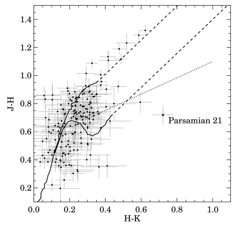
Figure 9: 2MASS colour-colour diagram of 188 sources in an area of $5.3\,{\times}\,5.3$ arcmin centred on Parsamian 21. The main-sequence and giant branch are marked by solid lines (Koornneef, 1983), the reddening path with dashed lines (Cardelli et al., 1989) and the T Tauri locus with dotted line (Meyer et al., 1997).

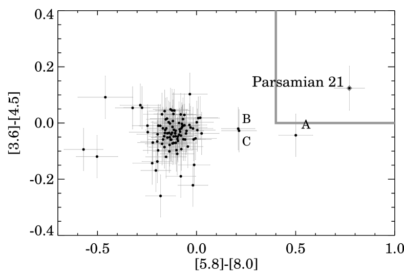
Figure 10: IRAC colour-colour diagram of 100 sources located in the same area as in Fig. 9. The gray square in the upper right corner marks the approximate domain of Class II sources (Allen et al., 2004).

Table 3: VLT/NACO photometry for the two closest stars. Uncertainties are about 0.1 mag.

$\alpha_{2000}$	$\delta_{2000}$	H mag	KS mag	L′ mag
19h 29m 0$\aas@@fstack{s}$96	9° 38′ 42$\aas@@fstack{\prime\prime}$11	20.2	19.1	$>$14.6
19h 29m 0$\aas@@fstack{s}$70	9° 38′ 44$\aas@@fstack{\prime\prime}$78	20.6	19.5	$>$14.4

Parsamian 21 is situated close to the Galactic plane ($l=45.8^{\circ}$, $b=-3.8^{\circ}$), in a molecular cloud called Cloud A. This cloud was identified by Dame & Thaddeus (1985) in their CO survey of molecular clouds in the northern Milky Way. The cloud occupies an area of 8 square degrees in the sky, and the only known young star associated with it is the T Tauri star AS 353 (Dame & Thaddeus, 1985).

In order to check whether FUors are usually associated with star forming regions, we searched the literature and found that most FUors are located in areas of active star formation (e.g. Henning et al., 1998). To find out whether there is star formation in the vicinity of Parsamian 21, we searched for pre-main sequence stars. For this purpose we constructed a 2MASS J$-$H vs. H$-$K_S and an IRAC [3.6]$-$[4.5] vs. [5.8]$-$[8.0] colour-colour diagram for sources found in our $5\aas@@fstack{\prime}3\,{\times}\,5\aas@@fstack{\prime}3$ IRAC field of view (Fig. 9, 10). Our selection criteria in the case of 2MASS was S/N ${>}\,10$ and uncertainties ${<}\,0.1\,$mag in all J, H and K_S bands, while in the case of IRAC S/N ${>}\,3$ and detectability at all four bands were required. The 2MASS diagram revealed that most of the nearby objects are reddened main sequence or giant stars. On the IRAC diagram, however, there are three objects (apart from Parsamian 21 itself), which display infrared excess at $8\,\mu$m (marked by A, B and C in Fig. 10). According to the classification of Allen et al. (2004), Class II sources exhibit colours of [3.6]$-$[4.5] ${>}\,0.0$ and [5.8]$-$[8.0] ${>}\,0.4$, thus one of these stars (A) might be a Class II source, while B and C are more likely Class III/main sequence sources. The nature of source A and its possible relationship to Parsamian 21 is yet to be investigated. Nevertheless, Parsamian 21 seems to be rather isolated compared to most FUors and certainly not associated with any rich cluster of young stellar objects.

We also searched for possible close companions of Parsamian 21 in the WFPC2 and NACO direct images. In order to establish a detection limit for source detection, we measured the sky brightness on the NACO images (before sky-subtraction), and estimated a limiting magnitude for each filter. The resulting values are $22.8$, $21.6$, and $15.2\,$mag in H, K_S and L^′, respectively. In case of the HST/WFPC2 image, the larger ($80\,{\times}\,80$ arcsec) field of view made it possible to estimate a limiting magnitude using star counts; the resulting value is $23.5\,$mag. Due to the bright reflection nebula, the detection limit is somewhat lower close to the star. The two closest objects we found are the following: one star to the southeast, at a distance of $1.4$ arcsec (560 AU at 400 pc), and another one to the northwest, at a distance of $3.3$ arcsec (1320 AU at 400 pc). These sources are marked with arrows in Fig. 2. Neither of the stars are visible at $3.8$ or $0.814\,\mu$m, although we can give an upper limit for their L^′ brightness. Their positions and photometry are given in Table 3. As these sources are very red, they can equally be heavily reddened background stars, or stars with infrared excess (indicating that they might be associated with Parsamian 21). Supposing that they are reddened main sequence stars, one can estimate an extinction of A${}_{V}\,{\approx}\,10\,{-}\,15\,$mag. Further multifilter observations may help to clarify the nature of these objects and their possible relationship to Parsamian 21.

4.3 The circumstellar environment of Parsamian 21

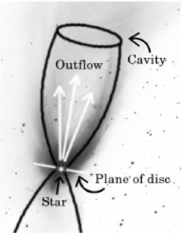
Figure 11: Sketch of the morphology of circumstellar material around Parsamian 21, overlaid on the HST/WFPC2 image. The central star is surrounded by an edge-on disc. Perpendicular to the disc, the star drives a bipolar outflow that excavates an outflow cavity in the dense circumstellar material. Light from the central star illuminates the walls of the cavity.

Figure 12: Brightness profiles of Parsamian 21 at $0.8\,\mu$m and in the H and K_S bands. Dotted lines mark Hubble’s relation.

Figure 13: South-north cut at $0.6$ arcsec east from the star. Solid line: total intensity; dashed line: polarized intensity.

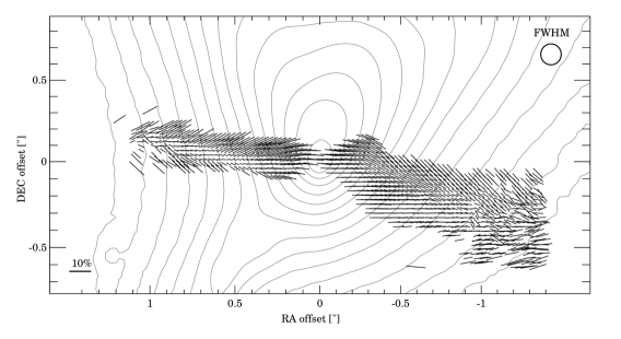
Figure 14: VLT/NACO polarization map of Parsamian 21 overlaid on H-band total intensity contours. The circle in the upper right corner displays the FWHM of the polarization measurement. Polarization vectors are displayed at full resolution, only showing the central low polarization band, where the polarization vectors are aligned. Such arrangement is expected when multiple scattering occurs in an edge-on disc.

The appearance and polarization properties of the nebula around Parsamian 21 can be understood in the following way: the star drives an approximately north-south oriented bipolar outflow, which had excavated a conical cavity in the dense circumstellar material (Fig. 11). The star illuminates this cavity and the light is scattered towards us mainly from the walls of the cavity. The outflow direction is perpendicular to an almost edge-on dense circumstellar disc. This picture is supported by the following facts: (a) the centrosymmetric polarization pattern is characteristic of reflection nebulae with single scattering; (b) the morphology and limb brightening suggest a hollow cavity (as opposed to an “outflow nebula”, where the lobes are composed of dense material ejected by the central source); and (c) the low-polarization lane across the star strongly suggests the presence of an edge-on circumstellar disc, where multiple scattering occurs. In general the Parsamian 21 system shows similarities to the NGC 2261 nebula associated with R Mon. This object also consists of a northern cometary nebula and a southern jetlike feature (Warren-Smith et al., 1987).

4.3.1 Envelope/Cavity

We characterised the opening of the upper lobe by marking the ridge along the northeastern and northwestern arcs which we interpret as the walls of the cavity. As viewed from the star northwards, the cavity starts as a cone with an opening angle of ${\approx}\,60^{\circ}$, giving the nebula in Fig. 2 a characteristic equilateral triangle-shape. Farther away from the star the cavity deviates from the conical shape, becomes narrower. The whole cavity occupies an area of $8\,000\,{\times}\,24\,000\,$AU (at a distance of $400\,$pc). The sharp outer boundary of the nebula implies a significant density contrast between the cavity and the surrounding envelope.

In Fig. 12 we plotted radial brightness profiles at $0.8\,\mu$m and in the H and K_S bands, starting from the star northwards. The slope of the intensity profiles in the inner ${\sim}\,1.6^{\prime\prime}$ ($640\,$AU) follows closely Hubble’s relation (Hubble, 1922), i.e. the brightness is proportional to r^-2. This trend can be clearly followed above the noise out to about $5\,$arcsec in our H and K_S images, giving an estimate of $2000\,$AU for the outer size of the envelope. The fact that the brightness profiles follow Hubble’s relation implies that the nebula is produced by isotropic single scattering, in accordance with the centrosymmetric polarization pattern and the high degree of polarization. Around ${\sim}\,1.6^{\prime\prime}$ the profiles becomes steeper, probably due to decreased density in the inside of the cavity. Similar steepening in the outer part of the nebula was already mentioned by Li et al. (1994). The profiles are similar at all observed wavelengths and do not show significant dependence on the position angle.

4.3.2 Disc

As mentioned in Sect. 3.4, both the NACO and NICMOS polarimetric images show a lane of low polarization oriented nearly east-west across the star (Fig. 7). The drop in the degree of polarization can also be clearly seen in Fig. 13, where a north-south cut at $0\aas@@fstack{\prime\prime}6$ east to the star is plotted. Following Bastien & Ménard (1990), we interpret the low polarization by multiple scattering in an edge-on disc (possible other explanations for the origin of the low polarization areas are discussed in e.g. Lucas & Roche 1998). According to models of such circumstellar structures (e.g. Whitney & Hartmann, 1993; Fischer et al., 1996) the polarization vectors are oriented parallel to the disc plane. As can be seen in Fig. 14, despite the low degree of polarization, the predicted alignment of the vectors can be clearly seen in the case of Parsamian 21 too. The NICMOS polarization map shows a similar effect. The dark lane in Fig. 7 can be followed inwards to as close as $48\,$AU from the star. This is an upper limit for the inner radius of the circumstellar disc.

An interesting feature of the mentioned models is two depolarized areas on either side of the central star, which mark the outer end points of an edge-on disc. The depolarization is due to a transition from the linearly aligned to the centro-symmetic polarization pattern. These depolarized areas can be seen in Fig. 8 bottom, on both sides at about $0.9^{\prime\prime}$ from the star. At the distance of Parsamian 21 this corresponds to $360\,$AU, and can be adopted as the outer radius of the dense part of the disc, where multiple scattering at near-infrared wavelengths is dominant. It is interesting that the NACO map does not show clear depolarized areas at the same position, but seems to resolve the transition in vector orientation, while the larger beam of NICMOS averaged the differently oriented vectors, resulting in depolarized spots.

The polarized intensity and degree of polarization images in Fig. 7 suggest a slight asymmetry in the dense disc: the eastern (left) side is straight, while the western (right) side shows a kink and also has a different position angle than that on the other side. The thickness of the disc can be measured on the area where the polarization vectors are aligned (Fig. 14). This approximately corresponds to the area where the degree of polarization is below ${\approx}\,10\%$. The resulting thickness is approximately $0.1^{\prime\prime}$ ($40\,$AU) to the east and is somewhat larger, $0.2^{\prime\prime}$ ($80\,$AU), to the west. One should note that, since these values are close to the spatial resolution of the polarimetric images, these numbers should be considered as upper limits for the thickness of the circumstellar disc around Parsamian 21. They are upper limits also because if the inclination is not exactly 90^∘, the thickness of the disc can be even less. The thickness does not show significant increase with radial distance, suggesting the picture of a flat, rather than a flared disc, at least considering the dense, multiple-scattering part. The smooth brightness and polarization distribution between the disc and the surrounding envelope (Fig. 13), however, implies that there is a continuous density transition between the two components. From the ratio of the horizontal to vertical sizes of the disc a lower limit of $84^{\circ}$ for the inclination of the system (the angle between the normal of the disc and the line of sight) can be derived.

Fischer et al. (1996) computed a grid of polarization maps of young stellar objects with the aim of helping the interpretation of polarimetric imaging observations. They consider five different models, four with massive, self-gravitating discs and one with a massless Keplerian disc. Since the mass of circumstellar material of Parsamian 21 derived from submillimetre observations is relatively low (${<}\,0.3\,$M_⊙, Henning et al. 1998; Polomski et al. 2005; Sandell & Weintraub 2001; Hillenbrand et al. 1992), the most appropriate model for our case is a Keplerian disc. Indeed the polarization pattern as computed by Fischer et al. (1996) for an inclination of 87^∘ (their Fig. 1) looks remarkably similar to our Fig. 8 (the differences might be explained by the narrower cavity and flatter disc of Parsamian 21). Thus, the geometry and structure assumed by Fischer et al. (1996) in their Keplerian model could be a good starting point for further radiative transfer modelling of Parsamian 21.

4.4 Modelling the circumstellar environment

Table 4: Model parameters. Parameters in italics are fixed, while the others were fitted.

Parameter	Variable	Value
Inner disc radius	$R_{1}$	3.5 $R_{\odot}$
Outer disc radius	$R_{2}$	360 AU
Temperature at 1 AU	$T_{\rm d,0}$	285 K
Power-law index for temperature	$q_{\rm d}$	0.75
Power-law index for surface density	$p_{\rm d}$	1.6
Disc mass	$M_{\rm d}$	0.02 M⊙
Inclination	$i$	86∘
Inner envelope radius	$R_{3}$	5.4 AU
Outer envelope radius	$R_{4}$	2000 AU
Temperature at 5 AU	$T_{\rm e,0}$	368 K
Power-law index for temperature	$q_{\rm e}$	0.4
Power-law index for surface density	$p_{\rm e}$	0.4
Envelope mass	$M_{\rm e}$	0.02 M⊙
Interstellar Extinction	$A_{V}$	2 mag

Our observations provide some direct measurements of the geometry of the circumstellar structure (disc size and thickness, inclination, envelope size). In the following we discuss the consistency of this picture with the observed SED. Our approach is to construct a simple disc+envelope model, in which we fix those parameters whose values are known from our NACO observations or from other sources (outer disc radius from this work; power-law index for disc temperature from Shakura & Sunyaev 1973; disc mass was set in order to ensure that the whole disc is optically thick; inclination from this work; outer envelope radius from this work, the power-law index for envelope temperature is a typical value for optically thin envelopes containing larger than interstellar grains, e.g. Hartmann 2000, Eqn. 4.13; interstellar extinction from Hillenbrand et al. 1992). Then we check whether the SED can be fitted by tuning the remaining parameters. We adopted an analytical disk model (Adams et al., 1987), which has been successfully used to model FUors (Quanz et al., 2006; Ábrahám et al., 2006). Our model consists of two components, an optically thick and geometrically thin accretion disc (Shakura & Sunyaev, 1973) and an optically thin envelope (no cavity is assumed). No central star is included in the simulation, partly because in outbursting FUors the star’s contribution is negligible compared to that of the inner disc (Hartmann & Kenyon, 1996), and partly because of the edge-on geometry where the star is obscured by the disc. This assumption is supported by the fact that the shape of the SED at optical wavelengths is broader than a stellar photosphere. The model also does not take into account internal extinction and light scattering, thus it cannot reproduce any of the near-IR imaging and polarimetric observations.

The temperature and surface density distribution in the disc are described by power-laws:

$$T(r)=T_{{\rm d},0}\left(\frac{r}{1\,{\rm AU}}\right)^{-q_{\rm d}},$$ (1)

$$\Sigma(r)=\Sigma_{{\rm d},0}\left(\frac{r}{1\,{\rm AU}}\right)^{-p_{\rm d}}.$$ (2)

Similar power-laws were assumed for the envelope. The observed flux at a specific frequency is given by

$$F_{\nu} = \frac{\cos{i}}{D^{2}}\int_{\rm R1}^{\rm R2}2\pi r(1-e^{\frac{-\Sigma_{{\rm d}}\kappa_{\nu}}{\cos{i}}})B_{\nu}(T_{\rm d}){\rm d}r+$$ (4)

$$\frac{1}{D^{2}}\int_{\rm R3}^{\rm R4}2\pi r(1-e^{-\Sigma_{{\rm e}}\kappa_{\nu}})B_{\nu}(T_{{\rm e}}){\rm d}r.$$

The first term describes the emission of the accretion disc, the second term describes the radiation of the optically thin envelope. For the dust opacity we used a constant value of $\kappa_{\nu}\,{=}$ 1 cm²g^-1 at $\lambda\,{>}\,1300\,\mu$m, $\kappa_{\nu}\,{=}\,\kappa_{1300\mu\rm m}\left(\frac{\lambda}{1300\mu\rm m}\right)^{-1}$ between $1300$ and $100\,\mu$m and again a constant value of $\kappa_{\nu}\,{=}\,\kappa(100\,\mu\rm m)$ at $\lambda\,{<}\,100\,\mu$m.

We fitted the SED via $\chi^{2}$ minimisation using a genetic optimization algorithm PIKAIA (Charbonneau, 1995). This algorithm performs the maximization of a user defined function, for which purpose we used the inverse $\chi^{2}$. Since there are many photometric measurements in the mid-infrared domain, but just a few in the far-infrared, the mid-infrared region has a higher weight during the fit, compared to the far-infrared domain. Therefore, in order to ensure an equally good fit at all wavelengths, we divided the SED into four regions and weighted the $\chi^{2}$ of each domain with the inverse of number of photmetric points the region contained. Then the final $\chi^{2}$ was the sum of the $\chi^{2}$ of all regions. The regions we used were: $0.3-3$, $3-30$, $30-300$ and $300-3000\,\mu$m. The parameters of the best-fit model, which gives a weighted $\chi^{2}$ of 0.67, are listed in Table 4. The fitted model SED as well as the disc and envelope components are overplotted in Fig. 5.

The model SED is consistent with the observed fluxes. This shows that the picture of a thin accretion disc and an envelope is consistent with both the measured SED and the geometry and disc/envelope parameters inferred from our polarimetric observations. Detailed modelling of the silicate, PAH, and ice spectral features, as well as the correct treatment of internal extinction and scattering would require radiative transfer modelling, which will be the topic of a subsequent paper.

4.5 The evolutionary status of Parsamian 21

The geometry of FUor models discussed in the literature (e.g. Hartmann & Kenyon 1996; Turner et al. 1997) usually consist of a central star surrounded by an accretion disc and an infalling envelope with a wind-driven polar hole. These assumptions are supported by the fact that they fit well the SED (Green et al., 2006; Quanz et al., 2007), the interferometric visibilities (Millan-Gabet et al., 2006b; Ábrahám et al., 2006) and the temporal evolution of the SED (Ábrahám et al., 2004). In this paper we present the first direct imaging of these circumstellar structures in a FUor. Our polarimetric measurements of Parsamian 21 show the existence of a circumstellar disc which extends from at least 48 to 360 AU. The most striking feature of the disc is its flatness over the whole observed range. The short-wavelength part of the SED could be well reproduced using a radial temperature profile of $r^{-0.75}$ (Sect. 4.4). This profile is expected from both a geometrically thin accretion disc and a flat reprocessing disc. An envelope was also seen in the polarization maps of Parsamian 21 and it was also a necessary component for the SED modelling. Envelopes are involved in many FUor models and in this paper we present a direct detection of this model component. Our images reveal that the envelope can be followed inwards as close to the star as the disc. FUor models often assume a polar cavity in the envelope, created by a strong outflow or disc wind. The direct images of Parsamian 21 clearly show the presence of such a cavity and we also detected a bipolar outflow in the Parsamian 21 system.

In the recent years, as new interferometric and infrared spectroscopic observations were published for FUors, the group turned out to be more inhomogeneous in physical properties than earlier assumed, when mainly optical photometry and spectroscopy had been available. Quanz et al. (2007) proposed that some differences might be understood as an evolutionary sequence. They suggest that FUors constitute the link between embedded Class I objects and the more evolved Class II objects. Members of the group exhibiting silicate absorption at $10\,\mu$m are younger and more embedded (Category 1, e.g. V346 Nor); while objects with pure silicate emission are more evolved (Category 2, e.g. FU Ori and Bran 76). There are objects showing a superposition of silicate absorption and emission, which are probably in an intermediary evolutionary stage (e.g. RNO 1B). Green et al. (2006) also sorted FUors, based on the ratio of the far-infrared excess and the luminosity of the central accretion disc, $f_{d}$ (Equ. 7 in their paper). A large relative excess ($f_{d}\,{>}\,5\%$) indicates an envelope of large covering fraction (V1057 Cyg and V1515 Cyg), while low relative excess means a tenuous or completely missing envelope (Bran 76 and FU Ori). This is also an evolutionary sequence, as young, more embedded objects have large envelopes, while around more evolved stars, the envelope has already dispersed. $f_{d}$ can also be used to calculate the opening angle of the envelope, thus a prediction of this scheme is that the opening angle is becoming wider during the evolution, probably due to strong outflows during the repeated FUor outbursts.

The two classification schemes are not inconsistent and one can merge them into the following evolutionary sequence: (1) the youngest objects exhibit silicate absorption and large far-infrared excess (V346 Nor, probably also OO Ser and L1551 IRS 5 belong here); (2) intermediate-aged objects, where the silicate feature is already in emission but there is still a significant far-infrared excess (V1057 Cyg, V1515 Cyg, probably also RNO 1B and V1647 Ori); (3) the most evolved objects show pure silicate emission and low far-infrared excess (FU Ori, Bran 76). We note, however, that this classification has some weak points. As Quanz et al. (2007) already mentioned, an edge-on geometry in a more evolved system may appear as a younger one. Moreover, during an outburst and the subsequent fading phase, certain spectral features as well as the global shape of the SED may change.

Parsamian 21 can be placed in this evolutionary scheme, though one should keep in mind that because of the nearly edge-on geometry, the classification of this object is somewhat uncertain. Parsamian 21 displays silicate emission (Fig. 6). Integrating the flux of the two components in our simple model (Sect. 4.4), and correcting the apparent disc luminosity for inclination effect ($i=86^{\circ}$, Table 4) using Equ. 6 of Green et al. (2006), we obtained a large relative far infrared excess of $f_{d}\,{=}\,75\%$. These two properties place Parsamian 21 into the intermediate-aged category (though because of its inclination, it may actually seem younger than it is). Following Equ. 7 of Green et al. (2006), from the $f_{d}$ value, we also computed the opening angle of the envelope. The resulting opening angle of $60^{\circ}$ agrees well with the angle measured in the direct NACO images (Sect. 4.3.1).

Parsamian 21 was placed into the evolutionary scheme using two parameters: the silicate feature and the relative far infrared excess. In the following we discuss whether its other physical characteristics match with those of other FUors.

• Our observations revealed that the circumstellar disc of Parsamian 21 is very flat. Due to lack of similar direct measurements for other FUors, we can only speculate that perhaps all FUors with envelopes have such flat discs. On the other hand, the most evolved FUor, FU Ori, seems to have no envelope but its disc is probably flared (Kenyon & Hartmann, 1991; Green et al., 2006; Quanz et al., 2006). This might suggest that disc flaring develops at later stages, when illumination from the central source may heat the disc surface more directly.

• In a nearly edge-on system like Parsamian 21, one expects to see the $10\,\mu$m silicate feature in absorption. The fact that Parsamian 21 has silicate emission indicates that the line of sight towards the central region is not completely obscured. Using the optical depth of the $15.2\,\mu$m CO₂ ice feature, we calculated an $A_{V}\,{=}\,8\,$mag ($A_{V}\,{=}\,38.7A_{15.2\mu\rm{}m}$, Savage & Mathis 1979). This value is surprisingly low compared to V1057 Cyg ($A_{V}\,{\sim}\,50-100\,$mag, Kenyon & Hartmann 1991). This indicates a much more tenuous envelope, which is also supported by the low envelope mass of $0.02\,\rm{}M_{\odot}$ in our modelling.

• Following Quanz et al. (2007), we analysed the profile of the $15.2\,\mu$m CO₂ ice feature of Parsamian 21. The inset in Fig. 6 shows that the feature has a characteristic double-peaked sub-structure, very similar to HH 46 IRS, an embedded young source (Boogert et al., 2004). HH 46 IRS is a reference case for processed ice. The presence of processed ice in Parsamian 21 indicates heating processes and the segregation of CO₂ and H₂O ice, already at this evolutionary stage. Other FUors exhibiting this kind of profile are L1551 IRS 5, RNO 1B and RNO 1C (Quanz et al., 2007).

The evolutionary state of a young stellar object can also be estimated following the method proposed by Chen et al. (1995). According to their Equ. (1) we calculated a bolometric temperature of T${}_{\rm bol}=410\,$K for the measured SED. We compared this value with the distribution of corresponding values among young stellar objects in the Taurus and $\rho\,$Ophiuchus star forming regions (Chen et al. 1995). From this check we can conclude that Parsamian 21 seems to be a class I object, and its age is ${\sim}\,10^{5}\,$yr. However, Green et al. (2006) argued that the apparent SED of the disc component depends on the inclination. Thus we computed T_bol also for a face-on disc configuration and obtained T${}_{\rm bol}=1160\,$K, corresponding to a Class II object. In fact, Parsamian 21 is probably close to the Class I / Class II border, in accordance with the proposal of Quanz et al. (2007).

5 Summary

We present the first high spatial resolution near-infrared direct and polarimetric observations of Parsamian 21, with the VLT/NACO instrument. We complemented these measurements with archival infrared observations, such as HST/WFPC2 imaging, HST/NICMOS polarimetry, Spitzer IRAC and MIPS photometry, Spitzer IRS spectroscopy as well as ISO photometry. Our main conclusions are the following:

• We argue that Parsamian 21 is probably an FU Orionis-type object;

• Parsamian 21 is not associated with any known rich cluster of young stars;

• our measurements reveal a circumstellar envelope, a polar cavity and an edge-on disc; the disc seems to be geometrically flat and extends from at least 48 to 360 AU from the star;

• the SED is consistent with a simple circumstellar disc + envelope model;

• within the framework of an evolutionary sequence of FUors proposed by Quanz et al. (2007) and Green et al. (2006), Parsamian 21 can be classified as an intermediate-aged object.

Appendix A Refined calibration of the Spitzer/IRS beam profiles

Table 5: Log of IRS calibration measurements.

Channel	AOR	Date	Target
Short Low	16295168	2005-Nov-21	HR 7341
	19324160	2006-Jul-5	HR 7341
Short High	16294912	2005-Nov-21	HR 6688
Long Low	16463104	2005-Dec-19	HR 6606
Long High	16101888	2005-Oct-18	HR 2491

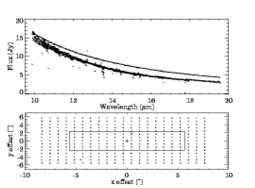
Figure 15: Top: Dots show the measured spectrum of HR 6688, obtained with Spitzer/IRS through the Short High slit; the continuous line show a model spectrum of the same star (from Decin et al., 2004). Bottom: Scheme of the data grid; the $+$ sign marks the slit centre; dots show the position of the star relative to the slit centre; the rectangle indicates the slit itself; the $\times$ sign marks the position where the spectrum plotted in the top panel was taken.

Figure 16: Beam profiles of the four Spitzer/IRS channels, perpendicular to the slit, at selected wavelengths. Filled dots show the measured profile, while open dots indicate the pixelized model PSF.

In those cases when the source is not well centred in the slit, part of the stellar PSF falls outside of the slit, leading to flux loss. When the precise absolute flux level of the spectrum is important, one should correct for this flux loss. Correction for this kind of flux loss is not implemented in the Spitzer data reduction pipeline. For point sources flux loss in off-centred sources can be efficiently corrected if we know the beam profiles of the different IRS slits. In order to construct the beam profiles for all four IRS slits, we reduced and analysed dedicated IRS calibration measurements taken in spectral mapping mode in a regular grid. Table 5 shows a log of these calibration measurements. We used the pipeline processed post-BCD files (pipeline version S14.0.0). At each spatial position, we divided the measured spectrum with a synthetic MARCS model spectrum appropriate for the measured star (Decin et al., 2004). The result is a data cube with two spatial dimensions and one wavelength dimension. We resampled these data cubes to finer spatial grid and smoothed them in wavelength.

We checked whether the measured beam profiles are consistent with the PSFs provided by Spitzer’s Tiny Tim (J. Krist). In Fig. 16 we plotted the ratio between the observed and the model spectrum at different distances from the slit centre at a certain wavelength. We found slight differences: the measured profiles were in general narrower than the model PSFs, and in some cases they were not centred at zero. We examined several effects that can cause a difference between the model and the measured profiles and we found that the differences can be attributed to pixelization effects (pixel sizes are $1.8^{\prime\prime}$ for SL, $2.3^{\prime\prime}$ for SH, $5.1^{\prime\prime}$ for LL and $4.5^{\prime\prime}$ for LH) and to small (few tenths of arcsecond) uncertainties in the exact position of the calibration star with respect to the slit. Based on our analysis, we decided to use the measured profiles to correct our science measurements, and to use the TinyTim model profiles to estimate the uncertainty of the correction. Using this correction, the absolute flux level of IRS spectra has an uncertainty of 10%, but individual measurements can be much more precise if the source is well-centred in the slit and the necessary correction is small. More details on IRS beam profiles will be given in a future paper.

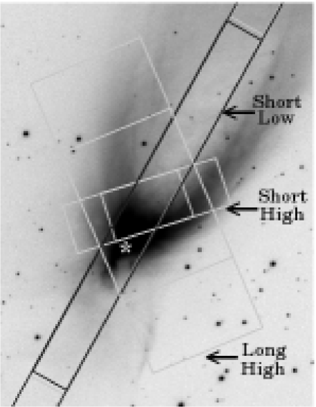
Figure 17: Positions of the Spitzer/IRS slits with respect to Parsamian 21 (marked with an asterisk). Black rectangle: Short Low, small grey rectangle: Short High, big grey rectangle: Long High.

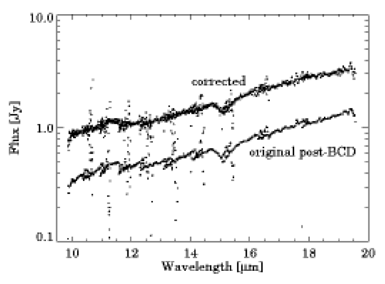
Figure 18: Short High channel spectrum of Parsamian 21.

Figure 17 shows the position of the IRS slits overplotted on the HST/WFPC2 image of Parsamian 21. While the target is well-centred in the Short Low slit, it is slightly off-centred in the Long High and it is practically off-slit in the Short High. Considering our measured beam profiles, we found that no correction is necessary in the Short Low channel, a small correction ($5-20\%$, depending on wavelength) is necessary in the Long High channel, and a significant correction must be made in the Short High channel, where the corrected flux is approximately 3-4 times the original one (see Fig. 18). After the correction, the different IRS channels match fairly well in the overlapping wavelength regimes.

References

- Ábrahám et al. (2004) Ábrahám P., Kóspál Á., Csizmadia S., et al., 2004, A&A, 428, 89
- Ábrahám et al. (2006) Ábrahám P., Mosoni L., Henning T., et al., 2006, A&A, 449, L13
- Adams et al. (1987) Adams F. C., Lada C. J., Shu F. H., 1987, ApJ, 312, 788
- Allen et al. (2004) Allen L. E., Calvet N., D’Alessio P., et al., 2004, ApJS, 154, 363
- Apai et al. (2004) Apai D., Pascucci I., Brandner W., et al., 2004, A&A, 415, 671
- Bastien & Ménard (1990) Bastien P., Ménard F., 1990, ApJ, 364, 232
- Boley et al. (2006) Boley A. C., Mejía A. C., Durisen R. H., et al., 2006, ApJ, 651, 517
- Boogert et al. (2004) Boogert A. C. A., Pontoppidan K. M., Lahuis F., et al., 2004, ApJSS, 154, 359
- Bouchet et al. (1991) Bouchet P., Schmider F. X., Manfroid J., 1991, Ap&SS, 91, 409
- Cardelli et al. (1989) Cardelli J. A., Clayton G. C., Mathis J. S., 1989, ApJ, 345, 245
- Charbonneau (1995) Charbonneau 1995, ApJS, 101, 309
- Chen et al. (1995) Chen H., Myers P. C., Ladd E. F., et al., 1995, ApJ, 445, 377
- Dame & Thaddeus (1985) Dame T., Thaddeus P., 1985, ApJ, 297, 751
- Decin et al. (2004) Decin L., Morris P., Appleton P. N., Charmandaris V., Armus L., Houck J. R., 2004, ApJS, 154, 408
- Diolaiti et al. (2000) Diolaiti E., Bendinelli O., Bonaccini D., et al., 2000, Proc. SPIE, 4007, 879
- Draper et al. (1985) Draper P. W., Warren-Smith R. F., Scarrott S. M., 1985, MNRAS, 212, 1P
- Fischer et al. (1996) Fischer O., Henning T., Yorke H. W., 1996, A&A, 308, 863
- Green et al. (2006) Green J. D., Hartmann L., Calvet N., et al., 2006, ApJ, 648, 1099
- Hajjar et al. (1997) Hajjar R., Bastien P., Nadeau D., 1997, Canada-France-Hawaii Telescope Information Bulletin, 37, 3
- Hartmann (2000) Hartmann L., 2000, Accretion Processes in Star Formation. Cambridge University Press
- Hartmann & Kenyon (1996) Hartmann L., Kenyon S. J., 1996, ARA&A, 34, 207
- Hartung et al. (2000) Hartung M., Bizenberger P., Boehm A., et al., 2000, in Proc. SPIE Vol. 4008, p. 830-841, Optical and IR Telescope Instrumentation and Detectors, Masanori Iye; Alan F. Moorwood; Eds. First test results and calibration methods of CONICA as a stand-alone device. pp 830–841
- Henning et al. (1998) Henning T., Burkert A., Launhardt R., et al., 1998, A&A, 336, 565
- Herbig (1977) Herbig G. H., 1977, ApJ, 217, 693
- Herbig et al. (2003) Herbig G. H., Petrov P. P., Duemmler R., 2003, ApJ, 595, 384
- Hessman et al. (1991) Hessman F. V., Eisloeffel J., Mundt R., et al., 1991, ApJ, 370, 384
- Hillenbrand et al. (1992) Hillenbrand L. A., Strom S. E., Vrba F. J., et al., 1992, ApJ, 397, 613
- Hines et al. (2000) Hines D. C., Schmidt G. D., Schneider G., 2000, PASP, 112, 983
- Hines & Schneider (2006) Hines D. C., Schneider G., 2006, in Proceedings of the 2005 HST calibration workshop Polarimetry with nicmos. p. 153
- Hubble (1922) Hubble E. P., 1922, ApJ, 56, 400
- Kenyon & Hartmann (1991) Kenyon S. J., Hartmann L. W., 1991, ApJ, 383, 664
- Koornneef (1983) Koornneef J., 1983, A&A, 128, 84
- Kuhn et al. (2001) Kuhn J. R., Potter D., Parise B., 2001, ApJ, 553, L189
- Kwok (1993) Kwok S., 1993, ARA&A, 31, 63
- Lenzen et al. (1998) Lenzen R., Hofmann R., Bizenberger P., et al., 1998, in Proc. SPIE Vol. 3354, p. 606-614, Infrared Astronomical Instrumentation, Albert M. Fowler; Ed. CONICA: the high-resolution near-infrared camera for the ESO VLT. pp 606–614
- Li et al. (1994) Li W., Evans N., Harvey P., et al., 1994, ApJ, 433, 199
- Lucas & Roche (1998) Lucas P. W., Roche P. F., 1998, MNRAS, 299, 69
- Malbet et al. (1998) Malbet F., Berger J.-P., Colavita M. M., et al., 1998, ApJ, 507, L149
- Malbet et al. (2005) Malbet F., Lachaume R., Berger J.-P., et al., 2005, A&A, 437, 627
- Mazzuca & Hines (1999) Mazzuca L., Hines D., 1999, Instruemnt Science Report NICMOS ISR-99-004
- Meakin et al. (2005) Meakin C. A., Hines D. C., Thompson R. I., 2005, ApJ, 634, 1146
- Meyer et al. (1997) Meyer M. R., Calvet N., Hillenbrand L. A., 1997, AJ, 114, 288
- Millan-Gabet et al. (2006a) Millan-Gabet R., Monnier J. D., Akeson R. L., et al., 2006a, ApJ, 641, 547
- Millan-Gabet et al. (2006b) Millan-Gabet R., Monnier J. D., Akeson R. L., et al., 2006b, ApJ, 641, 547
- Mundt et al. (1987) Mundt R., Brugel E. W., Buehrke T., 1987, ApJ, 319, 275
- Neckel & Staude (1984) Neckel T., Staude H. J., 1984, A&A, 131, 200
- Parsamian (1965) Parsamian E., 1965, Izv. Akad. Nauk Armyan. SSR., Ser., 18, 146
- Parsamian et al. (1996) Parsamian E. S., Gasparian K. G., Ohanian G. B., 1996, Astrophysics, 39, 121
- Persson et al. (1998) Persson S. E., Murphy D. C., Krzeminski W., et al., 1998, AJ, 116, 2475
- Polomski et al. (2005) Polomski E. F., Woodward C. E., Holmes E. K., et al., 2005, AJ, 129, 1035
- Quanz et al. (2007) Quanz S., Henning T., Bouwman J., et al., 2007, ApJ, in press, ApJ preprint doi: 10.1086/’521219’
- Quanz et al. (2006) Quanz S. P., Henning T., Bouwman J., et al., 2006, ApJ, 648, 472
- Reipurth & Bally (2001) Reipurth B., Bally J., 2001, ARA&A, 39, 403
- Rousset et al. (2003) Rousset G., Lacombe F., Puget P., et al., 2003, in Adaptive Optical System Technologies II. Edited by Wizinowich, Peter L.; Bonaccini, Domenico. Proceedings of the SPIE, Volume 4839, pp. 140-149 (2003). NAOS, the first AO system of the VLT: on-sky performance. pp 140–149
- Sandell & Weintraub (2001) Sandell G., Weintraub D. A., 2001, ApJ, 134, 115
- Savage & Mathis (1979) Savage Mathis 1979, ARA&A, 17, 73
- Scarrott et al. (1993) Scarrott R. M. J., Scarrott S. M., Wolstencroft R. D., 1993, MNRAS, 264, 740
- Shakura & Sunyaev (1973) Shakura N. I., Sunyaev R. A., 1973, A&A, 24, 337
- Staude & Neckel (1992) Staude H. J., Neckel T., 1992, ApJ, 400, 556
- Tuffs & Gabriel (2003) Tuffs R. J., Gabriel C., 2003, A&A, 410, 1075
- Turner et al. (1997) Turner N. J. J., Bodenheimer P., Bell K. R., 1997, ApJ, 480, 754
- Vorobyov & Basu (2006) Vorobyov E. I., Basu S., 2006, ApJ, 650, 956
- Warren-Smith et al. (1987) Warren-Smith R. F., Draper P. W., Scarrott S. M., 1987, ApJ, 315, 500
- Wassell et al. (2006) Wassell E., Grady C.A.and Woodgate B., et al., 2006, ApJ, 650, 985
- Whitney & Hartmann (1993) Whitney B. A., Hartmann L., 1993, ApJ, 402, 605
- Whittet et al. (1992) Whittet D. C. B., Martin P. G., Hough J. H., et al., 1992, ApJ, 386, 562