Biconical structures in two–dimensional anisotropic Heisenberg antiferromagnets

Abstract

Square lattice Heisenberg and XY antiferromagnets with uniaxial anisotropy in a field along the easy axis are studied. Based on ground state considerations and Monte Carlo simulations, the role of biconical structures in the transition region between the antiferromagnetic and spin–flop phases is analyzed. In particular, adding a single–ion anisotropy to the XXZ antiferromagnet, one observes, depending on the sign of that anisotropy, either an intervening biconical phase or a direct transition of first order separating the two phases. In case of the anisotropic XY model, the degeneracy of the ground state, at a critical field, in antiferromagnetic, spin–flop, and bidirectional structures seems to result, as in the case of the XXZ model, in a narrow disordered phase between the antiferromagnetic and spin–flop phases, dominated by bidirectional fluctuations.

Recently, two–dimensional uniaxially anisotropic Heisenberg antiferromagnets in a magnetic field along the easy axis have been studied theoretically rather intensively Mat ; Leidl1 ; Holt1 ; Zhou1 ; Leidl2 ; Holt2 ; Vic ; Schwing ; Zhou2 , motivated by experiments on intriguing magnetic properties of layered cuprates Mat ; Ammer ; Pokro ; Rev1 ; Rev2 and by experimental findings on complex phase diagrams for other quasi two–dimensional antiferromagnets Bevaart ; Gaulin ; Cowley ; Chris ; Pini exhibiting, typically, multicritical behavior.

A generic model describing such systems is the XXZ Heisenberg antiferromagnet on a square lattice, with the Hamiltonian

$${\cal H}=J\sum\limits_{(i,j)}\left[\Delta(S_{i}^{x}S_{j}^{x}+S_{i}^{y}S_{j}^{y})+S_{i}^{z}S_{j}^{z}\right]-H\sum\limits_{i}S_{i}^{z}$$ (1)

where we consider the classical variant, with the spin at site $i$, $\vec{S}_{i}=[S_{i}^{x},S_{i}^{y},S_{i}^{z}]$, being a vector of length one. $\vec{S}_{i}$ is coupled to its four neighboring spins $\vec{S}_{j}$ at sites $j$. The exchange integral $J$ is antiferromagnetic, $J>0$, and the anisotropy parameter $\Delta$ may vary from zero (Ising limit) to one (isotropic Heisenberg model). The magnetic field $H$ acts along the easy axis, the $z$–axis. As known for many years LanBin , the phase diagram of the XXZ model includes the long–range ordered antiferromagnetic (AF), the algebraically ordered spin–flop (SF), and the paramagnetic phases. Only very recently, attention has been drawn to the role of biconical (BC) structures and fluctuations, in the ground state and in the transition region between the AF and SF phases Holt2 .

In a BC ground state configuration the spins on the two sublattices (i.e. on neighboring sites), $A$ and $B$, form different cones around their two different tilt angles, $\theta_{A}$ and $\theta_{B}$, with respect to the easy axis, see Fig. 1. In the XXZ model, these structures occur at the critical field, $H_{c1}$, which separates the AF and SF structures at $T=0$. The two tilt angles of the BC ground states are interrelated by Holt2 .

$$\theta_{B}=\arccos\left(\frac{\sqrt{1-\Delta^{2}}\;-\;\cos\theta_{A}}{1\;-\;\sqrt{1-\Delta^{2}}\cos\theta_{A}}\right)$$ (2)

leading, in addition to the rotational symmetry in the xy-components of the spins in the BC and SF states, to a high degeneracy of the ground state. This degeneracy seems to give rise to a narrow intervening, possibly disordered phase in the (field $H$, temperature $T$)–phase diagram of the square lattice XXZ model, as discussed before Holt2 ; Holt1 ; Zhou1 .

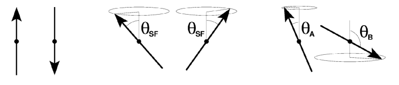
Figure 1: Spin orientations on neighboring sites in the ground states of the XXZ models (without and with additional single–ion anisotropy), corresponding to, from left to right, antiferromagnetic, spin–flop, and biconical configurations.

In this communication, we study variants of the XXZ model, staying in two dimensions, by adding a single–ion anisotropy, and by reducing the XXZ to the anisotropic XY model. Results will be based on ground state calculations and Monte Carlo simulations. The aim is to analyze the effect of these modifications on the biconical (or their ’bidirectional’ analogues for the XY variant) structures and fluctuations, both for the ground states and for the phase diagrams.

Biconical structures can be stabilized in various ways, starting with the XXZ model, especially by taking into account further anisotropies, for instance, a cubic anisotropy, or couplings to spins at more distant sites Tsun ; Fisher ; Bruce . Here, a single–ion anisotropy will be added, reflecting crystal symmetry. Similar properties are expected for related anisotropies as well. The single–ion anisotropy term has the form

$${\cal H}_{si}=D\sum\limits_{i}(S_{i}^{z})^{2}$$ (3)

which either, $D<0$, enhances the uniaxial anisotropy $\Delta$, or, $D>0$, may weaken it due to a competing planar anisotropy. The sign of $D$ will have drastic consequences for the phase diagram. In both cases, the ground state properties can be determined exactly Holt3 .

In case of a positive single–ion anisotropy, $D>0$, BC structures are ground states in a non–zero range of fields, $H_{c1a}<H<H_{c1b}$, in between the AF ($H\leq H_{c1a}$) and SF ($H\geq H_{c1b}$) structures Holt3 . Note that at fixed field in that range, only BC structures with a unique pair of tilt angles $\theta_{A}$ and $\theta_{B}$, are stable, with a modified relation between the angles, compared to Eq. (2), depending now also on $D$. At $T>0$, there is a BC phase, ordered simultaneously in the spin components parallel and perpendicular to the easy axis Fisher , intervening between the AF and SF phases. This is found in extensive Monte Carlo simulations studying square lattices with up to $L\times L=240\times 240$ sites, and performing runs with up to $10^{8}$ Monte Carlo steps per site (MCS), applying the standard Metropolis algorithm. A typical phase diagram is shown in Fig. 2, where we set $\Delta=0.8$, as usual LanBin ; Holt1 ; Zhou1 , and $D/J=0.2$. The phase boundaries are determined by finite–size extrapolations of the staggered susceptibilities, the specific heat, and the Binder cumulant Holt3 . Obviously, see Fig. 2, the extent of the BC phase shrinks with increasing temperature. Eventually, the BC phase may terminate at a tetracritical point Fisher ; Bruce ; Muka ; Hu ; Aharony ; Cala , where the AF, SF, BC and paramagnetic phases meet. It may be estimated to be roughly at $k_{B}T/J=0.35\pm 0.05$.

Figure 2: Simulated phase diagram of the XXZ model, $\Delta=0.8$, with an additional positive single–ion anisotropy, $D=0.2$. The squares denote the SF, the circles the AF phase boundary. Error bars are omitted unless they are larger than the symbol sizes.

The critical properties of the boundary lines of the BC phase to the AF and SF phases have been simulated and studied in much detail at $k_{B}T/J=0.2$, see Fig. 2. The boundary line between the BC and SF phases, where the staggered magnetization in the direction of the field (or ’longitudinal staggered magnetization’) vanishes, seems to belong to the Ising universality class. For example, the effective critical exponent of that susceptibility is found to approach 7/4, when analyzing the size dependence of the peak height Holt3 . Note that, in this case, large systems, $L\geq 120$, are needed for getting close to the supposed asymptotics. In turn, at the boundary line between the BC and AF phases the algebraic order in the transverse staggered magnetization, which we observe in the BC phase, gets lost. The finite-size behavior of that magnetization, for $L\geq 40$, agrees with the transition belonging to the Kosterlitz–Thouless universality class. Note that renormalization group arguments on the universality classes of the boundary lines of biconical phases Bruce suggest transitions in the Ising and XY–universality classes as well.

In case of a negative single-ion anisotropy, $D<0$, at all fields, no BC structures are ground states. At low temperatures, the Monte Carlo simulations (with computational efforts as for $D>0$) provide evidence for a direct transition of first order between the AF and SF phases. Such evidence is exemplified in Fig. 3 for $\Delta=0.8$ and $D/J=-0.2$, where the peak height of the longitudinal staggered susceptibility, $\chi_{max}$, is shown to grow with size $L$ proportionally to $L^{2}$, as expected for a transition of first order. The coexistence of the AF and SF phases at a first–order transition is also seen in the behavior of the probability $P(\theta)$ to find the tilt angle $\theta$ in a configuration. $P(\theta)$ shows more and more pronounced maxima at the values of $\theta$ characterizing the AF and SF phases, when increasing the system size. Note that for small system sizes, biconical fluctuations are observed in the transition region between the AF and SF phases Holt3 .

Figure 3: Selected raw data for the longitudinal staggered susceptibility $\chi_{st}^{z}$ versus field at fixed temperature, $k_{B}T/J=0.3$ near the transition, $H_{AF}/J=2.798\pm 0.0005$, between the AF and SF phases for the XXZ model, $\Delta=0.8$, $D=-0.2$. Data for Systems of sizes 20 (circles), 40 (squares), and 80 (diamonds) are shown. In the inset, the finite–size, $L$, dependence of the peak height, $\chi_{max}$, is depicted, with the straight, solid line showing $\chi_{max}\propto L^{2}$. Error bars are included when they are larger than the symbol sizes.

Let us turn to another variant of the XXZ model, the anisotropic XY antiferromagnet. According to renormalization group calculations Koster ; Cala ; Vic , applied to the case of uniaxiality, the number of spin components $n$ is expected to determine the nature of the multicritical point, at which the AF, SF, and, possibly, BC phases meet with the paramagnetic phase. For $n$ being not too large, the multicritical point has been supposed to be a bicritical, tetracritical or critical end–point. Now, in two dimensions, a bicritical point of O(n)–symmetry with $n=3$, as it is the case in the XXZ model, is ruled out at a non-zero temperature in two dimensions by the well–known Mermin–Wagner theorem. However, it may occur when reducing the number of spin components from $n=3$ to $n=2$. Then the bicritical point would be of O(2)–symmetry, and thus would be allowed at $T>0$, belonging to the Kosterlitz–Thouless universality class. Thence, it looks interesting to consider the $n=2$ variant of the XXZ antiferromagnet, namely the anisotropic XY model, described by the Hamiltonian

$${\cal H}=J\sum\limits_{(i,j)}\left[(S_{i}^{x}S_{j}^{x}+\Delta S_{i}^{y}S_{j}^{y})\right]-H\sum\limits_{i}S_{i}^{x}$$ (4)

with the classical spins having now only two components.

The ground state analysis can be done in complete analogy to the one for the XXZ model. Of course, the spins are now restricted to the XY–plane, and the tilt angle $\theta$ is defined for the spin orientation with respect to the easy $x$–axis. Especially, the biconical structures are replaced by bidirectional (BD) structures. At the critical field, $H_{c1}$, the AF and SF structures are degenerate with the set of BD configurations, for which $\theta_{A}$ and $\theta_{B}$ are interrelated as in the XXZ case, Eq. (2).

Figure 4: Simulated phase diagram of the anisotropic XY model, with $\Delta=0.8$. The squares denote the phase boundary of the SF, the circles the one of the AF phase. The inset magnifies the part, where AF and SF phase boundaries approach each other.

The phase diagram of the anisotropic XY antiferromagnet, with $\Delta$= 0.8, is depicted in Fig. 4. It has been obtained from extensive Monte Carlo simulations studying lattices sizes up to $L\times L=120\times 120$, and performing runs with up to $10^{8}$ MCS. The phase boundaries are determined by finite–size extrapolations, similar to the analysis for the XXZ model with a single–ion anisotropy.

The topology of the phase diagram looks like in the XXZ case LanBin ; Holt1 ; Zhou1 . The AF and SF boundary lines approach each other very closely near the maximum of the SF phase boundary in the $(T,H)$–plane, see Fig. 4. Accordingly, at low temperatures, there seems to be either a direct transition between the AF and SF phases, or two separate transitions with an extremely narrow intervening phase may occur.

Away from that intriguing transition region, one expects the transition not only from the AF but also the one from the SF phase to the paramagnetic phase to be in the Ising universality class. In the SF phase of the XY antiferromagnet, there is just one ordering component, the $y$–component. The expectation is confirmed by the Monte Carlo data for the specific heat (where the peak at the AF phase boundary gets rather weak on approach to the transition region) and for the staggered susceptibilities. The quantities exhibit critical behavior of Ising–type, as follows from the corresponding effective exponents describing size dependences of the various peak heights.

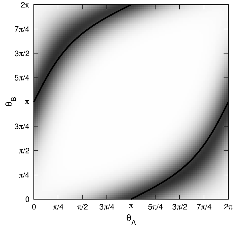
Figure 5: Joint probability $p(\theta_{A},\theta_{B})$ for the anisotropic XY antiferromagnet with $\Delta$= 0.8 for a system with $100\times 100$ lattice sites in the transition region between the AF and SF phases at $k_{B}T/J=0.558$ and $H/J=2.44$. $p(\theta_{A},\theta_{B})$ is proportional to the grayscale. The superimposed solid line depicts the relation between the two tilt angles in the ground state, see Eq. (2).

In the transition region of the AF and SF phases, BD fluctuations dominate, as one may conveniently infer from the joint probability distribution $p(\theta_{A},\theta_{B})$ for finding the tilt angles $\theta_{A}$ and $\theta_{B}$ at neighboring sites, i.e. for the two different sublattices. A typical result is depicted in Fig. 5, showing the behavior of $p$ in a grayscale representation. Two features are of interest: first, the two tilt angles are strongly correlated like in the degenerate ground state, with a line of local maxima in $p$ closely following Eq. (2). Second, all those bidirectional structures occur simultaneously with (almost) equal probability, i.e. along the line of maxima $p$ is (almost) constant. Note that this behavior is only weakly affected by finite–size effects for the system sizes we simulated. Moving away from the transition region, for instance, by fixing the temperature and varying the field, the line of local maxima initially does not change significantly, but, along that line, pronounced peaks start to show up at positions corresponding to the AF, at lower fields, or to the SF phases, at higher fields. Similar observations for the joint probability distribution hold for the XXZ model without single–ion anisotropy Holt2 .

Additional evidence on critical phenomena in the transition region may be obtained by analyzing effective exponents. We did that for the staggered susceptibilities and the specific heat. Results (especially, at $H/J=2.44$ and $0.54<k_{B}T/J<0.57$) are compatible with Ising–type criticality, but rather large corrections to scaling had to be presumed. For example, the effective critical exponents for describing the size–dependences of the peak height for the staggered susceptibilities are about 1.8 to 1.85, largely independent of system size. The supposedly strong corrections to scaling may be due to very large correlation lengths in that region, and the asymptotics may be reached only for very large systems.

To conclude, the simulational data seem to suggest for the anisotropic XY antiferromagnet the existence of an extremely narrow, presumably, disordered phase, intervening between the AF and SF phases, like in the XXZ case Holt1 ; Zhou1 . The transition region between the two phases is clearly dominated by, in the ground state completely degenerate, bidirectional fluctuations.

- (1) M. Matsuda, K. Kakurai, J. E. Lorenzo, L. P. Regnault, A. Hiess, and G. Shirane, Phys. Rev. B 68, 060406(R) (2003).
- (2) R. Leidl and W. Selke, Phys. Rev. B 70, 174425 (2004).
- (3) M. Holtschneider, W. Selke, and R. Leidl, Phys. Rev. B 72, 064443 (2005).
- (4) C. Zhou, D. P. Landau, and T. C. Schulthess, Phys. Rev. B 74, 064407 (2006).
- (5) R. Leidl, R. Klingeler, B. Büchner, M. Holtschneider, and W. Selke, Phys. Rev. B 73, 224415 (2006).
- (6) M. Holtschneider, S. Wessel, and W. Selke, Phys. Rev. B 75, 224417 (2007).
- (7) A. Pelissetto and E. Vicari, Phys. Rev. B 76, 024436 (2007).
- (8) U. Schwingenschlögl and C. Schuster, Europhys. Lett. 79, 27003 (2007).
- (9) C. Zhou, D. P. Landau, and T. C. Schulthess, Phys. Rev. B 76, 024433 (2007).
- (10) U. Ammerahl, B. Büchner, C. Kerpen, R. Gross, and A. Revcolevschi, Phys. Rev. B 62, R3592 (2000).
- (11) W. Selke, V. L. Pokrovsky, B. Büchner, and T. Kroll, Eur. Phys. J. B 30, 83 (2002).
- (12) T. Vuletić, B. Korin-Hamzić, T. Ivek, S. Tomić, B. Gorshunov, M. Dressel, and J. Akimitsu, Phys. Rep. 428, 169 (2006).
- (13) M. Uehara, N. Motoyama, M. Matsuda, H. Eisaki, and J. Akimitsu, in: A. V. Narlikar (Ed.), Frontiers in Magnetic Materials, Springer (2005).
- (14) L. Bevaart, E. Frikkee, and L. J. de Jongh, Phys. Rev. B 19, 4741 (1979).
- (15) B. D. Gaulin, T. E. Mason, M. F. Collins, and J. Z. Larese, Phys. Rev. Lett. 62, 1380 (1989).
- (16) R. A. Cowley, A. Aharony, R. J. Birgeneau, R. A. Pelcovits, G. Shirane, and T. R. Thurston, Z. Phys. B 93, 5 (1993).
- (17) R. J. Christianson, R. L. Leheny, R. J. Birgeneau, and R. W. Erwin, Phys. Rev. B 63, 140401(R) (2001).
- (18) M. G. Pini, A. Rettori, P. Betti, J. S. Jiang, Y. Ji, S. G. E. te Velthuis, G. P. Felcher, and S. D. Bader, J. Phys.: Condens. Matter 19, 136001 (2007).
- (19) K. Binder and D. P. Landau, Phys. Rev. B 13, 1140 (1976); D. P. Landau and K. Binder, Phys. Rev. B 24, 1391 (1981).
- (20) H. Matsuda and T. Tsuneto, Prog. Theoret. Phys. Suppl. 46, 411 (1970).
- (21) K.-S. Liu and M. E. Fisher, J. Low. Temp. Phys. 10, 655 (1973).
- (22) A. D. Bruce and A. Aharony, Phys. Rev. B 11, 478 (1975).
- (23) M. Holtschneider, PhD thesis, RWTH Aachen (2007).
- (24) D. Mukamel, Phys. Rev. B 14, 1303 (1976).
- (25) X. Hu, Phys. Rev. Lett. 87, 057004 (2001).
- (26) A. Aharony, J. Stat. Phys. 110, 659 (2003).
- (27) P. Calabrese, A. Pelissetto, and E. Vicari, Phys. Rev. B 67, 054505 (2003).
- (28) J. M. Kosterlitz, D. R. Nelson, and M. E. Fisher, Phys. Rev. B 13, 412 (1976).